Magnetic field production after inflation.

Abstract:

We study the electromagnetic field production during preheating after hybrid inflation in a model with the field content of the Standard Model, coupled to a singlet inflaton. We find that very soon after symmetry breaking our system enters a regime of kinetic turbulence, characterized by a self-similar behaviour of the energy spectra and a power-like dependence on time of the inflaton and Higgs field variances.

PoS(LAT2005)242

1 INTRODUCTION

There is a large amount of indirect observations of the presence of large scale cosmological magnetic fields (LSMF) with scales that go from the size of galaxies to the size of superclusters, with a relatively big strength [1]. It is believed that these magnetic fields were present in the form of a magnetic seed before the epoch of structure formation and that they were amplified to its present magnitude. Although there are several attempts to explain these magnetic field seeds, their origin is still a mystery [1]. It is tempting to speculate whether they could be generated within the inflationary paradigm [2]. Our present work is along these lines. Taking the end of inflation at the electroweak scale, we propose to place the origin of LSMF in the very out of equilibrium epoch called the preheating era. Our first aim is to throw some light into the process of electromagnetic field production during this period.

1.1 The model and the method

We consider a hybrid inflation model which has the field content of the Standard Model (SM) gauge-scalar sector plus a singlet scalar field, the inflaton, coupled to the SM Higgs:

$${\cal L}=-{1\over 4}G^{a}_{\mu\nu}G^{\mu\nu}_{a}-{1\over 4}F^{\rm Y}_{\mu\nu}F_{\rm Y}^{\mu\nu}+{\rm Tr}\Big{[}(D_{\mu}\Phi)^{\dagger}D^{\mu}\Phi\Big{]}+{1\over 2}(\partial_{\mu}\chi)^{2}-V(\Phi,\chi)\,,$$ (1)

with $\Phi={1\over 2}(\phi_{0}\,1\!{\rm l}+i\phi^{a}\tau_{a})$ the Higgs field, $\chi$ the inflaton and $G^{a}_{\mu\nu}=\partial_{\mu}A_{\nu}^{a}-\partial_{\nu}A_{\mu}^{a}+g_{{}_{\rm W}}\epsilon^{abc}A_{\mu}^{b}A_{\nu}^{c}$ and $F_{\mu\nu}^{\rm Y}=\partial_{\mu}B_{\nu}-\partial_{\nu}B_{\mu}$ the field strengths of the SU(2) and U(1) gauge fields respectively. The covariant derivative is: $D_{\mu}=\partial_{\mu}-{i\over 2}g_{{}_{\rm W}}A_{\mu}^{a}\tau_{a}-{i\over 2}g_{{}_{\rm Y}}B_{\mu}$, with $g_{{}_{\rm W}}$ the SU(2) gauge coupling and $g_{{}_{\rm Y}}$ the hypercharge U(1) coupling. The scalar potential includes a coupling to a massive inflaton:

$${\rm V}(\Phi,\chi)={\rm V}_{0}+{1\over 2}(g^{2}\chi^{2}-m^{2})\,|\phi|^{2}+\frac{\lambda}{4}|\phi|^{4}+{1\over 2}\mu^{2}\chi^{2}\,,$$ (2)

where $|\phi|^{2}\!\equiv\!2{\rm Tr}\,\Phi^{\dagger}\Phi$, $\mu$ is the inflaton mass in the false vacuum and $m\!\equiv\!\sqrt{\lambda}\,v$; $\,v\!=\!246$ GeV. During the period of hybrid inflation the inflaton field is dominated by its homogeneous mode $\chi_{0}$. Inflation ends at $t\!=\!t_{c}$ when this mode slow-rolls below $\chi_{c}\!\equiv\!m/g$ where the Higgs becomes massless. Around this time $\chi_{0}\!=\!\chi_{c}(1-Vm(t-t_{c}))$, with $V$ the inflaton dimensionless velocity. After $t_{c}$ a negative time-dependent mass-squared of the Higgs is induced. During the subsequent evolution, the low momentum modes of the Higgs grow exponentially in a process known as “tachyonic preheating” [3]. Preheating in this model has been proposed in Refs. [4, 5] as a mechanism for electroweak baryogenesis, an appealing possibility that has been numerically investigated in [4, 6, 7].

To compute the time evolution of the system after inflation ends, we have used the classical approximation (details can be found in [6] - see also [8]). For suitable parameter choices, the growth of the Higgs field low momentum modes takes place before non-linearities in the Higgs potential and the coupling to the gauge fields have become relevant. Thus, one can exactly compute the quantum evolution of the Higgs field. It is such that, after a while, the tachyonic modes of the Higgs evolve like classical modes. This initial stage is very fast and therefore the remaining degrees of freedom can be assumed to remain in their initial quantum vacuum (ground) state. Once sufficient number of Higgs modes have become classical we substitute the exact quantum evolution by the classical one. For consistency, this substitution should be done before non-linearities have become relevant. The advantage of this approximation is that it allows to treat the full non-linear evolution of the system by lattice techniques.

2 RESULTS

The results presented here correspond to the particular choice of parameters denoted as Model A1 in Ref. [6]. For this model the inflaton velocity $V\!=\!0.024$, $g^{2}\!=\!2\lambda$, $g_{{}_{\rm W}}\!=\!0.05$, and the Higgs to W boson mass ratio is given by $m_{{}_{\rm H}}/m_{{}_{\rm W}}\!=\!4.65$. Here we also introduce the U(1) hypercharge field, fixing $g_{{}_{\rm Y}}$ to reproduce the experimentally determined Weinberg angle. This choice of parameters, although far from the physical value of $m_{{}_{\rm W}}$, allows an optimal control of lattice and finite volume artefacts for the lattices sizes reachable with our present computer resources [6]. Results for physically relevant parameters will be presented elsewhere [9]. The chosen values of the lattice cut-off are $ma\!=\!1.31$ (NS=32), $ma\!=\!0.87$ (NS=48) and $ma\!=\!0.655$ (NS=64). The time-like lattice spacing $a_{t}$ must be smaller than the spatial one for the stability of the discretized equations of motion. We have chosen $a/a_{t}=40$ and $80$ and checked stability of the results under this change.

2.1 Means and Spectra

In Fig. 1 (Left), the time evolution of $\langle\overline{|\phi|}/v\rangle$ and $\langle\overline{\chi}/\chi_{c}\rangle$ illustrates the process of symmetry breaking: the Higgs starts in the false vacuum at $t=t_{c}$ and quickly evolves into the symmetry broken phase.

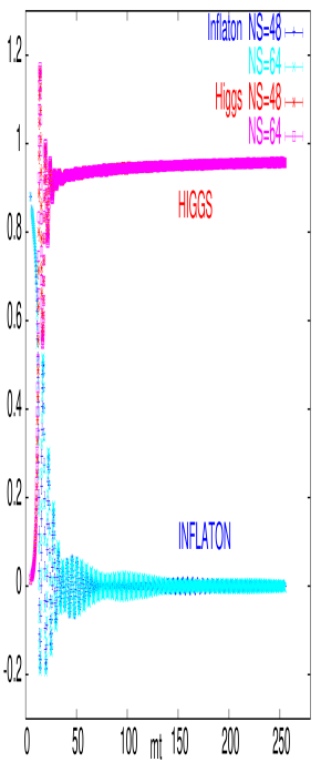
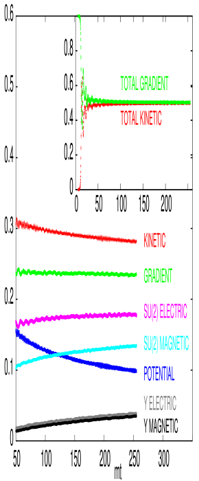
Figure 1: Left: The time evolution of $\langle\overline{|\phi|}/v\rangle$, $\langle\overline{\chi}/\chi_{c}\rangle$. Right: Late time behaviour of the different components of the energy, normalized to the total energy, for NS=48.

Fig. 1 (Right) shows the late time behaviour of the different components of the energy, normalized to the total energy, for $ma\!=\!0.87$. The evolution is such that kinetic and potential energies virialize as for harmonic oscillators ($\langle$kinetic$\rangle\!=\!\langle$potential$\rangle$).

We are interested in the behaviour of electromagnetic fields long after symmetry breaking. It is not obvious that our approximations remain under control for such late times. The validity of the classical approximation rests on the fact that the tachyonic infrared modes dominate the dynamics. This cannot happen if ultraviolet modes are strongly excited when the physically relevant processes take place. A way to expose the range of relevant momenta is to analyze the Fourier spectra of the (gauge invariant) energy densities. Fig. 2 shows, as an illustration, the time evolution of the spectra of the inflaton+Higgs contribution to the kinetic energy and of the electric component of the SU(2) gauge field energy. To enhance the effect of lattice artefacts for large momenta, we plot $k^{2}|E(k)|$. Note that the presence of the lattice cut-off truncates the range of allowed momenta. The number, $N(k)$, of lattice momenta of norm $k$ should be proportional to $k^{2}$ in the range of relevant momenta for the cut-off not to distort the physical spectrum. Deviations of $N(k)$ from the $k^{2}$ behaviour appear for $k/m>$ 2.5, 3.5, 4.5 for NS= 32, 48, 64 respectively. It is clear from the figure that the NS=32 lattice is off. NS=48 starts showing deviations, for physically relevant momenta, for times above $mt\!\sim\!100$. These deviations, however, seem to remain small up to much larger times. Full checks of cut-off independence by going to larger lattices will be done in the near future. Nevertheless, given these results, our approach to study the evolution up to relatively large times, $mt\!\sim\!250$, seems viable. The time ranges in this study are four times larger than those in Ref. [6].

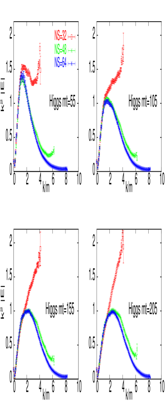
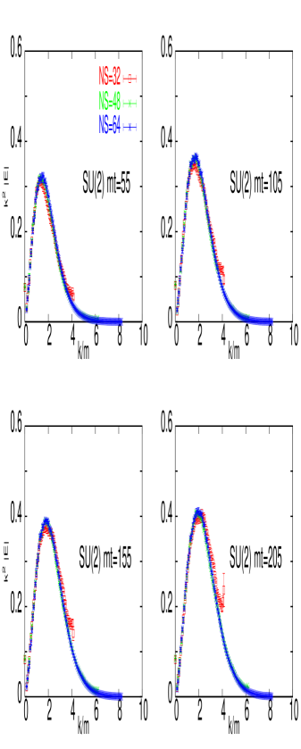
Figure 2: Spectra of the inflaton+Higgs kinetic energy and SU(2) electric energy.

2.2 Electromagnetic field production

In order to analyze the production of electromagnetic fields we have, first, to extract the U(1)_em content of the SU(2)$\times$U(1) fields in the Lagrangian. Details of the lattice implementation will be given elsewhere [9]. In terms of the SU(2) link, $U_{\mu}(x)$, and the hypercharge link, $\hat{B}_{\mu}(x)$, one can express the field associated to the $Z$ boson as:

$$\hat{Z}_{\mu}(n)=-{\rm Tr}\Big{(}i\tau_{3}\ {\Phi^{\dagger}(n)\over|\phi(n)|}\ U_{\mu}(n)\ {\Phi(n+\mu)\over|\phi(n+\mu)|}\ \hat{B}_{\mu}(n)\Big{)}\hskip 14.22636pt\stackrel{{\scriptstyle a\rightarrow 0}}{{\longrightarrow}}\hskip 14.22636pta_{\mu}g_{Z}Z_{\mu}\,,$$ (3)

with $a_{\mu\neq 0}=a$, $a_{0}=a_{t}$ and $g_{Z}$ the $Z$ boson coupling. The field strength of the U(1)_em field is obtained from: $\hat{F}^{{\rm em}}_{\mu\nu}(n)^{2}=1-\cos\Big{(}{g_{{}_{\rm Y}}^{2}\over g_{{}_{\rm Y}}^{2}+g_{{}_{\rm W}}^{2}}\hat{F}^{{\rm Z}}_{\mu\nu}(n)-\hat{F}^{{\rm Y}}_{\mu\nu}(n)\Big{)}\,,$ with $F^{\rm Z}_{\mu\nu}(n)\!=\!\hat{Z}_{\mu}(n)\!-\!\hat{Z}_{\nu}(n+\mu)\!-\!\hat{Z}_{\mu}(n+\nu)\!-\!\hat{Z}_{\nu}(n)$ and $\hat{F}^{\rm Y}_{\mu\nu}(n)\!=\!\hat{B}_{\mu}(n)\!-\!\hat{B}_{\nu}(n+\mu)\!-\!\hat{B}_{\mu}(n+\nu)\!-\!\hat{B}_{\nu}(n)$. In the continuum limit $\hat{F}^{{\rm em}}_{\mu\nu}\longrightarrow a_{\mu}a_{\nu}eF^{{\rm em}}_{\mu\nu}$, with $F^{{\rm em}}_{\mu\nu}$ the continuum electromagnetic field strength.

In computing the field strength of the $Z$ boson, $\hat{F}^{\rm Z}_{\mu\nu}$, from Eq. (3) there is a complication that arises due to the possible discontinuous behaviour of $\Phi^{\dagger}(n)/|\phi(n)|$ at points where the Higgs field is zero. At such points the $Z$ boson and the electromagnetic field strengths can show a (lattice) delta-function behaviour. This gives rise to the appearance of non-scaling spikes in the corresponding energy densities which affect also spatially averaged quantities. Although configuration averaging smears out the effect of the spikes, they give rise to a very noisy signal. One way to improve the signal is to eliminate from the spatial averages the points where the Higgs norm gets closer to zero than a certain value $|\phi_{c}|$. Taking $|\phi_{c}|=0.08$ considerably reduces the noise and gives results compatible within errors with those obtained from larger statistics sets. The appearance of these spikes is rather common in the first stages of the evolution where the Higgs field gets rather often close to zero. It becomes more rare as time evolves, although occasionally they can also occur at times at large as $mt=200$. It is attractive to speculate that these zeroes could be associated to sphaleron-like configurations, a point that deserves further investigation [9].

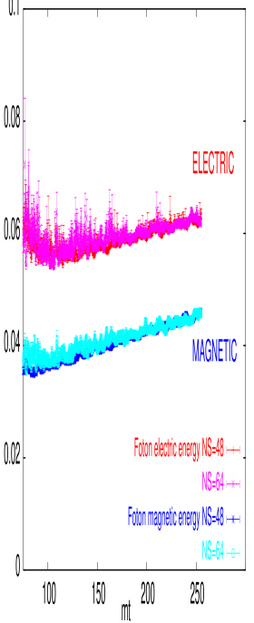
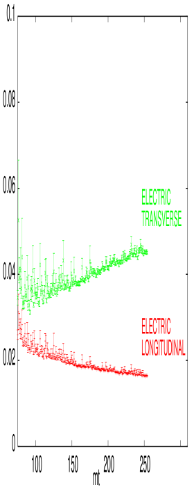
Figure 3: Left: Late time behaviour of the electric and magnetic components of the U(1)_em energy, normalized to the total energy. Right: Longitudinal and transverse parts of the electric component.

Figure 3 shows our final result for the late time behaviour of the electric and magnetic components of the U(1)_em energy, normalized to the total energy. Results are shown for two different lattice spacings, agreeing well within errors. A detailed analysis of the properties of the electromagnetic field will be deferred to a future paper [9]. Here we only want to point out that a separation between the longitudinal and transverse components of the electric field can be easily performed by going to Fourier space. The result is shown in Fig. 3 (Right). The longitudinal component decreases with time. This is the expected behaviour at large times since the system evolves into a plasma with charge density going to zero.

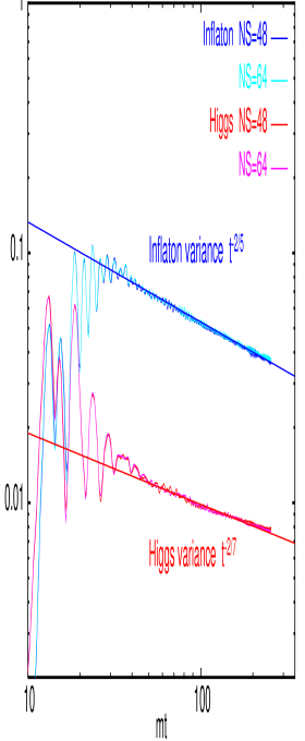
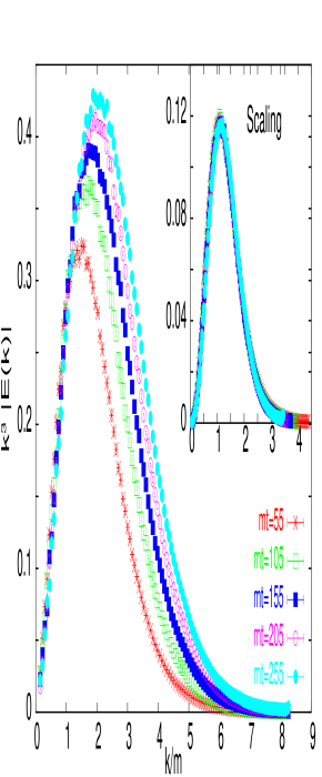
Figure 4: Left: The late time behaviour of the variance of the Higgs and inflaton fields. Right: Spectra of the SU(2) electric part of the energy showing a self-similar scaling according to Eq. (2.2).

2.3 Kinetic turbulence

According to Ref. [10], systems like the one we study evolve towards thermalization via a period of kinetic turbulence. This regime is characterized by a specific behaviour of the variance of the scalar fields together with a particular scaling of the energy spectra. To be concrete, one expects for the scalar fields: $\langle\phi^{2}\rangle-\langle\phi\rangle^{2}\sim t^{-\nu}$ with $\nu=2/(2m-1)$ in three spatial dimensions and for $m$-particle interactions. At the same time the energy spectra show a self-similar behaviour:

$$n(k,t)=t^{-q}n_{0}(kt^{-p}),\hskip 28.45274pt{\rm with}\hskip 14.22636ptn(k,t)\equiv{E(k,t)\over k}$$ (4)

where $q=3.5p$ and $p=1/(2m-1)$. Ref. [10] analyzes models containing only scalar fields. The characteristic times for the kinetic turbulence regime are $mt>3000$ after inflation ends. We also find that our data enter a regime of kinetic turbulence, but this happens at much earlier times $mt>50$, presumably due to the larger number of degrees of freedom. The variances of the Higgs and inflaton fields are shown in Fig. 4 (Left). They follow the expected behaviour with $m\!=\!4$ for the Higgs and $m\!=\!3$ for the inflaton. Fig. 4 (Right) shows the spectra of the electric part of the SU(2) energy for several times from $mt=55$ up to $mt=250$. The data remarkably follow the self-similar behaviour of Eq. (4) with $p=1.1/7$, very close to the value expected for $m\!=\!4$. The early onset of kinetic turbulence is good news since it allows extrapolation of the time evolution beyond the limitations set by our numerical approach.

3 CONCLUSIONS

Making use of the classical approximation, we have studied the production of electromagnetic fields during preheating after a period of low-scale hybrid inflation. We present here a feasibility study showing how our approach reliably describes the evolution up to rather large times, $mt\!\sim\!250$.

We have extracted the total electric and magnetic $U(1)_{\rm em}$ energies. Concerning electric fields we observe a damping of the longitudinal component of the field strength, corresponding to the gradual neutralization of charged particles in the primordial plasma. The total magnetic field adds up the contribution of radiation and the primordial magnetic seed. The separation of the latter will be deferred to a future publication [9]. It is particularly interesting the fact that, very soon after inflation ends ($mt>50$), the SU(2) energy spectra show a self-similar behaviour (see Fig. (4)). This is a signature of kinetic turbulence. We still have to check that this seed gives rise to a magnetic field correlated over large scales (comparable to the horizon), and that it remains correlated for a sufficiently long time.

References

- [1] M. Giovannini, Int. J. Mod. Phys. D 13 (2004) 391.
- [2] M. Giovannini and M. E. Shaposhnikov, Phys. Rev. D 62 (2000) 103512.
- [3] G. Felder, J. García-Bellido, P. Greene, L. Kofman, A. D. Linde and I. Tkachev, Phys. Rev. Lett. 87, 011601 (2001); G. Felder, L. Kofman and A. D. Linde, Phys. Rev. D 64, 123517 (2001 ).
- [4] J. García-Bellido, D. Y. Grigoriev, A. Kusenko and M. E. Shaposhnikov, Phys. Rev. D 60 (1999) 123504.
- [5] L. M. Krauss and M. Trodden, Phys. Rev. Lett. 83 (1999) 1502.
- [6] J. García-Bellido, M. García Pérez and A. González-Arroyo, Phys. Rev. D 67 (2003) 103501; Phys. Rev. D 69 (2004) 023504.
- [7] A. Tranberg and J. Smit, JHEP 0311 (2003) 016; JHEP 0212 (2002) 020. J. I. Skullerud, J. Smit and A. Tranberg, JHEP 0308 (2003) 045.
- [8] J. Smit, Simulations in Early-Universe Theory, in these Procceedings and references therein.
- [9] A. Díaz-Gil, J. García-Bellido, M. García Pérez and A. González-Arroyo, in preparation.
- [10] R. Micha and I. I. Tkachev, Phys. Rev. D 70 (2004) 043538. R. Micha and I. I. Tkachev, Phys. Rev. Lett. 90 (2003) 121301.