Laplacian modes for calorons and as a filter
HU-EP-05/57

Abstract:

We compute low-lying eigenmodes of the gauge covariant Laplace operator on the lattice at finite temperature. For classical configurations we show how the lowest mode localizes the monopole constituents inside calorons and that it hops upon changing the boundary conditions. The latter effect we observe for thermalized backgrounds, too, analogously to what is known for fermion zero modes.

We propose a new filter for equilibrium configurations which provides link variables as a truncated sum involving the Laplacian modes. This method not only reproduces classical structures, but also preserves the confining potential, even when only a few modes are used.

PoS(LAT2005)305

1 Introduction

We study low-lying eigenmodes of the gauge covariant Laplace operator

$$-\triangle\phi_{n}(x)=\lambda_{n}\phi_{n}(x)\,,\qquad\triangle^{ab}_{xy}=\sum_{\mu=1}^{4}\left[U_{\mu}^{ab}(x)\delta_{x+\hat{\mu},y}+U_{\mu}^{\dagger ab}(y)\delta_{x-\hat{\mu},y}-2\delta_{ab}\delta_{xy}\right]$$ (1)

with $U_{\mu}(x)$ a given lattice configuration in the fundamental (or adjoint) representation of $SU(2)$. We will use these modes as an analyzing tool, like it has been done with fermionic (near) zero modes. The latter owe their existence to the index theorem, and in smooth cases they are localised to the nontrivial background. Laplacian modes are computationally cheaper because they are space-time scalars and do not suffer from chirality problems nor doubler problems. They seem not to be directly related to topology, but it has been observed that they are sensitive to the location of instantons [1, 2]. The scaling properties of their localization have been investigated recently [3].

Here we will present two ideas concerning Laplacian modes [4]. The first one is to study what can be learnt from the profile of the modulus of the lowest mode (the ‘ground state probability density’) $|\phi_{0}(x)|^{2}$, in particular with changing boundary conditions. The second idea is to introduce a novel low-pass filter. It concerns the reconstruction of the gauge background from a few Laplacian modes. The purpose of both methods is to identify the underlying infrared degrees of freedom in the gauge field that are responsible for features like confinement.

2 Profile of the ground state density

2.1 Caloron backgrounds

Figure 1: A caloron with its constituent monopoles. Left: the action and topological density (not distinguishable, both multiplied by a factor 400) and the Polyakov loop. Right: the modulus of the lowest Laplacian mode with periodic (boldface line) and antiperiodic (thin line) boundary conditions.

As a testing ground for the Laplacian modes we first investigate a caloron of maximally nontrivial holonomy with its monopole constituents [5, 6] put on a $16^{3}\cdot 4$ lattice. Fig. 1 (left) shows the action density along the line connecting these monopoles, which are clearly visible as two selfdual (and almost perfectly static) lumps. As another signal the Polyakov loop goes through $\Eins_{2}$ and $-\Eins_{2}$ – which amounts to a local symmetry restoration – at the monopole cores.

The ground state of the Laplacian in this background is shown in Fig. 1 (right). One can see that the presence of monopoles is reflected by a maximum resp. a minimum in the profile of the lowest mode (although shifted by up to 2 lattice spacings). In addition to the mode periodic in Euclidean time we have depicted the antiperiodic one. In this mode the role of the monopoles are interchanged, which can be understood from a symmetry of the caloron. Hence the lowest-lying Laplacian mode ‘hops’ as the result of changing the boundary conditions. It behaves similar to the caloron fermion zero mode [7] in the context of which complex boundary conditions were introduced first.

2.2 Thermalized backgrounds

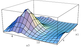
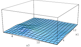
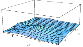
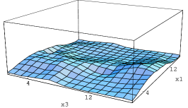
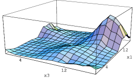
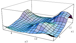
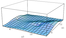
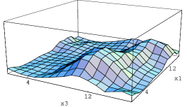
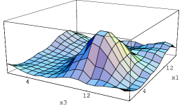
Figure 2: The lowest Laplacian mode in a thermalized background with $\zeta=0.02,0.355,0.48$ from left to right and in lattice planes $(x_{2},x_{4})=(12,1),(4,4),(6,3)$ from top to bottom. The vertical scale is 0.05.

In this subsection we explore the Laplacian modes as an analyzing tool on thermalized gauge field configurations. Fig. 2 shows the lowest-lying mode in a generic background obtained on a $16^{3}\cdot 4$ lattice at $\beta=2.2$ (which amounts to $T=0.75\,T_{c}$) confirming the expectation that these modes are free of UV fluctuations. We allow for a complex phase in the boundary condition, $\phi(x_{4}+N_{4})=\exp(2\pi i\zeta)\phi(x_{4})$ parametrised by an angle $\zeta\in[0,1/2]$ (the remaining $\zeta$’s can be mapped to this interval by charge conjugation). The ‘evolution’ of the Laplacian mode with this angle is shown vertically in Fig. 2, while the 3 rows represent different but fixed lattice planes, which contain the global maximum of the mode. In the example we find 3 lattice locations which become the global maximum within some $\zeta$-interval. Therefore, the lowest Laplacian mode in a thermalized background is hopping, too.

At the hopping points in $\zeta$ the value of the maximum as well as the inverse participation ratio (taking values between ${\rm IPR}=4$ and ${\rm IPR}=11$) decrease and the mode rearranges itself. For some boundary conditions the lowest Laplacian mode can be characterized as a global structure.

Analyzing 50 independent configurations the lowest mode hops up to four times as a function of $\zeta$. Apart from the Laplacian mode being wave-like, the hopping phenomenon resembles the behaviour of the fermion zero mode [8]. However, in both cases it is not obvious which gluonic feature, say in the topological charge, discriminates the preferred locations. Interestingly, we have found a correlation of the maximum of the periodic and antiperiodic Laplacian mode to positive and negative Polyakov loops, respectively. This is the same tendency as for calorons (see Fig. 1) which could be understood as an argument for calorons ‘underlying’ the quantum configuration. Alternatively, the Polyakov loop could play a role defining pinning centers for the Laplacian mode in the spirit of Anderson localisation in a random potential [9].

The lowest Laplacian mode in the adjoint representation we have found to have minima at the caloron monopoles (see also [1, 10]) that extend to two-dimensional sheets for antiperiodic boundary conditions. In thermalized backgrounds, the maxima of the adjoint modes are correlated to the fundamental ones with the same boundary condition, but are stronger localized than the latter.

3 A Fourier-like filter

Laplacian (‘harmonic’) eigenmodes can be used to define a new Fourier-like filter which we present now [4]. We were inspired by the representation of the field strength in terms of fermionic modes in [11], but here we aim to reconstruct directly the link variables on which any observable can be measured. To this end we combine the definition of the lattice Laplacian, Eq. (1), with a spectral decomposition and at $y=x+\hat{\mu}$ immediately obtain

$$U_{\mu}^{ab}(x)=-\sum_{n=1}^{\mathcal{N}}\lambda_{n}\phi^{a}_{n}(x)\phi^{*b}_{n}(x+\hat{\mu})\,,\qquad\mathcal{N}=N_{1}N_{2}N_{3}N_{4}\cdot 2$$ (2)

The idea is to truncate the sum on the right hand side of this equation at some $N\ll\cal{N}$. The question arises, how to relate such an expression to a unitary link variable. Here the charge conjugation helps, since it guarantees that every eigenvalue is two-fold degenerate with eigenfunction related as $\phi^{\prime a}(x)=\epsilon^{ab}\phi^{*b}(x)$. It follows that the corresponding bilinear expressions in Eq. (2) add up to an element of $SU(2)$ up to a factor. The same applies to the staple average in cooling or smearing. We divide by the square root of this factor, which is the determinant and positive for all practical purposes, and obtain the final filter formula

$$\tilde{U}_{\mu}^{ab}(x)_{N}=\left(-\sum_{n=1}^{N}\lambda_{n}\left[\phi^{a}_{n}(x)\phi^{*b}_{n}(x+\hat{\mu})-\epsilon^{ac}\phi^{c}_{n}(x)\phi^{*d}_{n}(x+\hat{\mu})\epsilon^{db}\,\right]\right)/\sqrt{\det(\ldots)}$$ (3)

The quality of the filter is controlled by $N$, where $N=\cal{N}$ reproduces the original configuration exactly. In the other extreme case, $N=1$, the filtered links $\tilde{U}_{\mu}(x)$ can be shown to be pure gauge. From the behaviour of $\phi^{a}(x)$ under gauge transformations it follows immediately that $\tilde{U}_{\mu}(x)$ transforms as a link (and no gauge fixing is involved in the filter).

The filtering can be performed with Laplacian modes of any boundary condition. Then Eq. (3) is just the average over opposite boundary conditions $\zeta$ and $-\zeta$. This additional parameter completely fixes the Polyakov loop at $N=1$ to ${\rm tr}\,\tilde{\mathcal{P}}(\vec{x})/2=\cos(2\pi\zeta)$, while for nontrivial cases $N\geq 2$ the Polyakov loop is observed to fluctuate around this value. It follows that in order to optimize the filter for our circumstances (confined phase, nontrivial holonomy calorons) the best choice is $\zeta=1/4$, i.e. halfway between periodic and antiperiodic boundary conditions.

Figure 3: Action and topological density and Polyakov loop of the caloron of Fig. 1 (left) filtered with $N=4$ (left, densities multiplied by 100) and $N=150$ (right, densities multiplied by 400) modes ($\zeta=1/4$).

In order to test the filter we again start with the caloron background. Fig. 3 shows the action and topological density as well as the Polyakov loop measured on the filtered links $\tilde{U}_{\mu}(x)$, to be compared with Fig. 1 (left). The filter with the number of modes as low as $N=4$ starts to reproduce the classical structures qualitatively, while for $N=150$ the agreement is almost perfect.

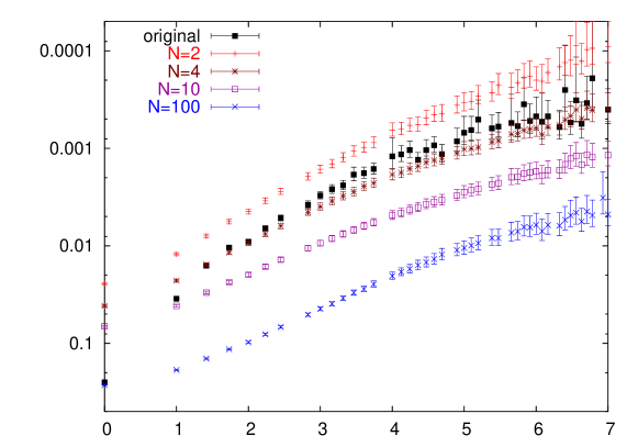
Figure 4: Polyakov loop correlator plotted on an inverse logarithmic scale over the distance for different $N$ (at $\zeta=1/4$) compared to the original one.

What is even more remarkable is that the filter method preserves the string tension. We plot the logarithm of the Polyakov loop correlator measured on 50 configurations at $T=0.75\,T_{c}$ in Fig. 4. It reveals a clearly linear behaviour with a slope reproducing the original one within 15%. The minimal number of modes, $N=2$, suffices for this behaviour. We conclude that the confining properties of lattice gauge theory are captured by the lowest Laplacian modes. The Polyakov loop correlator after filtering has no sign of a Coulomb regime, since the filter has washed out short range fluctuations. At zero distance the values $\langle({\rm tr}\,\tilde{\mathcal{P}}(\vec{x}))^{2}\rangle$ are smaller than the original one which indicates that the distribution of Polyakov loops over the lattice sites has become narrower.

Since the filter is not biased to classical solutions nor to particular degrees of freedom in the gauge field (like monopoles or vortices), it is interesting to have a closer look at the vacuum structures that emerge when the filter is applied to generic configurations. In both the Polyakov loop and the action density, more and more fluctuations appear with an increasing number of modes kept in the filter. It might well be that the fluctuation at $N=2$ are the minimally required ones for the long-range physics.

Concerning the action density, these objects are isolated peaks (which are non-static and not necessarily (anti)selfdual). This phenomenon is counterintuitive as the filter uses the lowest-lying Laplacian modes, however, this is also the case for the classical calorons, see Fig. 3 (left). We have found a correlation of the peak structure of the filtered action density to that emerging after cooling or smearing in an early stage. More work has to be done to better understand the ($N$-dependent) spiky structures induced by the filter.

References

- [1] F. Bruckmann, T. Heinzl, T. Vekua, and A. Wipf, Magnetic monopoles vs. Hopf defects in the Laplacian (Abelian) gauge, Nucl. Phys. B593 (2001) 545–561, [hep-th/0007119].
- [2] P. de Forcrand and M. Pepe, Laplacian gauge and instantons, Nucl. Phys. Proc. Suppl. 2001 (1994) 498–501, [hep-lat/0010093].
- [3] J. Greensite, Š. Olejník, M. I. Polikarpov, S. N. Syritsyn, and V. I. Zakharov, Localized eigenmodes of covariant Laplacians in the Yang-Mills vacuum, Phys. Rev. D71 (2005) 114507, [hep-lat/0504008].
- [4] F. Bruckmann and E.-M. Ilgenfritz, Laplacian modes probing gauge fields, hep-lat/0509020.
- [5] T. C. Kraan and P. van Baal, Periodic instantons with non-trivial holonomy, Nucl. Phys. B533 (1998) 627–659, [hep-th/9805168].
- [6] K. Lee and C. Lu, calorons and magnetic monopoles, Phys. Rev. D58 (1998) 025011, [hep-th/9802108].
- [7] M. García Pérez, A. González-Arroyo, C. Pena, and P. van Baal, Weyl-Dirac zero-mode for calorons, Phys. Rev. D60 (1999) 031901, [hep-th/9905016].
- [8] C. Gattringer and S. Schaefer, New findings for topological excitations in SU(3) lattice gauge theory, Nucl. Phys. B654 (2003) 30–60, [hep-lat/0212029].
- [9] P. W. Anderson, Absence of diffusion in certain random lattices, Phys. Rev. 109 (1958) 1492.
- [10] C. Alexandrou, M. D’Elia, and P. de Forcrand, The relevance of center vortices, Nucl. Phys. Proc. Suppl. 83 (2000) 437–439, [hep-lat/9907028].
- [11] C. Gattringer, Testing the self-duality of topological lumps in SU(3) lattice gauge theory, Phys. Rev. Lett. 88 (2002) 221601, [hep-lat/0202002].