Screening of sources in higher representations of SU(N) gauge theories at zero and finite temperature

Abstract:

Completion of the Svetitsky-Yaffe conjecture in some (2+1) dimensional SU(N) gauge theories allows mapping Polyakov loops in higher representations of the gauge group into suitable conformal operators of the corresponding 2D CFT. As a consequence, the critical exponents of the correlators of these Polyakov loops are determined. The functional form of these correlators suggests a general Ansatz to describe the large-distance screening of higher-representation sources at zero temperature in any space-time dimension. A generalised Wilson loop in which along part of its trajectory a source is converted in a gauge invariant way into higher representations with same $N-$ality could be used to estimate the decay scale of the unstable strings.

PoS(LAT2005)196

1 Introduction

The confining phase of $SU(N)$ gauge theory is characterised by a linear rising potential between static sources in the fundamental representation due to formation of a confining string joining these sources. It is natural to ask what is the potential between static sources in higher representations. One faces two somewhat related problems.

At $T=0$ two sources in a irreducible representation ${\cal R}$ and its conjugate $\bar{{\cal R}}$ give rise to the formation of a confining string with a string tension $\sigma_{\cal R}$. Most strings of this kind are expected to be unstable: if the representation ${\cal R}$ is built up of $j$ copies of the fundamental representation $f$, then $\sigma_{\cal R}$ should depend only on the $N$-ality of ${\cal R}$, defined as $k_{\cal R}\equiv j$ (mod $N$), because all representations with same $k$ can be converted into each other by the emission of a proper number of soft gluons, therefore the heavier ${\cal R}-$strings are expected to decay into the string with smallest string tension within the same $N$-ality. However this expectation seems not supported by numerical experiments. For a recent discussion on this subject see [1].

The other problem concerns the critical behaviour of the Polyakov lines in arbitrary representations at $T_{c}$. Universality arguments would, for continuous deconfining transitions, place the finite-temperature $SU(N)$ gauge theory in the universality class of $\mathbb{Z}_{N}$ invariant spin models in one dimension less [2]. The spin operator is mapped into the Polyakov line in the fundamental representation. What about the Polyakov lines in higher representations of $SU(N)$? There appears to be no room for independent exponents for these higher representations from the point of view of the abelian spin system. Also such an expectation seems not supported by numerical experiments (See [3] and references therein).

In this talk I describe a map between the operator product expansion (OPE) of the Polyakov operators in the gauge theory and the corresponding spin operators in the two-dimensional conformal field theory which describes the associated spin system at criticality which solves in some cases such an apparent puzzle and gives a hint to find a general solution of the related problem at $T=0$. A more detailed account of this approach as well as a complete list of references can be found in [4].

2 Polyakov loops at criticality

Consider a $2+1$ dimensional pure gauge theory undergoing a continuous deconfinement transition at the critical temperature $T_{c}$. The effective model describing the behaviour of Polyakov lines at finite $T$ will be a two-dimensional spin model with a global symmetry group coinciding with the center of the gauge group. According to the Svetitsky and Yaffe (SY) conjecture [2] such a spin model belongs in the same universality class of the original gauge theory.

Using the methods of conformal field theory (CFT), the critical behaviour can be often determined exactly. For example, the critical properties of $2+1$ dimensional $SU(3)$ gauge theory at deconfinement coincide with those of the 3-state Potts model,

What is needed to fully exploit the predictive power of the SY conjecture is a mapping relating the physical observables of the gauge theory to the operators of the dimensionally reduced model..

The correspondence between the Polyakov line in the fundamental representation $f$ and the order parameter $\sigma$ of the spin model is the first entry in this mapping:

$${\rm tr}^{~{}}_{f}(U_{\vec{x}})~{}\sim~{}\sigma(\vec{x})~{},$$ (1)

$U_{\vec{x}}$ is the gauge group element associated to the closed path wound once around the periodic imaginary time at the point $\vec{x}$. It is now natural to ask what operators in the CFT correspond to Polyakov lines in higher representations. On the gauge side, these can be obtained by a proper combination of products of Polyakov lines in the fundamental representation, using repeatedly the OPE of Polyakov operators in the fundamental representation:

$${\rm tr}^{~{}}_{f}(U_{\vec{x}})\;{\rm tr}\,_{f}(U_{\vec{y}})=\sum_{{\cal R}\in f\otimes f}C_{\cal R}(|\vec{x}-\vec{y}|)\,{\rm tr}^{~{}}_{{\cal R}}(U_{(\vec{x}+\vec{y})/2})+\dots$$ (2)

where the coefficients $C_{\cal R}(r)$ are suitable functions (they become powers of $r$ at the critical point) and the dots represent the contribution of higher dimensional local operators. The important property of this OPE is that the local operators are classified according to the irreducible representations of $G$ obtained by the decomposition of the direct product of the representations of the two local operators in the left-hand side.

On the CFT side, we have a similar structure. The order parameter $\sigma$ belongs to an irreducible representation $[\sigma]$ of the Virasoro algebra and the local operators contributing to an OPE are classified according to the decomposition of the direct product of the Virasoro representations of the left-hand-side operators. This decomposition is known as the fusion algebra.

In the case of three-state Potts model there is a finite number of representations, listed here along with their scaling dimensions

$${\mathbb{I}}~{}({\rm identity}); ~{}\sigma,\,\sigma^{+}~{}({\rm spin~{}fields});~{}\epsilon~{}({\rm energy});~{}\psi,\psi^{+}$$ (3)

$$x_{\mathbb{I}}=0; x_{\sigma}=\frac{2}{15};~{}~{}~{}~{}x_{\epsilon}=\frac{4}{15};~{}~{}~{}~{}~{}x_{\psi}=\frac{4}{3}~{}.$$ (4)

The fusion rule we need is

$$[\sigma]\star[\sigma]=[\sigma^{+}]+[\psi^{+}]~{};$$ (5)

Comparison of the first equation with the analogous one of the gauge side

$$\{3\}\otimes\{3\}=\{\bar{3}\}+\{6\}~{},$$ (6)

yields a new entry of the gauge/CFT correspondence

$${\rm tr}^{~{}}_{\{6\}}(U_{\vec{x}})~{}\sim~{}\psi^{+}(\vec{x})+c\,\sigma^{+}(\vec{x})~{},$$ (7)

where there are no a priori reasons for the vanishing of the coefficient $c$. Hence the Polyakov-Polyakov critical correlator of the symmetric representation $\{6\}$ is expected to have the following general form in the thermodynamic limit

$$\langle{\rm tr}^{~{}}_{\{6\}}(U_{\vec{x}})\;{\rm tr}^{~{}}_{\{\bar{6}\}}(U_{\vec{y}})\rangle_{SU(3)}^{~{}}=\frac{c_{s}}{r^{2x_{\sigma}}}+\frac{c_{u}}{r^{2x_{\psi}}}~{},$$ (8)

with $r=|\vec{x}-\vec{y}|$ and $c_{s},c_{u}$ suitable coefficients. Since $x_{\sigma}<x_{\psi}$, the second term drops off more rapidly than the first, thus at large distance this correlator behaves like that of the anti-symmetric representation $\{\bar{3}\}$ as expected also at zero temperature.

A similar reasoning can be applied to other representations of $SU(3)$ and $SU(4)$, as it has been explicitly worked out in Ref. [4].

3 Decay of unstable strings at zero temperature

The difficulty in observing string breaking or string decay with the Wilson loop seems to indicate nothing more than that it has a very small overlap with the broken-string or stable string state. Why? being a general phenomenon which occurs for any gauge group, including $\mathbb{Z}_{2}$, in pure gauge models as well as in models coupled to whatever kind of matter, it requires a general explanation which should not depend on detailed dynamical properties of the model. A simple, general, explanation in the case of gauge models coupled with matter was proposed in [6] and can be easily generalised to the present case [4] .

The general form of the Polyakov correlator in higher representations of $SU(3)$ found in Eq.s(8) suggests a simple Ansatz describing the asymptotic functional form of the vacuum expectation value of a large, rectangular, Wilson loop in a higher representation ${\cal R}$ coupled to an unstable string which should decay into a stable $k-$string

$$\langle W_{\cal R}(r,t)\rangle\simeq c_{u}\exp[-2\mu_{{\cal R}}^{~{}}(r+t)-\sigma_{{\cal R}}^{~{}}rt]+c_{s}\exp[-2\mu_{\cal R}^{\prime}(r+t)-\sigma_{k}^{~{}}rt]$$ (9)

The first term describes the typical area-law decay produced at intermediate distances by the unstable string with tension $\sigma_{{\cal R}}^{~{}}$. The second term is instead the contribution expected by the stable $k-$string in which the ${\cal R}-$string decays. In the case of adjoint representation (zero $N-$ality) one has $\sigma_{0}=0$ and the perimeter term $\mu^{\prime}_{adj}$ denotes the mass of the lowest glue-lump. Eq.(9) has to be understood as an asymptotic expansion which approximates $\langle W_{\cal R}(r,t)\rangle$ when $r,t>r_{o}$, where $r_{o}$ may be interpreted as the scale where the confining string forms.

When $t$ and $r$ are sufficiently large, no matter how small $c_{s}$ is, the above Ansatz implies that at long distances the stable string eventually prevails, since $\Delta\sigma\equiv\sigma_{\cal R}-\sigma_{k}>0$, hence the first term drops off more rapidly than the second and we have

$$V_{\cal R}(r)=V_{s}(r)=2\mu^{\prime}_{\cal R}+\sigma_{k}^{~{}}r~{},~{}~{}~{}r>r_{\cal R}^{~{}}~{},$$ (10)

where $V_{\cal R}(r)=-\lim_{t\to\infty}\frac{1}{t}\log\langle W_{\cal R}(r,t)\rangle$ is the static potential and $r_{\cal R}^{~{}}$ is the decay scale, given by

$$r_{\cal R}^{~{}}=\frac{2\Delta\mu}{\Delta\sigma}\equiv 2\frac{\mu^{\prime}_{\cal R}-\mu^{~{}}_{\cal R}}{\sigma^{~{}}_{\cal R}-\sigma^{~{}}_{k}}~{}.$$ (11)

In the case of zero $N-$ality the above equation yields the usual estimate of the adjoint string breaking scale. Notice that the mass $\mu_{\cal R}^{~{}}$ and $\mu^{\prime}_{\cal R}$ are not UV finite because of the additive self-energy divergences, which cannot be absorbed in a parameter of the theory. However, these divergences should cancel in their difference, hence $r^{~{}}_{\cal R}$ is a purely dynamical scale, defined for any non fully antisymmetric representation of $SU(N)$, which cannot be tuned by any bare parameter of the theory. When $r$ is less than t he decay scale $r^{~{}}_{\cal R}$ Eq.(10) is no longer valid and has to be replaced by

$$V_{\cal R}(r)=V_{u}(r)=2\mu^{~{}}_{\cal R}+\sigma_{\cal R}^{~{}}r~{},~{}~{}~{}r_{o}<r<r_{\cal R}^{~{}}~{}.$$ (12)

Thus, the Ansatz (9) describes the unstable string decay as a level crossing phenomenon, as already observed in the string breaking. From a computational point of view it is very challenging to check this Ansatz. As a matter of fact, only in 2+1 $SU(2)$ adjoint Wilson loop [5] and in in 2+1 $\mathbb{Z}_{2}$-Higgs model [6] the string breaking has been convincingly demonstrated in this way.

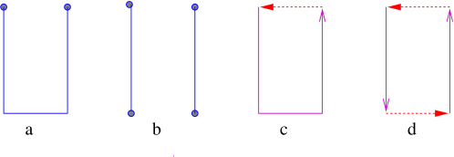
Figure 1: The operators depicted in $a$ and $b$ describe adjoint Wilson lines decaying in the vacuum. They are used to extract the adjoint static potential within the multichannel method. The mixed Wilson loops $c$ and $d$ generalise these operators to the case of representations of non zero $N-$ality.

4 Mixed Wilson loops

The winning move to easily observe the breaking of the adjoint string has been the proposal [7] of enlarging the basis of of the operators used to extract the potential. Adjoint sources, contrarily to what happens in the case of fundamental representation, can form gauge invariant open Wilson lines, like those depicted in Fig. 1 $a$ and $b$, having a good overlap with the broken adjoint string state. This suggests generalising such a construction to an excited irreducible representation ${\cal R}$ with non-vanishing $N$-ality $k$ by trying to construct operators as those depicted in Fig. 1 $c$ and $d$ where along one or more segments of the closed path $\gamma$ (the dashed lines in Fig.1) the static source carries the quantum numbers of ${\cal R}$, while in the remaining path (solid lines) the source lies in the stable, fully anti-symmetric representation $k$.

To construct such a mixed Wilson loop let us start by considering an arbitrary closed path $\gamma=u\,v$ made by the composition of two open paths $u$ and $v$. Let $U$ and $V$ be the group elements associated with these two paths respectively. The associated standard Wilson loop is

$$W_{f}(\gamma)={\rm tr}\,(UV)~{}.$$ (13)

where the trace is taken, here and in the following, in the fundamental representation $f$ of the non-abelian gauge group $G$. We want to transform $W$ in a mixed Wilson loop in which the source along the path $u$ carries the quantum numbers of an higher representation ${\cal R}$ belonging to the same $N-$ ality of $f$. To this end we perform the replacement

$$U\to UQU^{\dagger}PU$$ (14)

where $P$ and $Q$ are the group elements associated to two small loops inserted at the end points of the path $u$, in analogy with the “clovers” used in the construction of the glue-lump operator [7]. Along the path $u$ now propagates a source belonging to the reducible representation $f\otimes f\otimes\bar{f}$. We have then to project on some irreducible component. To make a specific, illustrative example, let us consider the case of $SU(3)$, where we have $\{3\}\otimes\{3\}\otimes\{\bar{3}\}=2\{3\}+\{\bar{6}\}+\{15\}$. We want to project on the $\{\bar{6}\}$ representation which has the same triality of $\{3\}$. It is easy to find

$$\begin{split}W^{~{}}_{\{3\}\to\{\bar{6}\}}(\gamma)=\frac{3}{2}\left[{\rm tr}\,(PUQU^{\dagger})\,{\rm tr}\,(VU)-{\rm tr}\,(PUVUQU^{\dagger})\right]+\\ \frac{3}{4}\left[{\rm tr}\,P\,{\rm tr}\,(VUQ)-{\rm tr}\,(VPUQ)+{\rm tr}\,(VPU)\,{\rm tr}\,Q-{\rm tr}\,P{\rm tr}\,(VU)\,{\rm tr}\,Q\,\right]~{}.\end{split}$$ (15)

Other examples and more details on the projections on the irreducible representations can be found in Ref.[4].

It is clear that the above construction can be generalised to any non-abelian group and, in particular, to any fully anti-symmetric representation of $N-$ality $k$ of $SU(N)$, which can be converted through the emission and the reabsorption of a glue-lump to an excited representation ${\cal R}$. It is also clear that one can build up mixed Wilson loops of the type drawn in Fig.1 $c$ and $d$ that we denote respectively as $W^{~{}}_{k\to{\cal R}}(r,t)$ and $W^{~{}}_{{\cal R}\to k\to{\cal R}}(r,t)$

The static potential $V_{\cal R}(r)$ between the ${\cal R}$ sources and the decay of the associated unstable string into the stable $k-$string can then be extracted in the standard way from measurements of the matrix correlator

$$C(r,t)=\left(\begin{matrix}\langle W^{~{}}_{{\cal R}}(r,t)\rangle&\langle W^{~{}}_{k\to{\cal R}}(r,t)\rangle\\ \langle W^{~{}}_{k\to{\cal R}}(r,t)\rangle&\langle W^{~{}}_{{\cal R}\to k\to{\cal R}}(r,t)\rangle\end{matrix}\right)~{},$$ (16)

where $W^{~{}}_{{\cal R}}$ is the ordinary Wilson loop when the whole rectangle $(r,t)$ is in the ${\cal R}$ representation. This is the generalisation of the multichannel method which has been used successfully to observe the breaking of the string in gauge theories coupled to matter fields as well as the adjoint string breaking. In this way we are confident that it will also possible to evaluate the decay scale $r_{\cal R}$.

One could also try to get a rough estimate of $r_{\cal R}$ through Eq.(11). Indeed the instability of the ${\cal R}-$string leads to conjecture that the vacuum expectation value of $W^{~{}}_{k\to{\cal R}}(\gamma)$ should behave asymptotically as

$$\langle W^{~{}}_{k\to{\cal R}}(\gamma)\rangle\propto e^{-\mu_{\cal R}^{~{}}|v|-\mu_{\cal R}^{\prime}|u|-\sigma^{~{}}_{k}A}~{},$$ (17)

where $A$ is the area of the minimal surface encircled by $\gamma$ and $|v|$ and $|u|$ are the lengths of the paths which carry the quantum numbers of the representations $k$ and ${\cal R}$, respectively. This seems the most effective way to estimate the quantity $\mu^{\prime}_{\cal R}$ and therefore $r^{~{}}_{\cal R}$.

References

- [1] A. Armoni and M. Shifman, Remarks on stable and quasi-stable k-strings at large N, Nucl. Phys.B 671 (2003) 67 [hep-th/0307020].
- [2] B. Svetitsky and L.G. Yaffe, Critical behaviour at finite temperature confinement transitions, Nucl. Phys. B 210 [FS6] (1982) 423.
- [3] P.H. Damgaard and M. Hasenbusch, Screening and deconfinement of sources in finite temperature SU(2) lattice gauge theory, Phys. Lett. B 331 (1994) 400 [hep-lat/9404008].
- [4] F. Gliozzi, The decay of unstable k-strings in SU(N) gauge theories at zero and finite temperature, JHEP 08 (2005)063 [hep-th/0507016].
- [5] S.Kratochvila and P.de Forcrand, Observing string breaking with Wilson loops, Nucl. Phys. B 671 (2003) 103 [hep-lat/0306011].
- [6] F. Gliozzi and A. Rago, Overlap of the Wilson loop with the broken-string state, Nucl. Phys. B 714 (2005) 91 [hep-lat/0411004].
- [7] C. Michael, Hadronic forces from the lattice, Nucl Phys. B 26 (Proc. Suppl.) (1992) 417.