Restoring chiral symmetry to $\mathrm{O}(a^{2})$ for dynamical Wilson fermions

Abstract:

We present results for the non–perturbative determination of the improvement and renormalization factors of the isovector axial current for lattice QCD with two flavors of dynamical Wilson quarks. The improvement and normalization conditions are formulated in terms of matrix elements of the PCAC relation in the Schrödinger functional setup and results are given in the form of interpolating formulae for bare gauge couplings $\beta=6/g_{0}^{2}>5.2$.
Work supported by the DFG in the Graduiertenkolleg GK271 and the SFB/TR 09-03.

PoS(LAT2005)232

1 Introduction

With the Wilson fermion formulation chiral symmetry is explicitly broken at finite lattice spacing and the consequences of this explicit breaking have to be dealt with. Among those is the fact that $\mathrm{O}(a)$ counter terms in the Symanzik expansion are no longer excluded and that there is no conserved Noether current associated with a continuous chiral symmetry of the lattice action.

The first problem is addressed by the Symanzik improvement programme, i.e. the addition of irrelevant operators to both the action and the composite fields. By tuning the coefficients of only a few terms it is possible to remove the $\mathrm{O}(a)$ scaling violations from the theory. Here we compute the improvement coefficient for the isovector axial current $c_{\rm A}(g_{0}^{2})$, which – together with the improvement of the action [1] – will ensure the absence of $\mathrm{O}(a)$ lattice artifacts in all matrix elements of the PCAC relation, which involve insertions at finite separation [2].

The normalization factor $Z_{\rm A}(g_{0}^{2})$ of the improved axial current is obtained by enforcing a continuum–like transformation behavior under infinitesimal chiral rotations. Since the isovector chiral symmetry is recovered in the continuum and the normalization condition is based on a local identity, $Z_{\rm A}$ is finite and scale–independent.

For unexplained notation and additional details about the improvement and normalization conditions we refer to [3] and [4], respectively.

2 Axial current improvement

When calculating a bare quark mass on the lattice from matrix elements of the PCAC relation

$$\partial_{\mu}A^{a}_{\mu}(x)=2mP^{a}(x)\;,$$ (1)

any dependence on the kinematic parameters or external states, i.e. the dependence on the precise choice of matrix element, is a cutoff effect. A non–perturbative improvement condition can thus be obtained by inserting into eq. (1) the improved axial current [2]

$$(A_{\rm I})_{\mu}^{a}(x)=A_{\mu}^{a}(x)+ac_{\rm A}{\textstyle\frac{1}{2}}(\partial_{\mu}+\partial^{*}_{\mu})P^{a}(x)\;,$$ (2)

and tuning $c_{\rm A}$ such that the masses obtained from two different matrix elements agree. In (2) $\partial_{\mu}$ ($\partial_{\mu}^{*}$) denotes the forward (backward) lattice derivative.

When evaluating improvement coefficients non–perturbatively one has to keep in mind that due to cutoff effects in the correlation function used to formulate the improvement condition, the coefficients themselves are uncertain to $\mathrm{O}(a)$. While this forbids a unique definition of the improved theory, the $\mathrm{O}(a)$ ambiguities can be made to disappear smoothly if the improvement condition is evaluated with all physical scales kept fixed, while only the lattice spacing is varied [5]. In the evaluation of our improvement condition we keep the bare quark mass (using the 1–loop value for $c_{\rm A}$ from [6]) constant, thus ignoring small changes in renormalization factors, and fix the relative lattice spacing in the range of bare gauge couplings we consider through asymptotic scaling [3].

It is also important to make sure that the correlation functions in the improvement condition are not dominated by states with energy close to the cutoff. If this were the case, the improvement condition might cancel exceptionally large scaling violations and a $c_{\rm A}$ obtained in this way could introduce significant $\mathrm{O}(a^{2})$ effects.

We construct matrix elements of (1) between pseudo–scalar states and the vacuum in the Schrödinger functional [7, 8]. More precisely, in this work we use

$$f_{\rm A}(x_{0};\omega) = -\frac{a^{3}}{3L^{6}}\sum_{\bf x}\langle A_{0}^{a}(x)\,\mathcal{O}^{a}(\omega)\rangle\;,$$ (3)

$$\textrm{and }\ \ f_{\rm P}(x_{0};\omega) = -\frac{a^{3}}{3L^{6}}\sum_{\bf x}\langle P^{a}(x)\,\mathcal{O}^{a}(\omega)\rangle\;,$$ (4)

with the pseudo–scalar operator

$$\quad\mathcal{O}^{a}(\omega)=a^{6}\sum_{{\bf x},{\bf y}}\bar{\zeta}({\bf x})\gamma_{5}\tau^{a}{\textstyle\frac{1}{2}}\omega({\bf x}-{\bf y})\zeta({\bf y})\;.$$ (5)

It lives at the $x_{0}\!=\!0$ boundary of the SF cylinder and depends on a spatial trial “wave function” $\omega$. A quark mass from (1) using (2) is then given by $m=r+ac_{\rm A}s+\mathrm{O}(a^{2})$ with

$$r(x_{0};\omega)=\frac{{\textstyle\frac{1}{2}}(\partial_{0}+\partial^{*}_{0})f_{\rm A}(x_{0};\omega)}{2f_{\rm P}(x_{0};\omega)}\quad \quad s(x_{0};\omega)=\frac{\partial_{0}\partial^{*}_{0}f_{\rm P}(x_{0};\omega)}{2f_{\rm P}(x_{0};\omega)}\;.$$ and (6)

In our chosen setup we now have $x_{0}$, the insertion time, and $\omega$, the spatial trial wave function, as parameters for probing the PCAC relation. Enforcing the independence of the quark mass from these results in

$$-c_{\rm A}=\frac{\Delta r}{a\Delta s}=\frac{1}{a}\!\cdot\!\frac{r(x_{0};\omega_{\pi,1})-r(y_{0};\omega_{\pi,0})}{s(x_{0};\omega_{\pi,1})-s(y_{0};\omega_{\pi,0})}\;,$$ (7)

and therefore the sensitivity to $c_{\rm A}$ is given by $a\Delta s$.

The combined requirement of large sensitivity to $c_{\rm A}$ and explicit control over excited–state contributions is met with the method proposed in [9] where it is tested in the quenched approximation. There $\omega_{\pi,0/1}$ from (7) are chosen such that $\mathcal{O}(\omega_{\pi,0/1})$ excite mostly the ground and first excited state in the pseudo–scalar channel, respectively. Thus the energy of the states can be monitored directly using the effective mass of $f_{\rm A/P}$ and the sensitivity $a\Delta s=as(x_{0},\omega_{\pi,1})-as(x_{0},\omega_{\pi,0})\propto{m_{\pi}^{\star}}^{2}-m_{\pi}^{2}$ is also expected to be large.

The simulations listed in Table 2 are at constant physical volume according to asymptotic scaling as described in [3] and the bare (unimproved) PCAC mass is kept constant to $\simeq 10\%$. [htb]—llll—$L/a$ $\beta$ $\ m\cdot L$ $-c_{\rm A}$
12 5.20 $0.18(1)$ 0.0638(23)
16 5.42 $0.200(5)$ 0.0420(21)
24 5.70 $0.182(5)$ 0.0243(36)
Simulation parameters for $c_{\rm A}$. We simulate a set of three spatial wave functions and approximate the combinations $\mathcal{O}(\omega_{\pi,0/1})$ that project to the ground and first excited states through the eigenvectors of the correlation matrix [9, 3]

$$f_{1}(\omega^{\prime},\omega) = -\frac{1}{3L^{6}}\langle\mathcal{O}^{\prime a}(\omega^{\prime})\,\mathcal{O}^{a}(\omega)\rangle\;,$$ (8)

where $\mathcal{O}^{\prime}$ is a pseudo–scalar operator at the $x_{0}=T$ boundary. In Fig. 2 two distinct signals are clearly visible, which indicates that the approximate projection method works well at our parameters. The energy of the first excited state is not far away from $a^{-1}$, suggesting that in even smaller volumes the residual $\mathrm{O}(a^{2})$ effects would grow rapidly.

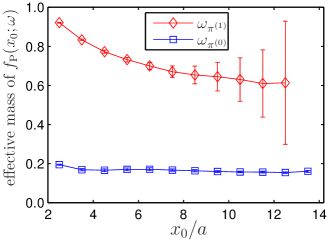
Figure 1: Effective pseudo–scalar masses of $f_{\rm P}$ from the $\beta=5.42$ run.

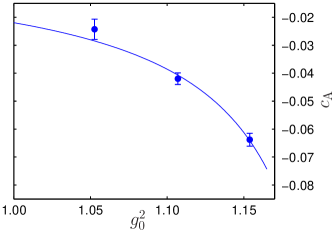
Figure 2: Simulation results for $c_{\rm A}$. The solid line is given by the interpolating formula (9).

Our definition of $c_{\rm A}$ is completed by fixing $x_{0}=y_{0}=T/2$ in (7) and specifying $L=T$ and $\theta=0$. The results from the simulations summarized in Table 2 are shown in Fig. 2 as a function of $g_{0}^{2}$. The solid line is a smooth interpolation of the simulation data, constrained in addition by 1–loop perturbation theory:

$$c_{\rm A}(g_{0}^{2})=-0.00756\,g_{0}^{2}\times\frac{1-0.4485\,g_{0}^{2}}{1-0.8098\,g_{0}^{2}}\;.$$ (9)

It is our final result, valid in the range $0.98\leq g_{0}^{2}\leq 1.16$ within the errors of the data points (at most 0.004). By performing additional simulations we have verified that the volumes in our runs are scaled sufficiently precisely such that systematic errors due to deviations from the constant physics condition can be neglected. The same also applies to variations in the quark mass.

3 Axial current renormalization

In a massless renormalization scheme preservation of $\mathrm{O}(a)$–improvement implies that the renormalized improved current is of the form [10, 2]

$$(A_{\rm R})_{\mu}^{a}=Z_{\rm A}(1+b_{\rm A}m_{\rm q})(A_{\rm I})_{\mu}^{a}\;.$$ (10)

The normalization condition we use [11, 4] is based on [12], the ALPHA collaboration’s quenched determination of $Z_{\rm A}$. Since a massless scheme requires the normalization condition to be set up at vanishing quark mass, in [12] the mass term of the axial Ward identity was dropped in the derivation of the normalization condition. In practice this condition shows a very pronounced quark mass dependence and thus a potential extrapolation is rather steep and the location of the critical point must be known with high precision.

Performing a chiral transformation in the continuum and keeping track of the mass term results in the integrated Ward identity [4]

$$\int\!\!{\rm d}^{3}{\bf y}\,{\rm d}^{3}{\bf x}\,\epsilon^{abc}\Big{\langle}A_{0}^{a}(y_{0}\!+\!t,{\bf x})A_{0}^{b}(y)\mathcal{O}_{\rm ext}\Big{\rangle}\qquad\qquad$$

$$-2m\!\int\!\!{\rm d}^{3}{\bf y}\,{\rm d}^{3}{\bf x}\!\int_{y_{0}}^{y_{0}+t}\!\!\!\!\!{\rm d}x_{0}\,\epsilon^{abc}\Big{\langle}P^{a}(x)A_{0}^{b}(y)\mathcal{O}_{\rm ext}\Big{\rangle} \!=\! i\displaystyle\!\int\!\!{\rm d}^{3}{\bf y}\ \Big{\langle}V_{0}^{c}(y)\mathcal{O}_{\rm ext}\Big{\rangle}\;\qquad$$ (11)

and the choice $\mathcal{O}^{c}_{\rm ext}=-\epsilon^{cde}\mathcal{O}^{\prime d}\mathcal{O}^{e}/{6L^{6}}$ allows us to replace the r.h.s. of (11) with $f_{1}$ by using isospin symmetry. A normalization condition is then obtained by requiring that (11) holds for the renormalized improved current (10).

Fig. 4 shows the results of an evaluation of this condition at a bare gauge coupling of $\beta=5.2$. To show the effect of the inclusion of the mass term, also the results with the method from [12] are shown, i.e. when dropping the second term on the l.h.s. of (11). While for the new normalization condition the slope in $am$ is consistent with zero, the estimate of $Z_{\rm A}$ from the old condition changes by $30\%$ in the (small) mass range shown. We anyway see that for $am\lesssim 0.02$ all mass effects show a linear behavior. For $\beta=5.5$ the extrapolation is similar to the one shown and at all other gauge couplings we can in fact interpolate from two simulations very close to the critical point. [b]—c—rrll— $\beta$ $L/a$ $T/a$ $\kappa_{c}\qquad$ $Z_{\rm A}\qquad$  
5.200 8 18 0.135856(18) 0.7141(123)
5.500 12 27 0.136733(8) 0.7882(35)(39)
5.715 16 36 0.136688(11) 0.8037(38)(7)
5.290 8 18 0.136310(22) 0.7532(79)
7.200 8 18 0.134220(21) 0.8702(16)(7)
8.400 8 18 0.132584(7) 0.8991(25)(7)
9.600 8 18 0.131405(3) 0.9132(11)(7)
Results for the chiral extrapolations of $Z_{\rm A}$ and estimates for the critical hopping parameter $\kappa_{c}$. In addition to three (again asymptotically) matched lattice sizes at $L/a=8,12$ and $16$, we simulated at three larger values of $\beta$ and fixed $L/a=8$, which corresponds to very small volumes. This was done in order to verify that our non–perturbative estimate smoothly connects to the perturbative predictions [13, 14]. The first error we quote for $Z_{\rm A}$ is statistical and the second represents our estimate of the systematic error, which originates from deviations from the constant physics condition.

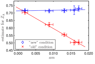
Figure 3: Comparison of the chiral extrapolation at $\beta=5.2$ using the new and old normalization conditions for $Z_{\rm A}$.

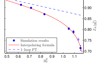
Figure 4: Result for $Z_{\rm A}$ from numerical simulations and 1–loop perturbation theory (dashed line). The Pade fit (solid lines) is given by (12).

There is no estimate of the systematic error for the $\beta=5.29$ run, which was done only to verify the rapid change of $Z_{\rm A}$ in this region of bare gauge coupling. It is thus also excluded from a fit, which results in the interpolating formula (again incorporating the 1–loop asymptotic constraint)

$$Z_{\rm A}(g_{0}^{2})=\frac{1-0.918\,g_{0}^{2}+0.062\,g_{0}^{4}+0.020\,g_{0}^{6}}{1-0.8015\,g_{0}^{2}}\;.\\$$ (12)

4 Summary and Outlook

For the $\mathrm{O}(a)$-improved action with non-perturbative $c_{\rm SW}$ [1], we have determined the improvement coefficient $c_{\rm A}$ for $\beta\!\geq\!5.2$, which roughly corresponds to $a\!\leq\!0.1$ fm. The improvement condition was implemented at constant physics, which is necessary in a situation when $\mathrm{O}(a)$ ambiguities in the improvement coefficients are not negligible.

Through the calculation of $Z_{\rm A}(g_{0}^{2})$ we have shown that in a lattice theory with two flavors of Wilson fermions normalization conditions can be imposed at the non–perturbative level such that isovector chiral symmetries are realized in the continuum limit. Since we are working with an improved theory, chiral Ward–Takahashi identities are then satisfied up to $\mathrm{O}(a^{2})$ at finite lattice spacing.

The improvement and normalization conditions were implemented in terms of correlation functions in the Schrödinger functional framework and evaluated on a line of constant physics in order to achieve a smooth disappearance of the $\mathrm{O}(a)$ and $\mathrm{O}(a^{2})$ uncertainties. Clearly, the methods employed in this paper may also be useful to compute $c_{\rm A}$ and $Z_{\rm A}$ in the three flavor case, where $c_{\rm SW}$ is known non–perturbatively with plaquette and Iwasaki gauge actions [15, 16, 17].

The determinations of $c_{\rm A}$ and $Z_{\rm A}$ were carried out within the ALPHA collaboration’s programme to calculate quark masses in a fully non–perturbative framework. The results of this programme and its application to the strange quark mass are presented in [18, 19].

References

- [1] ALPHA Collaboration, K. Jansen and R. Sommer, Nucl. Phys. B530 (1998) 185–203 [hep-lat/9803017].
- [2] M. Lüscher, S. Sint, R. Sommer and P. Weisz, Nucl. Phys. B478 (1996) 365–400 [hep-lat/9605038].
- [3] ALPHA Collaboration, M. Della Morte, R. Hoffmann and R. Sommer, JHEP 03 (2005) 029 [hep-lat/0503003].
- [4] ALPHA Collaboration, M. Della Morte, R. Hoffmann, F. Knechtli, R. Sommer and U. Wolff, JHEP 07 (2005) 007 [hep-lat/0505026].
- [5] ALPHA Collaboration, M. Guagnelli et. al., Nucl. Phys. B595 (2001) 44–62 [hep-lat/0009021].
- [6] M. Lüscher and P. Weisz, Nucl. Phys. B479 (1996) 429–458 [hep-lat/9606016].
- [7] M. Lüscher, R. Narayanan, P. Weisz and U. Wolff, Nucl. Phys. B384 (1992) 168–228 [hep-lat/9207009].
- [8] S. Sint, Nucl. Phys. B421 (1994) 135–158 [hep-lat/9312079].
- [9] S. Dürr and M. Della Morte, Nucl. Phys. Proc. Suppl. 129 (2004) 417–419 [hep-lat/0309169].
- [10] K. Jansen et. al., Phys. Lett. B372 (1996) 275–282 [hep-lat/9512009].
- [11] R. Hoffmann, F. Knechtli, J. Rolf, R. Sommer and U. Wolff, Nucl. Phys. Proc. Suppl. 129 (2004) 423–425 [hep-lat/0309071].
- [12] M. Lüscher, S. Sint, R. Sommer and H. Wittig, Nucl. Phys. B491 (1997) 344–364 [hep-lat/9611015].
- [13] E. Gabrielli, G. Martinelli, C. Pittori, G. Heatlie and C. T. Sachrajda, Nucl. Phys. B362 (1991) 475–486.
- [14] M. Göckeler et. al., Nucl. Phys. Proc. Suppl. 53 (1997) 896–898 [hep-lat/9608033].
- [15] CP-PACS Collaboration, S. Aoki et. al., Nucl. Phys. Proc. Suppl. 119 (2003) 433–435 [hep-lat/0211034].
- [16] JLQCD Collaboration, N. Yamada et. al., hep-lat/0406028.
- [17] CP-PACS Collaboration, S. Aoki et. al., hep-lat/0508031.
- [18] ALPHA Collaboration, M. Della Morte, R. Hoffmann, F. Knechtli, J. Rolf, R. Sommer, I. Wetzorke and U. Wolff, hep-lat/0507035.
- [19] M. Della Morte et. al., PoS (LAT2005) 233 [hep-lat/0509073].