Towards a non-perturbative computation of the RGI strange quark mass with two dynamical flavors

Abstract:

The non-perturbative running of the quark mass in the Schrödinger functional scheme is computed over a large energy range (covering scales differing by two orders of magnitude). This allows to relate lattice estimates of the running quark mass to the renormalization group invariant mass. The result is used in a preliminary computation of the strange quark mass in the theory with two flavors of non-perturbatively improved Wilson quarks. A more detailed discussion of the calculation can be found in [1].

PoS(LAT2005)233

1 Introduction

Quark masses are parameters of QCD. They can be computed non-perturbatively on the lattice once an hadronic input is given. Sticking to the renormalization group invariant (RGI) definition of the quark mass, lattice results for the strange quark mass with 2 [2, 3, 4] and 2+1 [5, 6] dynamical flavors differ among each other by more than 40 MeV. Such a spread can be ascribed to various systematics, mainly cutoff effects and the renormalization procedure, which in many cases relies on perturbation theory only. For the result we will present here the renormalization is performed in a fully non-perturbative way, while the lattice spacing is still varied in a small range only (roughly 0.1 to 0.07 fm).

We write the relation among the bare current (PCAC) quark mass $m_{i}$ and the RGI mass $M_{i}$ as

$$M_{i}=Z_{\rm M}(g_{0})\,m_{i}(g_{0})\,,$$ (1)

where $i$ has to be interpreted as a flavor index. The factor $Z_{\rm M}$ can be split into two parts, the first one connecting the bare mass to $\overline{m}_{i}(\mu)$, the renormalized one (in the Schrödinger functional scheme) at a given scale $\mu$

$$\overline{m}_{i}(\mu)={Z_{\rm A}(g_{0})\over Z_{\rm P}(g_{0},a\mu)}\,m_{i}(g_{0})\,,$$ (2)

and the second one $M/\overline{m}(\mu)$, which relates two renormalized masses and is therefore universal. In mass independent schemes (like the one we are going to describe) this second factor is also flavor independent [7]. Its computation is the main result we report about here.

The renormalization group equations for the couplings are decoupled in mass independent schemes and read

$$\mu\frac{{\rm d}\bar{g}}{{\rm d}\mu}=\beta(\bar{g})\quad,\quad\mu\frac{{\rm d}\overline{m}_{i}}{{\rm d}\mu}=\tau(\bar{g})\overline{m}_{i}\,.$$ (3)

with $\bar{g}(\mu)$ the renormalized coupling at the scale $\mu$. The $\tau$ and $\beta$ functions can be expanded in perturbation theory

$$\beta(\bar{g})_{\mbox{$\stackrel{{\scriptstyle\displaystyle\sim}}{{\scriptstyle\bar{g}\rightarrow 0}}$}}-\bar{g}^{3}\{b_{0}+b_{1}\bar{g}^{2}+b_{2}\bar{g}^{4}+...\}\quad,\quad\tau(\bar{g})_{\mbox{$\stackrel{{\scriptstyle\displaystyle\sim}}{{\scriptstyle\bar{g}\rightarrow 0}}$}}-\bar{g}^{2}\{d_{0}+d_{1}\bar{g}^{2}+...\}\,,$$ (4)

and the exact (i.e. valid beyond perturbation theory) solutions of eqs. (3) can be written

$$\Lambda = \mu(b_{0}\bar{g}^{2})^{-b_{1}/2b_{0}^{2}}{\rm e}^{-1/(2b_{0}\bar{g}^{2})}\exp\left\{-\int_{0}^{\bar{g}}{\rm d}x\left[\frac{\displaystyle{1}}{\displaystyle{\beta(x)}}+\frac{\displaystyle{1}}{\displaystyle{b_{0}x^{3}}}-\frac{\displaystyle{b_{1}}}{\displaystyle{b_{0}^{2}x}}\right]\right\}\,,$$ (5)

$$M_{i} = \overline{m}_{i}(2b_{0}\bar{g}^{2})^{-d_{0}/2b_{0}}\exp\left\{-\int_{0}^{\bar{g}}{\rm d}x\left[\frac{\displaystyle{\tau(x)}}{\displaystyle{\beta(x)}}-\frac{\displaystyle{d_{0}}}{\displaystyle{b_{0}x}}\right]\right\}\,,$$ (6)

where the RGI parameters $\Lambda$ and $M$ appear as integration constants. At the level of RGI parameters the connections among different schemes can be given in a simple and exact way. We thus regard them as the fundamental parameters of QCD.

2 Running of the quark mass in the SF scheme

In terms of Schrödinger functional (SF) correlation functions the bare PCAC mass reads

$$m(g_{0},\kappa)=\left.\frac{\frac{1}{2}(\partial_{0}^{\ast}+\partial_{0})f_{\rm A}(x_{0})+c_{\rm A}a\partial_{0}^{\ast}\partial_{0}f_{\rm P}(x_{0})}{2f_{\rm P}(x_{0})}\right|_{x_{0}=T/2}\;,$$ (7)

where $\kappa$ is the hopping parameter. We use the plaquette gauge action and non-perturbatively O($a$) improved Wilson fermions [8]. The improvement coefficient $c_{\rm A}$ is also set to its non-perturbative value from [9]. For the definition of the SF with Wilson fermions we refer to [10] and to [11] for any unexplained notation. Here we only recall that the correlation functions $f_{\rm A}$ and $f_{\rm P}$ involve matrix elements of the axial current and the pseudoscalar density operators, respectively. According to eq. (2) the running quark mass at the scale $\mu$ is obtained by multiplying the mass in eq. (7) by the ratio $Z_{\rm A}(g_{0})/Z_{\rm P}(g_{0},a\mu)$. The factor $Z_{\rm A}$ is scale independent and can be fixed by Ward identities [12]. All the scale dependence in the running quark mass comes from $Z_{\rm P}$. In the SF it can be defined as

$$Z_{\rm P}(g_{0},L/a)=c{{\sqrt{3f_{1}}}\over f_{\rm P}(L/2)}\;,\quad m=0,\;\;\theta=0.5,\;\;T=2L\;,$$ (8)

where the boundary to boundary correlation function $f_{1}$ takes care of the renormalization of the boundary quark fields and the constant $c$ ensures $Z_{\rm P}=1$ at tree level. Eq. (8) makes clear that in the finite volume scheme we are using, the normalization scale $\mu$ is identified with the (inverse) extent of the system, which, in turn, is uniquely fixed (up to cutoff effects) by the value of the running coupling $\bar{g}^{2}(L)$. The non perturbative running of the quark mass is described by the step scaling function $\sigma_{\rm P}(u)$

$$\sigma_{\rm P}(u)={{\overline{m}(\mu)}\over{\overline{m}(\mu/2)}}=\lim_{a\rightarrow 0}\left.{{Z_{\rm P}(g_{0},2L/a)}\over{Z_{\rm P}(g_{0},L/a)}}\right|_{\bar{g}^{2}(L)=u}\;,$$ (9)

which can be viewed as an integrated form of the $\tau$ function. Introducing also the step scaling function for the coupling $\sigma(u)=\bar{g}^{2}(L)$ (computed in [13]) and solving the following coupled recursions

$$\left\{\begin{array}[]{l}u_{0}=\bar{g}^{2}(L_{\rm max})=4.61\\ \sigma(u_{k+1})=u_{k}\end{array}\right. \Rightarrow u_{k}=\bar{g}^{2}(L_{k})\,,\quad L_{k}=2^{-k}L_{\rm max}\,,$$ (12)

$$\left\{\begin{array}[]{l}w_{0}=1\\ w_{k}=\left[\prod_{i=1}^{k}\sigma_{\rm P}(u_{i})\right]^{-1}\end{array}\right. \Rightarrow w_{k}=\frac{\overline{m}(1/L_{\rm max})}{\overline{m}(1/L_{k})}\,,$$ (15)

starting from the low energy scale $1/L_{\rm max}$ defined by $u_{0}\,=\,\bar{g}^{2}(L_{\rm max})=4.61$ to the higher scales $1/L_{k}$, $k=0,1,\ldots,8$ (with $L_{0}\equiv L_{\rm max}$), one can obtain the ratio $\frac{\overline{m}(1/L_{\rm max})}{\overline{m}(1/L_{k})}$. For $k\geq 6$ contact can be made with perturbation theory, in such a way that the RGI parameters can be computed from eqs. (5, 6) by using the 2-loop $\tau$ function and 3-loop $\beta$ function.

In practice we calculated $\sigma_{\rm P}(u)$ at 6 different couplings in the range $u=3.33\dots 0.98$, extrapolating to the continuum limit lattice results from resolutions $L/a=6,$ 8 and 12 (see [1] for details about the extrapolations). The change in scale by a factor 2 needed for $\sigma$ and $\sigma_{\rm P}$ is “easily” implemented in the SF scheme as it amounts to doubling $L/a$ at fixed bare parameters (in other words we used lattices with $L/a$ up to 24). We parameterize the results by the ansatz

$$\sigma_{\rm P}(u)=1-\ln(2)d_{0}u+p_{1}u^{2}+p_{2}u^{3}\;,$$ (16)

with free coefficients $p_{1}$ and $p_{2}$. Inserting it in the recursion eq. (15), for the case $k=6$, we obtain

$$\frac{M}{\overline{m}(\mu)}=1.297(16)\quad\mbox{at}\quad\mu\,=\,1/L_{\rm max}\,.$$ (17)

Using the result for $L_{\rm max}\Lambda$ from [13], we plot in figure 1 the running of the quark mass versus $\mu/\Lambda$. In the plot we only include the errors from the coefficients $w_{k}$; the uncertainties on $\Lambda$ and $M$ would simply amount to a shift of the axes.

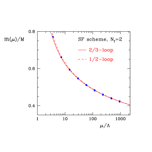
Figure 1: The non–perturbative running of $\overline{m}$. 2/3–loop refers to the 2–loop $\tau$-function and 3–loop $\beta$–function, analogously 1/2–loop.

The figure shows that in this case perturbation theory works surprisingly well down to rather small energies. This property is anyway specific of the quantity and the scheme considered here. As an example, the non-perturbative $\beta$ function in the SF scheme shows larger deviations from perturbation theory at the lower end of energies reached here [13].

3 The strange quark mass

In order to apply the described procedure to the computation of the strange quark mass we first need to calculate the factor $Z_{\rm A}(g_{0})/Z_{\rm P}(g_{0},L_{\rm max}/a)$ for the bare couplings (i.e. lattice spacings) used in large volume simulations. As we are going to use results from [4], the relevant set of $\beta$ values is 5.2, 5.29 and 5.4. Since this region is covered by the result for $Z_{\rm A}(g_{0})$ (and for $Z_{\rm A}^{\rm con}$, see figure 2) in [12], it remains to compute $Z_{\rm P}(g_{0},L_{\rm max}/a)$. At $\beta=5.2$ the value is directly obtained by a simulation at $L/a=6$ while at the other couplings we had to interpolate the results from different $L/a$ (the appropriate one wouldn’t have been an integer). The numbers are collected in table 1. Clearly now $Z_{\rm P}$ and $Z_{\rm M}$ refer to the chosen discretization, whereas the ratio in eq. (17) is universal.

$\beta$	$Z_{\rm P}$	$Z_{\rm M}$
5.20	0.47876(47)	1.935(33)(24)
5.29	0.4936(34)	1.979(25)(24)
5.40	0.4974(33)	2.001(29)(25)

Table 1: Results for $Z_{\rm P}$ and $Z_{\rm M}$ for three coupling values.

As we work with two degenerate flavors, instead of the strange quark mass what we actually compute is $M_{\rm ref}$ associated with a kaon made from two degenerate quarks. We use data for $r_{0}(\kappa)$ and $m_{\rm PS}(\kappa)$ from [4]. After extrapolating $r_{0}(\kappa)$ to the chiral limit (i.e to $\kappa=\kappa_{c}$) we fit the product $r_{0}(\kappa_{c})m_{\rm PS}(\kappa)$ as a function of $\kappa$ in order to determine $\kappa_{\rm ref}$ defined such that

$$(r_{0}(\kappa_{c})m_{\rm PS}(\kappa_{\rm ref}))^{2}=(r_{0}m_{\rm K})^{2}=1.5736\;,$$ (18)

where we have used $r_{0}=0.5\;$ fm [15]. Finally we compute the PCAC masses at the bare parameters $\beta,\kappa_{\rm ref}(\beta)$ with $\beta=$5.2, 5.29 and 5.4 in volumes of approximately 1.5 fm. This reduces cutoff effects in the PCAC mass due to finite size [16]. The result for the RGI quantity is

$$M_{\rm ref}=72(3)(13)\;{\rm MeV}\;,$$ (19)

the first error is statistical, the second is our estimate of cutoff effects obtained by comparing the result at the finest lattice spacing with that at the coarsest one. The number in eq. (19) is consistent with the quenched estimate of the same quantity [11]. Assuming a weak dependence on $N_{\rm f}$ we re-interpret our result as an estimate in the 3-flavor theory (this assumption of course has to be checked in the future), and relate $M_{\rm ref}$ to $M_{\rm s}$ through the lowest order chiral perturbation theory formula [17]

$$m_{\rm K}^{2}\,=\,\frac{1}{2}(m_{{\rm K}^{+}}^{2}+m_{{\rm K}^{0}}^{2})=(\hat{M}+M_{\rm s})\,B_{\rm RGI}\,,$$ (20)

where $\hat{M}=1/2(M_{\rm u}+M_{\rm d})$, and $B_{\rm RGI}$ is a constant of the chiral Lagrangian. For degenerate quarks of mass $M_{\rm ref}$ eq. (20) reads $m_{\rm K}^{2}=2M_{\rm ref}B_{\rm RGI}$, which implies $M_{\rm ref}=(\hat{M}+M_{\rm s})/2$. Using the relation $M_{\rm s}/\hat{M}=24.4(1.5)$ [7] we obtain

$$M_{\rm s}\approx 48/25M_{\rm ref}\;\;\Rightarrow\;\;M_{\rm s}=138(5)(26)\;{\rm MeV}\;.$$ (21)

Higher order contributions from chiral perturbation theory are expected to be around $10\%$ and thus below the accuracy we have reached here. Eventually the result can be converted to the $\overline{\rm MS}$ scheme at the scale 2 GeV by employing the 4-loop $\tau$ and $\beta$ functions [18] for $N_{\rm f}=2$. This yields $\overline{m}_{\rm s}^{\overline{\rm MS}}(2\;{\rm GeV})=97(22)$ MeV.

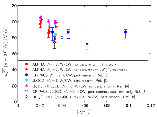
Figure 2: Summary of the strange quark mass data from lattice simulations. In the legend the discretizations used are indicated in the form gauge action/fermion action. The dictionary reads: W: Wilson gauge action; I: Iwasaki gauge action; LW: 1–loop tadpole improved Lüscher–Weisz gauge action; CW: Wilson–clover fermion action; KS: Asqtad staggered fermion action. The dotted lines represent the quenched result [14]. $r_{0}=0.5$ fm has been used for all the datasets, whereas in [1] $r_{0}=0.467$ fm was used for the data from [4], as suggested thereby.

We give our conclusions discussing the collection of results in figure 2. By comparing different O($a$) improved regularizations we see that cutoff effects on the strange quark mass at a lattice spacing of $0.1$ fm are around 20%. It is more difficult to assess the $N_{\rm f}$ dependence mainly because only perturbative renormalization has been used in the 3-flavor case. On the other hand the comparison of $N_{\rm f}=2$ determinations indicates that the use of perturbation theory for the renormalization constants underestimates the quark mass.

Acknowledgement. We thank NIC/DESY for allocating computer time on the APEmille machines and the APE group for their support. This work has been supported by the SFB Transregio 9 and by the Deutsche Forschungsgemeinschaft in the Graduiertenkolleg GK 271 as well as by the European Community’s Human Potential Programme under contract HPRN-CT-2000-00145.

References

- [1] ALPHA, M. Della Morte et al., to appear in Nucl. Phys. B, hep-lat/0507035.
- [2] CP-PACS, A. Ali Khan et al., Phys. Rev. D65 (2002) 054505, hep-lat/0105015.
- [3] JLQCD, S. Aoki et al., Phys. Rev. D68 (2003) 054502, hep-lat/0212039.
- [4] QCDSF, M. Göckeler et al., (2004), hep-ph/0409312, and these proceedings.
- [5] CP-PACS, T. Ishikawa et al., Nucl. Phys. Proc. Suppl. 140 (2005) 225, hep-lat/0409124.
-
[6]
HPQCD, C. Aubin et al.,
Phys. Rev. D70 (2004) 031504, hep-lat/0405022;
Q. Mason, these proceedings. - [7] H. Leutwyler, Phys. Lett. B378 (1996) 313, hep-ph/9602366.
-
[8]
K. Jansen and R. Sommer, Nucl. Phys. B530 (1998) 185,
Erratum-ibid. B643 (2002) 517;
CPPACS/JLQCD, N. Yamada et al. Phys. Rev. D71 (2005) 054505, hep-lat/0406028. - [9] ALPHA, M. Della Morte, R. Hoffmann and R. Sommer, JHEP 03 (2005) 029, hep-lat/0503003.
- [10] S. Sint, Nucl. Phys. B421 (1994) 135, hep-lat/9312079.
- [11] ALPHA, S. Capitani et al. Nucl. Phys. B544 (1999) 669, hep-lat/9810063.
-
[12]
ALPHA, M. Della Morte et al., JHEP 07 (2005) 007, hep-lat/0505026;
R. Hoffmann et al., these proceedings, PoS (LAT2005) 232. - [13] ALPHA, M. Della Morte et al., Nucl. Phys. B713 (2005) 378, hep-lat/0411025.
- [14] ALPHA/UKQCD, J. Garden, J. Heitger, R. Sommer and H. Wittig, Nucl. Phys. B571 (2000) 237, hep-lat/9906013.
- [15] R. Sommer, Nucl. Phys. B411 (1994) 839, hep-lat/9310022.
- [16] ALPHA/CPPACS/JLQCD, R. Sommer et al., Nucl. Phys. Proc. Suppl. 129 (2004) 405, hep-lat/0309171.
- [17] J. Gasser and H. Leutwyler, Nucl. Phys. B250 (1985) 465.
-
[18]
T. van Ritbergen, J.A.M. Vermaseren and S.A. Larin,
Phys. Lett. B400 (1997) 379, hep-ph/9701390 ;
K.G. Chetyrkin, Phys. Lett. B404 (1997) 161, hep-ph/9703278;
J.A.M. Vermaseren, S.A. Larin and T. van Ritbergen, Phys. Lett. B405 (1997) 327, hep-ph/9703284;
M. Czakon, Nucl. Phys. B710 (2005) 485, hep-ph/0411261.