Gauge theories on a five-dimensional orbifold

Abstract:

We present a construction of non–Abelian gauge theories on the $\mathbb{R}^{4}\times S^{1}/\mathbb{Z}_{2}$ orbifold. We show that no divergent boundary mass term for the Higgs field, identified with some of the fifth dimensional components of the gauge field, is generated. The formulation of the theories on the lattice requires only Dirichlet boundary conditions that specify the breaking of the gauge group. The first simulations in order to resolve the issue whether these theories can be used at low energy as weakly interacting effective theories have been performed. In case of a positive answer, these theories could provide us with a new framework for studying electroweak symmetry breaking.

PoS(LAT2005)280

1 Five–dimensional $SU(N)$ gauge theories

The motivation to look at gauge theories in four plus one compact extra dimensions come from an alternative mechanism for electroweak symmetry breaking where the Higgs field is identified with (some of) the fifth dimensional components of the gauge field. Due to the dimensionful coupling $g_{0}^{\prime}$, five–dimensional gauge theories are nonrenormalizable. Nevertheless they can be employed as effective theories at finite cutoff $\Lambda$. The claim is that the mass of the Higgs field is finite to all orders in perturbation theory. So far phenomenological applications of these ideas are mostly based on 1–loop computations and we would like to understand if they are viable beyond that.

2 A geometrical construction of the $S^{1}/\mathbb{Z}_{2}$ orbifold

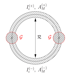
Figure 1: Geometrical construction of the orbifold for gauge fields.

We consider the Euclidean manifold $\mathbb{R}^{4}\times S^{1}$ parameterized by the coordinates $z=(x_{\mu},x_{5})$, where $\mu=0,1,2,3$ and $x_{5}\in(-\pi R,\pi R]$. The coordinates $x_{5}$ are identified modulo $2\pi R$. The definition of gauge fields on such manifold requires (at least) two open overlapping charts. We choose $I_{\epsilon}^{(+)}=\{x_{\mu},x_{5}\in(-\epsilon,\pi R+\epsilon)\}$ and $I_{\epsilon}^{(-)}=\{x_{\mu},x_{5}\in(-\pi R-\epsilon,\epsilon)\}$ and denote by $A_{M}^{(+)}$ and $A_{M}^{(-)}$ ($M=0,1,2,3,5$ is the five–dimensional Euclidean index) the corresponding gauge fields in the Lie algebra. The parameter $\epsilon$ determines the size of the overlaps among the charts $O_{1}\,=\,\{x_{\mu},x_{5}\in(-\epsilon,\epsilon)\}$ and $O_{2}\,=\,\{x_{\mu},x_{5}\in(\pi R-\epsilon,\pi R+\epsilon)\}$. The situation is schematically represented in Fig. 1. In order to ensure gauge invariance, the two gauge fields on the overlaps, where they are both defined, are related by a transition function $\mathcal{G}(z)\in SU(N)$

$$A_{M}^{(-)} = {\cal G}A_{M}^{(+)}{\cal G}^{-1}+{\cal G}\partial_{M}{\cal G}^{-1}\,,\quad\mbox{on $O_{i}$, $i=1,2$}\,.$$ (1)

The orbifold projection of $S^{1}$ onto $S^{1}/\mathbb{Z}_{2}$ amounts to the identification of points and fields under the $\mathbb{Z}_{2}$ reflection $\mathcal{R}$, which is defined to act on coordinates and fields through

$$\mathcal{R}\,z = {\bar{z}}\,,\qquad{\bar{z}}=(x_{\mu},-x_{5})\,,$$ (2)

$$\mathcal{R}\,A_{M}(z) = \alpha_{M}A_{M}({\bar{z}})\,,\qquad\alpha_{\mu}=1\,,\quad\alpha_{5}=-1\,.$$ (3)

The orbifold projection for the gauge field identifies

$$\mathcal{R}\,A_{M}^{(+)} \equiv A_{M}^{(-)}$$ (4)

on the overlaps, where $\mathcal{R}\,A_{M}^{(+)}$ is defined. Outside the overlaps the fields $A_{M}^{(+)}(z)$ and $A_{M}^{(-)}({\bar{z}})$ are identified. At this point we need only one gauge field, which we take to be $A_{M}\equiv A_{M}^{(+)}$. Eq. (4) together with Eq. (1) imply the constraint

$${\cal R}\,A_{M} = {\cal G}\,A_{M}\,{\cal G}^{-1}+{\cal G}\,\partial_{M}{\cal G}^{-1}\,,$$ (5)

which is self–consistent when

$$(\mathcal{R}\,\mathcal{G})\,\mathcal{G} = \exp(i2\pi k/N)\times\,\mathbf{1}_{N}\,,\quad k=0,1,\ldots,N-1\,.$$ (6)

Covariance of the constraint Eq. (5) requires under a gauge transformation $\Omega$

$${\cal G} \stackrel{{\scriptstyle\Omega}}{{\longrightarrow}} ({\cal R}\,\Omega)\,{\cal G}\,\Omega^{-1}\,.$$ (7)

The gauge covariant derivative of $\mathcal{G}$ is then defined through

$$D_{M}{\cal G} = \partial_{M}{\cal G}+({\cal R}\,A_{M})\,{\cal G}-{\cal G}\,A_{M}\;\equiv\;0$$ (8)

and by virtue of the constraint Eq. (5) it vanishes identically.

The fundamental domain of the orbifold is the strip $I_{0}=\{x_{\mu},x_{5}\in[0,\pi R]\}$. The gauge theory on $I_{0}$ is obtained by starting from the gauge invariant theory formulated on the chart $I_{\epsilon}\equiv I_{\epsilon}^{(+)}=\{x_{\mu},x_{5}\in(-\epsilon,\pi R+\epsilon)\}$ in terms of the gauge field $A_{M}$ and the spurion field (the transition function) $\mathcal{G}$. This theory is gauge invariant under gauge transformations that obey

$$\mathcal{R}\,\Omega = \Omega\,.$$ (9)

The spurion field transforms like the field strength tensor, see Eq. (7). The parameter $\epsilon$ is then set to zero and the spurion field subject to the boundary conditions

$${\cal G}(x_{\mu},x_{5}=0)\,= g =\,{\cal G}(x_{\mu},x_{5}=\pi R)\,,$$ (10)

where $g$ is a constant matrix. It follows from Eq. (6) that $g^{2}$ is an element of the center of $SU(N)$. At the boundaries $x_{5}=0$ and $x_{5}=\pi R$ of the strip all derivatives of $\mathcal{G}$ are required to vanish. From Eq. (5) the boundary conditions for any field can be derived, for example

$$\alpha_{M}\,A_{M}\,=\,g\,A_{M}\,g^{-1} \mbox{Dirichlet boundary conditions}\,,$$ (11)

$$-\alpha_{M}\,\partial_{5}A_{M}\,=\,g\,\partial_{5}A_{M}\,g^{-1} \mbox{Neumann boundary conditions}\,.$$ (12)

It is clear from Eq. (7) that only the gauge transformations satisfying

$$[g,\Omega(z)] = 0\,,\quad{\rm at}\;x_{5}=0\;{\rm and}\;x_{5}=\pi R$$ (13)

are still a symmetry: the gauge group is broken at the boundaries if $g\neq 1$.

A parameterization of the matrix $g$ is given by

$$g = {\rm e}^{-2\pi iV\cdot H}$$ (14)

where $H=\{H_{i}\}$, $i=1,\ldots,N-1$ are the Hermitian generators of the Cartan subalgebra of $SU(N)$ and $V=\{V_{i}\}$ is the twist vector of the orbifold. It follows that under group conjugation by $g$ the Hermitian generators $T^{A}$ of $SU(N)$ transform as $g\,T^{A}\,g^{-1}=\eta^{A}\,T^{A}$, $\eta^{A}=\pm 1$ [1]. The breaking of the gauge group in Eq. (13) is determined by the choice of the twist vector and is of the form

$$SU(p+q) \longrightarrow \mathcal{H}=SU(p)\times SU(q)\times U(1)\,.$$ (15)

Eq. (11) means that only the components $A_{5}^{A}$ associated with generators $T^{A}$, which do not commute with $g$ survive at the orbifold boundaries. Therefore we identify $[A_{5}(z),g]$ with the Higgs field. It transforms in some representation of $\mathcal{H}$.

It is plausible that we can apply the Symanzik analysis of counterterms for renormalizable field theories with boundaries [2, 3] to the nonrenormalizable orbifold theory defined on the strip $I_{0}$. The latter is considered as effective theory at finite cutoff $\Lambda$. The boundary term

$${\rm{\rm tr}}\,\{[A_{5},g][A_{5},g]\}$$ (16)

is a Higgs mass term and is invariant under gauge transformations of the unbroken subgroup $\mathcal{H}$. It would be a quadratically divergent (with the cutoff $\Lambda$) boundary mass term. Explicit 1–loop calculations [4] indicate that this term is not present and a shift symmetry argument forbids it [5].

In our geometrical construction the term Eq. (16) has to be derived from a gauge invariant term in the theory formulated on the chart $I_{\epsilon}$. It could come from

$${\rm tr}\,\{D_{5}{\cal G}\,D_{5}{\cal G}\} \equiv 0$$ (17)

but this term vanishes identically due to Eq. (8). In fact there are no boundary terms of dimension less than or equal to four. The lowest dimensional boundary terms are the dimension five terms

$$\frac{1}{{g_{0}^{\prime}}^{2}}\,{\rm Re}\,{\rm tr}\,\{g\,F_{MN}\,F_{MN}\} \frac{1}{{g_{0}^{\prime}}^{2}}\,{\rm Re}\,{\rm tr}\,\{g\,F_{MN}\,g\,F_{MN}\}\,.$$ and (18)

3 Lattice simulations of $SU(2)$

On the lattice we define the orbifold theory in the strip $I_{0}=\{z=a(n_{\mu},n_{5})|\;0\leq n_{5}\leq N_{5}=\frac{\pi R}{a}\}$, where $a$ is the lattice spacing. In the following we assume periodic boundary conditions in the directions $\mu=0,1,2,3$. The Wilson action for the orbifold reads

$$S^{\rm orb}_{\rm W}[U]\,=\,\frac{\beta}{2N}\sum_{p}w(p)\,{\rm tr}\{1-U(p)\}\,,\quad w(p)\,=\,\left\{\begin{array}[]{ll}\frac{1}{2}&\mbox{$p$ in the boundary}\\ 1&\mbox{in all other cases.}\end{array}\right.$$ (21)

where the sum is over oriented plaquettes $p$. The bare dimensionful gauge coupling $g_{0}^{\prime}$ on the lattice is defined through $\beta=2Na/{g_{0}^{\prime}}^{2}$. The action Eq. (21) is identical to the one for the Schrödinger Functional (SF) [6].

As it was shown in Ref. [1], on the lattice the orbifold is specified by imposing the following Dirichlet boundary conditions in the four–dimensional boundary planes of the strip $I_{0}$

$$U(z,\mu) = g\,U(z,\mu)\,g^{-1}\,,\quad\mbox{at $n_{5}=0$ and $n_{5}=N_{5}$}\,.$$ (22)

We emphasize that these boundary conditions are of a different type than for the SF, as they constrain the gauge variables at the boundaries but do not fix them completely. In the naive continuum limit the Dirichlet and Neumann boundary conditions, the latter “carried” by the gluon propagator, are recovered [1].

We present here first results from simulations of the five–dimensional $SU(2)$ gauge theory on the orbifold. The matrix $g$ in Eq. (14) is given by $g=-i\sigma_{3}$ ($V=1/2$) and Eq. (22) implies that the boundary links are parameterized in terms of a $U(1)$ phase $\phi(z,\mu)$

$$U(z,\mu) = \exp(i\phi(z,\mu)\sigma_{3})\,,\quad\mbox{at $n_{5}=0$ and $n_{5}=N_{5}$}\,.$$ (23)

The simulation algorithm is composed of heatbath and overrelaxation updates in the bulk, where the gauge group is $SU(2)$, and for the four–dimensional $U(1)$ boundary links.

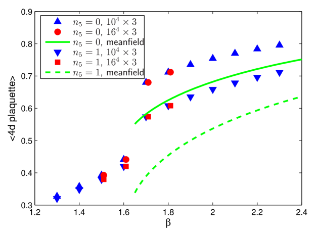
Figure 2: Orbifold boundaries and bulk.

Five–dimensional $SU(N)$ gauge theories in infinite volume have a phase transition separating the Coulomb phase with massless gluons at very large $\beta$ from the confining phase at very small $\beta$ [7, 8]. For $SU(2)$ the phase transition is at $\beta_{c}=1.642(15)$ [7]. In Fig. 2 we show results of simulations of the orbifold with $N_{5}=3$ and two different four–dimensional volumes $10^{4}$ and $16^{4}$. We plot the expectation values of the four–dimensional plaquettes at $n_{5}=0$ and $n_{5}=1$ (equal to the ones at $n_{5}=3$ and $n_{5}=2$ respectively). We see that the orbifold is similar to the torus geometry in the sense that around $\beta=1.6$ there is a jump of plaquette values and we observed hysteresis effects. In the middle of the extra dimension the plaquette values are very close to the ones on a $10^{4}\times 4$ torus. At the boundaries the plaquettes are “colder”. We do not observe significant effects when changing the four–dimensional volume.

We have done a meanfield computation for the orbifold geometry as follows. We set

$$U(z,\mu) = u(n_{5})\,\times\,\mathbf{1}_{2}\,,\qquad\qquad\quad n_{5}\,=\,0,\ldots,N_{5}$$ (24)

$$U(z,5) = u(n_{5}+1/2)\,\times\,\mathbf{1}_{2}\,,\qquad n_{5}\,=\,0,\ldots,N_{5}-1$$ (25)

The meanfield computation amounts to an iterative solution of a system of equations for the factors $u$. Each link is equated to its expectation value in the fixed configuration of all the other links for a given value of $\beta$. We get, for the boundary links at $n_{5}=0$ (plus sign) and $n_{5}=N_{5}$ (minus sign):

$$b = \beta[(1/2)\,6\,u(n_{5})^{3}+u(n_{5}\pm 1)\,u(n_{5}\pm 1/2)^{2}]$$ (26)

$$u(n_{5}) = I_{1}(b)/I_{0}(b)\,,$$ (27)

for the $SU(2)$–links $U(z,\mu)$ in the bulk at $n_{5}=1,\ldots,(N_{5}-1)$:

$$b = \beta[6\,u(n_{5})^{3}+u(n_{5}+1/2)^{2}\,u(n_{5}+1)+u(n_{5}-1/2)^{2}\,u(n_{5}-1)]$$ (28)

$$u(n_{5}) = I_{2}(b)/I_{1}(b)\,,$$ (29)

and for the $SU(2)$–links $U(z,5)$ along the extra dimension at $n_{5}=(1/2)\ldots(N_{5}-1/2)$

$$b = \beta\,8\,u(n_{5}-1/2)\,u(n_{5})\,u(n_{5}+1/2)$$ (30)

$$u(n_{5}) = I_{2}(b)/I_{1}(b)\,.$$ (31)

The meanfield plaquette values $u(0)^{4}$ and $u(1)^{4}$ for $N_{5}=3$ are plotted in Fig. 2 for “large” $\beta$ values (at lower $\beta$ only the solution $u=0$ is found). They show qualitatively the difference between plaquettes at the boundaries and in the middle of the extra dimension as it is seen in the simulations.

References

- [1] N. Irges and F. Knechtli, Nonperturbative definition of five–dimensional gauge theories on the orbifold, Nucl. Phys. B719 (2005) 121, [hep-lat/0411018].
- [2] K. Symanzik, Schrödinger representation and Casimir effect in renormalizable quantum field theory, Nucl. Phys. B190 (1981) 1.
- [3] M. Lüscher, Schrödinger representation in quantum field theory, Nucl. Phys. B254 (1985) 52.
- [4] G. von Gersdorff, N. Irges and M. Quiros, Bulk and brane radiative effects in gauge theories on orbifolds, Nucl. Phys. B635 (2002) 127, [hep-th/0204223].
- [5] G. von Gersdorff, N. Irges and M. Quiros, Radiative brane–mass terms in orbifold gauge theories, Phys. Lett. B551 (2003) 351, [hep-ph/0210134].
- [6] M. Lüscher, R. Narayanan, P. Weisz and U. Wolff, The Schrödinger Functional: a renormalizable probe for non–Abelian gauge theories, Nucl. Phys. B384 (1992) 168, [hep-lat/9207009].
- [7] M. Creutz, Confinement and the critical dimensionality of space–time, Phys. Rev. Lett. 43 (1979) 553.
- [8] B.B. Beard, R.C. Brower, S. Chandrasekharan, D. Chen, A. Tsapalis and U.-J. Wiese, D–theory: field theory via dimensional reduction of discrete variables, Nucl. Phys. B(Proc. Suppl.)63 (1998) 775, [hep-lat/9709120].