Baryon magnetic moments in the background field method

Abstract

We present a calculation of the magnetic moments for the baryon octet and decuplet using the background-field method and standard Wilson gauge and fermion actions in the quenched approximation of lattice QCD. Progressively smaller static magnetic fields are introduced on a $24^{4}$ lattice at beta=6.0 and the pion mass is probed down to about 500 MeV. Magnetic moments are extracted from the linear response of the masses to the background field.

1 Introduction

Magnetic moments are an important fundamental property of particles. They determine dynamical response of a bound system to a soft external stimulus, and provide valuable insight into internal strong interaction structure. Efforts to compute the magnetic moment on the lattice can be divided into two categories. One is from form factors which involves three-point functions [1, 2, 3, 4, 5, 6, 7]. The other is the background field method using only two-point functions [8, 9, 10, 11]. The form factor method requires an extrapolation to $G_{M}(Q^{2}=0)$ that is potentially fallible due to the discrete momentum on the lattice [12]. The background field method, on the other hand, is free from this problem since a static magnetic field is applied to the gauge background. Here we report a calculation in this method. It is an extension of our work on electric and magnetic polarizabilities [13, 14, 15].

2 Method

In order to place a magnetic field on the lattice, we construct an analogy to the continuum case. The fermion action is modified by the minimal coupling prescription

$$D_{\mu}=\partial_{\mu}+gG_{\mu}+qA_{\mu}$$ (1)

where $q$ is the charge of the fermion field and $A_{\mu}$ is the vector potential describing the background field. On the lattice, the prescription amounts to a modified link variable

$$U_{\mu}^{\prime}=U_{\mu}U_{\mu}^{(B)}.$$ (2)

Choosing $A_{y}=Bx$, a constant magnetic field B can be introduced in the $z$-direction. Then the phase factor is in the y-links

$$U_{y}^{(B)}=\exp{(iqa^{2}Bx)}.$$ (3)

On a finite lattice with periodic boundary conditions, to get a constant magnetic field, B has to be quantized by the condition

$$qBa^{2}={2\pi n\over N_{x}},\hskip 2.84526ptn=1,2,3,\cdots$$ (4)

to ensure that the magnetic phase factor is periodic in the x-direction. However, for $N_{x}=N_{y}=16$ and $1/a=2GeV$, the lowest field would give the proton a mass shift of about 390 MeV, which is too large (the proton is severely distorted). In this work, we abandon the quantization condition and choose to work with smaller fields. To minimize the boundary effects, we work with fixed (or Dirichlet) b.c. in the x-direction and large $N_{x}$, so that quarks originating in the middle of the lattice have little chance of propagating to the edge.

We use $24^{4}$ lattice at $\beta=6.0$, and six kappa values $\kappa$=0.1515, 0.1525, 0.1535, 0.1540, 0.1545, 0.1555, corresponding to pion mass of 1015, 908, 794, 732, 667, 522 MeV. The critical value of kappa is $\kappa_{c}$=0.1571. The strange quark mass is set at $\kappa$=0.1535. The source location for the quark propagators is (x,y,z,t)=(12,1,1,2). We analyzed 87 configurations. The following five dimensionless numbers $\eta=qBa^{2}$=+0.00036, -0.00072, +0.00144, -0.00288, +0.00576 give four small B fields (two positive, two negative) at $eBa^{2}$=-0.00108, +0.00216, -0.00432, +0.00864 for both u and d (or s) quarks. Note that ”small” here is in the sense that the mass shift is only a fraction of the proton mass: $\mu B/m\sim$ 1 to 5% at the smallest pion mass. In absolute terms, the field is enormous: $B\sim 10^{13}$ tesla.

The mass shift in the presence of small fields can be expanded as a polynomial in B,

$$\delta m(B)=m(B)-m(0)=c_{1}B+c_{2}B^{2}+c_{3}B^{3}+c_{4}B^{4}+\cdots$$ (5)

To eliminate the contamination from the even-power terms, we calculate mass shifts both in the field $B$ and its reverse $-B$ for each value of $B$, then take the difference and divide by 2. So in terms of cost, our calculation is equivalent to 11 separate spectrum calculations: 5 original $\eta$ values, 5 reversed, plus the one at zero field to set the baseline. In light of future dynamical simulations, the factor can be reduced to 3 if only one nonzero field is desired. Another benefit of repeating the calculation with the field reversed is that by taking the average of $\delta m(B)$ and $\delta m(-B)$ in the same dataset, one can eliminate the odd-powered terms in the mass shift. The coefficient of the leading quadratic term is directly related to the so-called magnetic dipole polarizability ($\beta$).

For a Dirac particle of spin $s$ in uniform fields,

$$E_{\pm}=m_{\pm}\pm\mu B$$ (6)

where the upper sign means spin up and the lower sign means spin-down, and $\mu=g{e\over 2m}s$. In our data, $m_{+}$ and $m_{-}$ correspond to the ‘11’ and ‘22’ diagonal components of the baryon correlation function in the absence of the background field. They are the same within statistical fluctuations. The average of the two components is usually used to extract the proton mass. We tried the following three methods to extract the g factors, and found they are equivalent within statistical errors.

$$g=\left({2m_{+}m_{-}\over m_{+}+m_{-}}\right){(E_{+}-m_{+})-(E_{-}-m_{-})\over eBs}$$ (7)

$$g={m_{+}(E_{+}-m_{+})-m_{-}(E_{-}-m_{-})\over eBs}$$ (8)

$$g={(E_{+}^{2}-m_{+}^{2})-(E_{-}^{2}-m_{-}^{2})\over 2eBs}$$ (9)

The results quoted are from Eq. (7).

3 Results and discussion

Fig. 1 displays a typical effective mass plot at the six kappa values for the strongest magnetic field for the proton. Good plateaus exist for all six quark masses. Our results are extracted from the time window 12 to 15. Fig. 2 displays a typical mass shift, defined as $\delta=g(eBs)$ from Eq. (7), as a function of the field for the proton. There is good linear behavior going through the origin for all the fields when the quark mass is heavy, an indication that contamination from the higher terms has been effectively eliminated. This is also confirmed numerically by the smallness of the coefficient in the $B^{3}$ term as shown in the same figure. At the lightest quark mass (lower right corner), there is a slight deviation from linear behavior. For this reason, we only use the two smallest field values to do the linear fit at all the quark masses.

Fig. 3 shows the results for the proton and the neutron as a function of pion mass squared . Note that the g factors directly extracted from the data are in the particles natural magnetons. To convert them to the commonly-used nuclear magnetons ($\mu_{N}$), we have scaled the results by the factor $938/M$ where $M$ is the mass of the particle measured in the same calculation at each quark mass. The line is a simple chiral fit using the ansatz

$$\mu=a_{0}+a_{1}m_{\pi}.$$ (10)

There is a lot of effort in the literature on magnetic moments and their chiral extrapolations based on effective field theories [17, 18, 19, 20, 21, 22, 23, 24]. Although different approaches produce the same chiral behavior near the chiral limit, there are issues surrounding the range of validity and model-independence away from the chiral limit. The lowest pion mass in our results (around 500 MeV) is probably too large for a meaningful application of the results from these studies. Our goal here is to present the lattice data. The simple ansatz in Eq. (10) serves only to show that there is onset of non-analytic behavior as pion mass is lowered, so a linear extrapolation is probably not a good idea. To get some idea about the systematic uncertainty in the chiral fit, we tried two other different forms, one is

$$\mu=a_{0}+a_{1}m_{\pi}+a_{2}m_{\pi}^{2}$$ (11)

and the other the Pade form [24]

$$\mu=a_{0}/(1+a_{1}m_{\pi}+a_{2}m_{\pi}^{2}).$$ (12)

The extrapolated value to the physical point is 3.04(6) for the proton and -1.84(3) for the neutron from Eq. (10), 3.78(5) and -2.03(2) from Eq. (11), and 4.21(5) and -1.84(2) from Eq. (12).

Fig. 4 shows the results in the octet sigma channel. The perfect agreement for the $\Sigma^{-}$ should be taken as a coincidence. Fig. 5 shows the results for the four delta states. The agreement with the well-known $\Omega^{-}$ moment in Fig. 5 is particularly encouraging since no adjustment is needed for this point (it is a direct comparison with the experimental value). We take it as a sign of the correctness of our calculation. The experimental numbers in the delta channel are not well-established. The experimental value for $\Delta^{+}$ (slightly shifted for better view) is taken from Ref. [25]. For reader’s convenience, all of our results are summarized in Table 1. Finally, Fig. 6 shows the proton and $\Delta^{+}$ together. The opposite curvatures are a signature of quenched chiral physics. A similar behavior has been observed by  [26, 27] using the form factor method.

About the issue of finite-volume effects as related to the Dirichlet boundary conditions, we did some further study. We repeated the entire calculation on a smaller lattice $16^{3}\times 24$, while keeping all the paraemeters the same as on the larger lattice $24^{3}\times 24$. So the only difference is the spatial box size ($16^{3}$ vs. $24^{3}$). Assuming the lattice spacing is the same (a=0.1 fm) on the two lattices, the dimentionless combination $m_{\pi}L_{x}$ for the lightest pion is about 6.2 on the $24^{3}\times 24$, and 4.2 on the $16^{3}\times 24$. The effects on the magnetic moments of the proton and neutron are shown in Fig. 7. Relatively significant finite-volume effects are revealed, even at the heavier pion masses, ’spoiling’ the trend towards the physical point. We take this as indication that the $16^{3}\times 24$ lattice is too small. To really pin down the finite-volume effects, we should repeat the calculation on a larger lattice, say $32^{3}\times 32$. But it is currently beyond our computing resources.

4 Conclusion

In conclusion, we have computed the magnetic moments of the baryon octet and decuplet on the lattice using the background field method and standard lattice technology. Overall, our results are consistent with experimental observations. Detailed comparison with experiment must await a full account of systematic errors present in the results, such as finite-volume effects. In addition, there is a need to push the calculations to smaller pion masses so that reliable chiral extrapolations can be applied. Nonetheless, our results demonstrate that the method is robust and relatively cheap, as compared to the form factor method. Only mass shifts are required. This may facilitate the push to smaller pion masses, perhaps with the help of chiral fermions (overlap, domain-wall, twisted mass, …). Finally, we foresee no technical problems in doing dynamical (full-QCD) background-field calculations in order to remove the effects of the quenched approximation.

This work is supported in part by U.S. Department of Energy under grant DE-FG02-95ER40907, and by NSF grant 0070836. The computing resources at NERSC and JLab have been used.

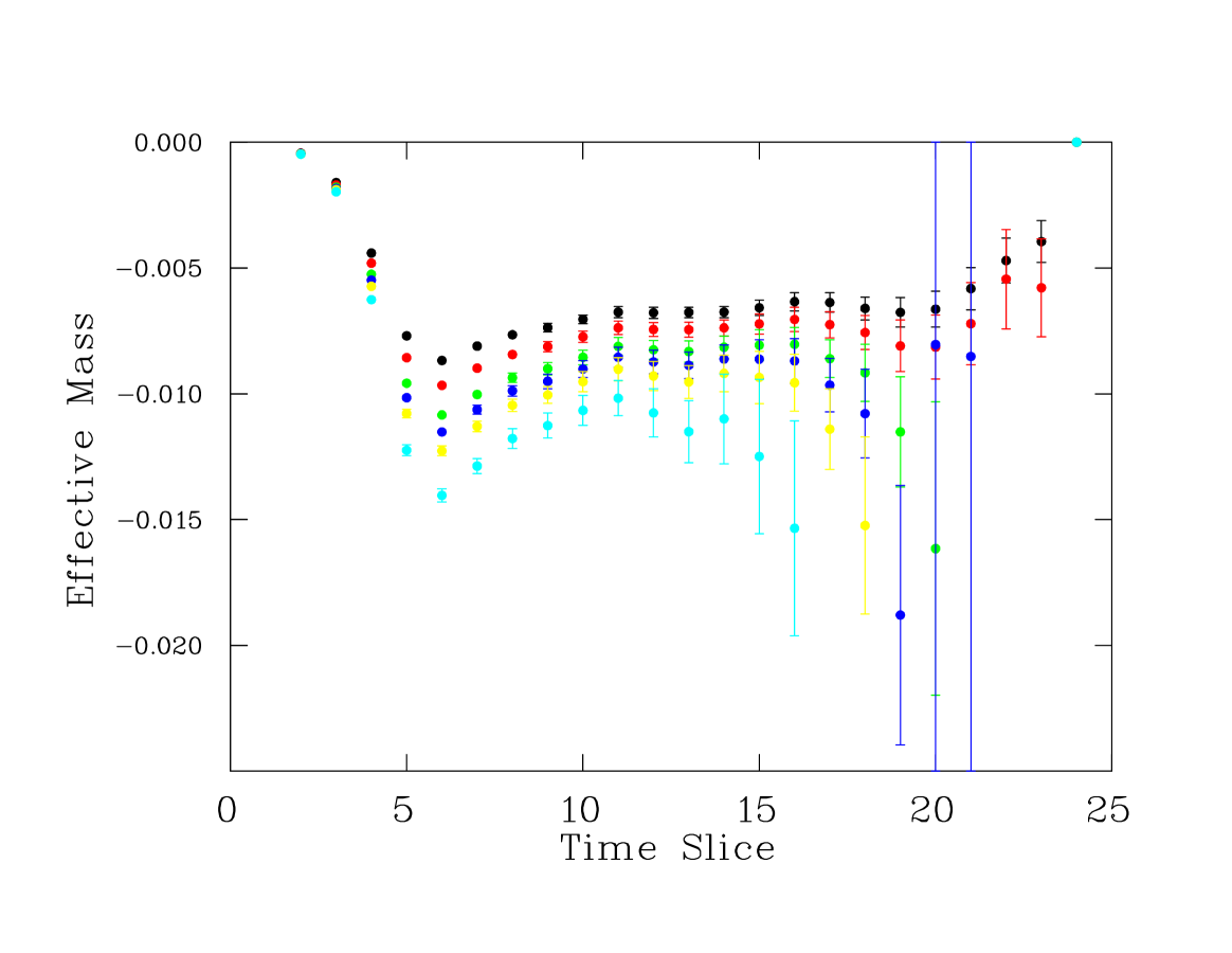
Figure 1: Effective mass plot for proton mass shifts as the strongest magnetic field in lattice units. Plotted is the combination $(E_{+}-m_{+})-(E_{-}-m_{-})$ in Eq. (7) at all six quark masses in the order of decreasing quark mass from top to bottom.

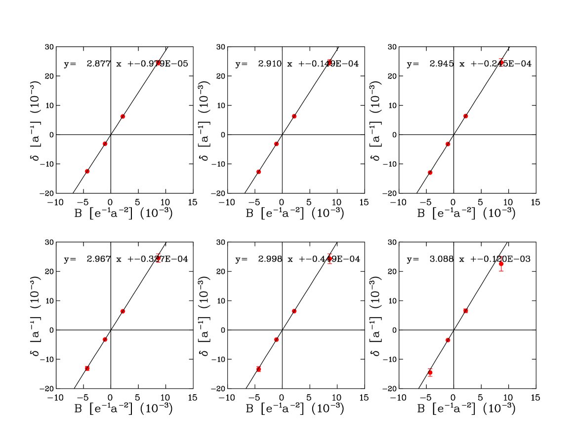
Figure 2: Proton mass shifts as a function of magnetic field $B$ in lattice units at the six quark masses (lightest in the lower right corner). The slope of the mass shift at each quark mass gives the g factor corresponding to that quark mass. The line is a fit using only the two smallest B values.

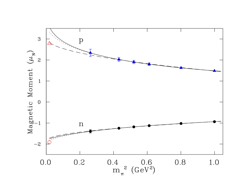
Figure 3: Magnetic moments (in nuclear magnetons) for the proton and neutron as a function of $m_{\pi}^{2}$. The 3 lines are chiral fits according to Eq. (10) (dashed), Eq. (11) (dotted), and Eq. (12) (solid). The experimental values, taken from the PDG [16], are indicated by the empty symbols.

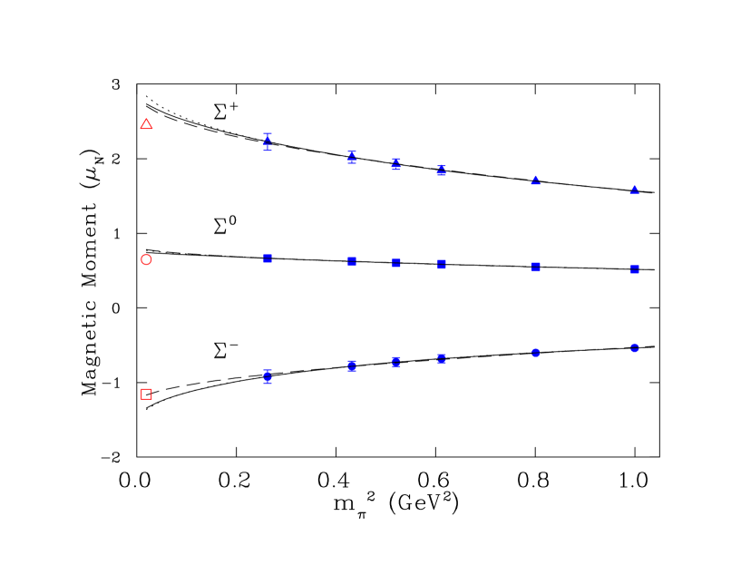
Figure 4: Magnetic moments for the octet $\Sigma$.

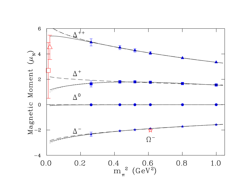
Figure 5: Magnetic moments for the $\Delta$ states.

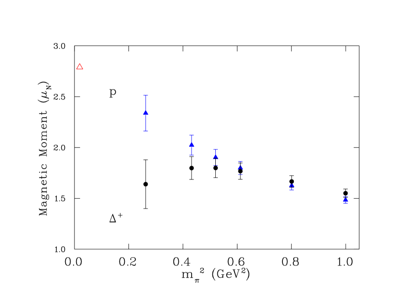
Figure 6: Comparison of magnetic moments of the proton and $\Delta^{+}$.

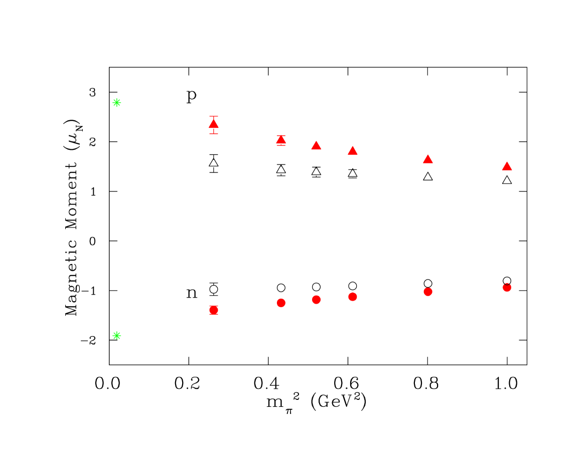
Figure 7: Finite-volume effects on the magnetic moments of the proton and neutron. The solid (red) symbols are from the $24^{3}\times 24$ lattice, and the empty symbols are from the $16^{3}\times 24$ lattice. The experimental values are denoted by the stars.

Table 1: The computed magnetic moments for the baryon octet and decuplet in nuclear magnetons ($\mu_{N}$) as a function of the pion mass. The extrapolated values are based on Eq (10). The experimental values are taken from the PDG [16].

$\kappa$	0.1515	0.1525	0.1535	0.1540	0.1545	0.1555	Extrap.	Expt.
$m_{\pi}$ (GeV)	1.015	0.908	0.794	0.732	0.667	0.522
p	1.48(3)	1.63(4)	1.80(6)	1.90(8)	2.02(10)	2.34(17)	3.04(6)	2.79
n	-0.94(2)	-1.02(2)	-1.13(3)	-1.18(4)	-1.25(5)	-1.39(8)	-1.84(3)	-1.91
$\Sigma^{+}$	1.57(4)	1.70(5)	1.85(6)	1.93(7)	2.02(8)	2.23(11)	2.87(3)	2.45
$\Sigma^{0}$	0.52(1)	0.55(1)	0.59(2)	0.61(2)	0.63(2)	0.67(3)	0.76(1)	0.65
$\Sigma^{-}$	-0.54(4)	-0.60(4)	-0.68(6)	-0.73(6)	-0.78(7)	-0.92(9)	-1.48(5)	-1.16
$\Xi^{0}$	-1.07(4)	-1.10(4)	-1.13(4)	-1.15(4)	-1.17(5)	-1.21(7)	-1.37(1)	-1.25
$\Xi^{-}$	-0.76(6)	-0.77(7)	-0.77(8)	-0.77(8)	-0.77(9)	-0.78(11)	-0.82(1)	-0.65
$\Lambda$	-0.59(2)	-0.60(2)	-0.60(2)	-0.61(2)	-0.61(2)	-0.62(3)	-0.70(1)	-0.61
$\Delta^{++}$	3.35(7)	3.68(9)	4.06(12)	4.28(14)	4.50(16)	4.92(28)	5.24(18)	4.52(1.00)
$\Delta^{+}$	1.55(4)	1.67(6)	1.77(8)	1.80(10)	1.80(11)	1.64(24)	0.97(8)
$\Delta^{0}$	-0.002(0)	-0.003(0)	-0.004(1)	-0.005(1)	-0.007(1)	-0.011(6)	-0.035(2)
$\Delta^{-}$	-1.58(4)	-1.73(5)	-1.89(7)	-1.98(8)	-2.07(10)	-2.34(17)	-2.98(19)
$\Sigma*^{+}$	1.40(5)	1.56(6)	1.72(8)	1.80(10)	1.86(11)	1.88(17)	1.27(6)
$\Sigma*^{0}$	-0.13(1)	-0.09(1)	-0.03(0)	-0.01(0)	0.03(0)	0.08(2)	0.33(5)
$\Sigma*^{-}$	-1.68(5)	-1.76(7)	-1.83(9)	-1.87(10)	-1.89(11)	-1.93(16)	-1.88(4)
$\Xi*^{0}$	-0.09(2)	-0.06(1)	-0.022(5)	-0.002(1)	0.018(6)	0.05(3)	0.16(4)
$\Xi*^{-}$	-0.59(7)	-0.61(8)	-0.62(9)	-0.62(10)	-0.63(10)	-0.63(11)	-0.62(1)

References

- [1] G. Martinelli and C.T. Sachrajda, Nucl. Phys. B316, 355 (1989).
- [2] D.B. Leinweber, T. Draper, R.M. Woloshyn, Phys. Rev. D43, 1659 (1991); Phys. Rev. D46, 3067 (1992); Phys. Rev. D48, 2230 (1993).
- [3] W. Wilcox, T. Draper and K.F. Liu, Phys. Rev. D46, 1109 (1992).
- [4] V. Gadiyak, X. Ji, C. Jung, Phys. Rev. D65, 094510 (2002).
- [5] Göckeler et. al., Phys. Rev. D71, 034508 (2005).
- [6] J. Zanotti, Boinepalli, D.B. Leinweber, A.W. Williams, J.B. Zhang, hep-lat/0401029.
- [7] I.C. Cloet, D.B. Leinweber, A.W. Thomas, Phys. Lett. B563, 157 (2003).
- [8] G. Martinelli et. al., Phys. Lett. B116, 434 (1982).
- [9] C. Bernard, T. Draper, K. Olynyk, Phys. Rev. Lett. 49, 1076 (1982); C. Bernard, T. Draper, K. Olynyk, M. Rushton, Nucl. Phys. B220, 508 (1983).
- [10] J. Smit and J.C. Vink, Nucl. Phys. B286, 485 (1987).
- [11] H.R. Rubinstein, S. Solomon and T. Wittlich, Nucl. Phys. B457, 577 (1995).
- [12] W. Wilcox, Phys. Rev. D66, 017502 (2002).
- [13] J. Christensen, W. Wilcox, F.X. Lee, L. Zhou, hep-lat/0408024.
- [14] L. Zhou, F.X. Lee, W. Wilcox, J. Christensen, Nucl. Phys. B (Proc. Suppl.) 119, 272 (2003).
- [15] L. Zhou, PhD dissertation (2004) (unpublished).
- [16] Particle Daata Group, Phys. Lett. B592, 1 (2004).
- [17] B. Borasoy, R. Lewis, A. Ouimet, Phys. Rev. D65, 114023 (2002).
- [18] D. Arndt, B.C. Tiburzi, Phys. Rev. D68, 114503 (2003).
- [19] M.J. Savage, Nucl. Phys. A700, 359 (2002).
- [20] S.R. Beane, M.J. Savage, Phys. Rev. D68, 114502 (2003).
- [21] S.R. Beane, Phys. Rev. D70, 034507 (2004); Nucl. Phys. B695, 192 (2004).
- [22] T.R. Hemmert, M. Procura, W. Weise, Nucl. Phys. A721, 938 (2003).
- [23] R.D. Young, D.B. Leinweber, A.W. Thomas, Phys. Rev. D71, 014001 (2005).
- [24] D.B. Leinweber, Phys. Rev. D69, 014005 (2004).
- [25] M. Kotulla et. al., Phys. Rev. Lett. 89, 272001 (2002).
- [26] J. Zanotti, D.B. Leinweber, A.W. Williams, J.B. Zhang, Nucl. Phys. B (Proc. Suppl.) 129-130, 287 (2004), hep-lat/0309186.
- [27] R.D. Young, D.B. Leinweber, A.W. Thomas, Nucl. Phys. B (Proc. Suppl.) 129-130, 290 (2004), hep-lat/0309187, hep-lat/0311038.