Two-colour Lattice QCD with dynamical fermions at non-zero density versus Matrix Models

Abstract:

We provide first evidence that Matrix Models describe the low lying complex Dirac eigenvalues in a theory with dynamical fermions at non-zero density. Lattice data for gauge group $SU(2)$ with staggered fermions are compared to detailed analytical results from Matrix Models in the corresponding symmetry class, the complex chiral Symplectic Ensemble. They confirm the predicted dependence on chemical potential, quark mass and volume.

PoS(LAT2005)197

1 Introduction

In the past few years many new analytical results have emerged from Matrix Models (MM) for the Dirac operator spectrum with non-vanishing chemical potential $\mu\neq 0$. There are 3 different possible chiral symmetry breaking patterns [1] and in the MM picture they differ crucially in the way the eigenvalues are depleted from the imaginary axis through $\mu\neq 0$ [2]. Today we have detailed predictions for microscopic Dirac spectra in 2 of these symmetry classes, both quenched and unquenched: QCD and the adjoined representation, where the latter is replaced by $SU(2)$ colour in the fundamental when using staggered fermions as we will do. After first approximate results for quenched QCD [3] the exact quenched density was derived in [4] and related to chiral Perturbation Theory in the epsilon regime ($\epsilon\chi$PT). Unquenched partition functions were computed in [5] and related to $\epsilon\chi$PT, and finally fully unquenched Dirac spectra for QCD became available [6, 7]. Results for the adjoint (or $SU(2)$ staggered) class followed very recently [8] and we confront its unquenched predictions including dependence on $\mu$ and quark mass $m$ with Lattice data here.

Not all the above MM results have been compared to the Lattice so far, precisely due to the sign problem in unquenched QCD. Up to now only quenched simulations at $\mu\neq 0$ using staggered fermions have been successfully described: for QCD [9] (see also [10] in these proceedings) and for $SU(2)$ [11], which we will extend here. Previous comparisons [12] were lacking analytic predictions at the time, they could only be done in the bulk of the spectrum [13] for MM without chiral symmetry. Very recently it has been shown at $\mu=0$ that the previous topology-blindness of staggered fermions can be cured by improvement, as reviewed in [14].

In the last years different ways of attacking the sign problem in QCD were developed: multi-parameter reweighting, Taylor-expansion and imaginary $\mu$ (see [15] for a review and references). However, none of these have been applied so far to the region of $\epsilon\chi$PT where a comparison to MM is expected to hold. We purse a different avenue here, choosing an $SU(2)$ gauge theory without sign problem where dynamical simulations can be performed in a standard way [16]. This permits us to extend previous MM comparisons [17, 18] to $\mu\neq 0$. It is of principle interest to test the validity of all MM predictions for complex Dirac spectra on the Lattice including dynamical fermions.

2 Predictions from Matrix Models with $\mu\neq 0$

In this section we briefly introduce the relevant MM used and give its results for the spectral density. For more details and references we refer to [8]. The MM partition function is given by

$${\cal Z}_{N}^{(2N_{f})}(\{m_{f}\};\mu)\equiv\int\!d\Phi d\Psi\exp\left[-N\mbox{Tr}(\Phi^{\dagger}\Phi\ +\ \Psi^{\dagger}\Psi)\right]\prod_{f=1}^{N_{f}}\det\left(\begin{array}[]{cc}m_{f}\mbox{\bf 1}&i\Phi+\mu\Psi\\ i\Phi^{\dagger}+\mu\Psi^{\dagger}&m_{f}\mbox{\bf 1}\end{array}\right)\!,$$ (1)

where 1 is the quaternion unity element. The two rectangular $(N+\nu)\times N$ matrices, $\Phi$ and $\Psi$, contain quaternion real elements and replace the off-diagonal blocks of the Dirac operator, averaged with a Gaussian matrix weight instead of the gauge action. Here we model the $\mu\gamma_{0}$ part with a random matrix of the same symmetry as the kinetic part, assuming it is non-diagonal in matrix space (as in [6] for QCD). If universality holds this choice of basis should not matter, compared to $\Psi$ replaced by unity as [2]. This assertion is true in the QCD symmetry class, see [4, 5] vs. [6, 7]. The size of the Dirac matrix $2N\sim V$ relates to the volume, and we have chosen rectangular matrices to be in the fixed sector of $\nu\geq 0$ zero eigenvalues or topological charge. Because of using unimproved staggered fermions we set $\nu=0$ in our comparison to the data later.

After transforming the linear combinations $i\Phi^{(\dagger)}+\mu\Psi^{(\dagger)}$ to be triangular we can change to complex eigenvalues $z_{k=1,\ldots,N}$ (rotated to lie on the real axis for $\mu=0$). All their spectral correlation functions can be computed using skew orthogonal Laguerre polynomials in the complex plane [8]. In the large-$N$ limit the complex eigenvalues, masses and chemical potential have to be rescaled

$$\sqrt{2}\ Nz\ \equiv\xi,\ \ \sqrt{2}\ Nm\ \equiv\ \eta,\ \ \mbox{and }\ \ \lim_{N\to\infty,\ \mu\to 0}2N\mu^{2}\ \equiv\ \alpha^{2}\ .$$ (2)

This limit is called weakly non-hermitian as $\mu^{2}$ is rescaled with the volume. The same scaling is found in the static part of the chiral Lagrangian [19] dominating at $\epsilon\chi$PT. While the latter contains two parameters, the chiral condensate $\Sigma$ and the decay constant $F_{\pi}$, the MM contains only one, the variance fixed to be $\Sigma=\sqrt{2}$ here. Thus the constant multiplying $\alpha$ is not know and we are left with 1 free fit parameter, in contrast to the parameter-free MM prediction at $\mu=0$.

The unquenched microscopic spectral density, normalised to $\Im m(\xi)\delta^{\prime}(\Im m(\xi))$ for $\alpha\to 0$,

$$\rho_{weak}^{(4)}(\xi;\eta) = \Delta\rho_{weak}^{(4)}(\xi;\eta)\ +\ \frac{1}{32\alpha^{4}}(\xi^{\ast\,2}-\xi^{2})\ |\xi|^{2}\ K_{2\nu}\left(\frac{|\xi|^{2}}{2\alpha^{2}}\right)\exp\left[+\frac{1}{4\alpha^{2}}(\xi^{2}+\xi^{*\,2})\right]$$

$$\times \int_{0}^{1}ds\int_{0}^{1}\frac{dt}{\sqrt{t}}\mbox{e}^{-2s(1+t)\alpha^{2}}\left(J_{2\nu}(2\sqrt{st}\ \xi)J_{2\nu}(2\sqrt{s}\ \xi^{\ast})\ -\ J_{2\nu}(2\sqrt{s}\ \xi)J_{2\nu}(2\sqrt{st}\ \xi^{\ast})\right),$$

splits into the quenched part and a correction term $\Delta\rho_{weak}^{(4)}(\xi;\eta)$ depending on the mass $\eta$:

$$\Delta\rho_{weak}^{(4)}(\xi;\eta)\ =\ \frac{1}{32\alpha^{4}}(\xi^{\ast\,2}-\xi^{2})\ |\xi|^{2}\ K_{2\nu}\left(\frac{|\xi|^{2}}{2\alpha^{2}}\right)\exp\left[+\frac{1}{4\alpha^{2}}(\xi^{2}+\xi^{*\,2})\right]$$ (4)

$$\times\left\{\left(\int_{0}^{1}\!\!ds\int_{0}^{1}dt\sqrt{\frac{s}{t}}\ \mbox{e}^{-2s(1+t)\alpha^{2}}(J_{2\nu}(2\sqrt{st}\ \xi)I_{2\nu+1}(2\sqrt{s}\ \eta)-\sqrt{t}I_{2\nu+1}(2\sqrt{st}\ \eta)J_{2\nu}(2\sqrt{s}\ \xi))\right)\right.$$

$$\times\left.\left(\int_{0}^{1}\!\!ds\int_{0}^{1}\frac{dt}{\sqrt{t}}\ \mbox{e}^{-2s(1+t)\alpha^{2}}(J_{2\nu}(2\sqrt{st}\,\xi^{*})I_{2\nu}(2\sqrt{s}\,\eta)-I_{2\nu}(2\sqrt{st}\,\eta)J_{2\nu}(2\sqrt{s}\,\xi^{*}))\!\!\right)\!-(\xi\leftrightarrow\xi^{*})\!\right\}$$

$$\times\left[\int_{0}^{1}\!\!ds\int_{0}^{1}dt\sqrt{\frac{s}{t}}\ \mbox{e}^{-2s(1+t)\alpha^{2}}\left(\sqrt{t}I_{2\nu+1}(2\sqrt{st}\ \eta)I_{2\nu}(2\sqrt{s}\ \eta)-I_{2\nu}(2\sqrt{st}\ \eta)I_{2\nu+1}(2\sqrt{s}\ \eta)\right)\right]^{-1}\!.$$

We only give the result for $N_{f}=2$ staggered flavours of equal mass here, see [8] for more flavours and higher correlation functions, as well as [17] for matching MM and staggered flavours.

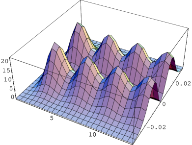
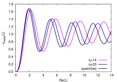
Figure 1: The $N_{f}=2$ flavour spectral density at $\alpha=0.012$ with masses $\eta=8.74$ and $\nu=0$ (left) and a cut through the density normalised to unity for different mass values compared to quenched (right).

Fig. 1 shows this density in the complex plane at weak non-Hermiticity, as we shall compare to data below. The eigenvalues are repelled from the real axis for $\mu\neq 0$, being a distinct feature of this symmetry class (compare to [9] for QCD). We have observed this repulsion in the data for $\mu$ as small as $10^{-6}$. The individual eigenvalues located at the maxima previously are now split into a double peak in the complex plane.

Increasing the mass $\eta\to\infty$ moves the density to the left, bringing it back to the quenched expression, eq. (2) at $\Delta\rho_{weak}^{(4)}(\xi;\eta)=0$. Decreasing $\eta\to 0$ pushes the eigenvalues further away from the origin, approaching the quenched density at $\nu=2$ approximately. Increasing $\alpha$ rapidly washes out the oscillations and leads to the formation of a plateau. The limit $\alpha\to\infty$ takes us to the MM at strong non-Hermiticity, with $\mu$ unscaled (see [8]). A comparison to quenched Lattice data in this regime was given previously in [11], our unquenched results will be reported elsewhere.

3 Lattice data with dynamical fermions at $\mu\neq 0$

Our data were generated for gauge group $SU(2)$ with coupling $\beta=4/g^{2}=1.3$ and $N_{f}=2$ staggered flavours, using the code of [16]. In this setup the fermion determinant remains real (as it does in the MM, see [8]) and standard Monte Carlo applies. We have studied two different Volumes $6^{4}$ and $8^{4}$ for various values of $\mu=10^{-6}-0.4$ and values of the quark masses $ma=0.025-20$. Because the eigenvalues lie in the complex plane of the order of 5-10k configurations are needed. In order to have a window where a MM description applies for these small lattices we have to go to relatively strong coupling (see [10] for a discussion of this issue in QCD).

To compare with the prediction (2) we have taken cuts through the density: along the maxima parallel to the real axis, Fig. 1 right, and perpendicular to that over the first maximum pair. The effect of dynamical fermions is most clearly seen in the shift in the first cut where we choose the values $\eta=14$ (blue) and $\eta=33$ (pink) to be used in our data below, compared to quenched (black). Being very costly we did not to go to smaller $\eta$.

The parameters $\eta$ and $\alpha$ were obtained as follows from our data with input $ma$ and $\mu$. First, we determined the rescaling of the masses and eigenvalues by measuring the mean level-spacing $d\sim 1/\rho(0)$, using the Banks-Casher relation from $\mu=0$: $\pi\rho(0)=\Sigma V$ where $\rho(0)$ is the mean spectral density. Due to $\mu\ll 1$ the geometric distance between eigenvalues agrees within errors with the distance obtained by a projection onto the real axis. This provides us with the rescaling of the eigenvalues and masses,

$$za\pi/d\ \equiv\xi\ \ \mbox{and}\ \ ma\pi/d\ \equiv\eta\ .$$ (5)

At the same time the spacing $d$ contains the volume factor for the rescaling of $\mu^{2}$: $\alpha^{2}=C\mu^{2}\pi/d$. The constant $C\sim F_{\pi}^{2}/\Sigma$ of order 1 is obtained by fitting the data to the cut parallel to the imaginary axis on the first maximum. Since the surface under this curve is finite we can fit to its integral function, being independent of the choice of histogram widths in imaginary direction. This also fixes the normalisation. For illustration purposes we show the cut and not its integral.

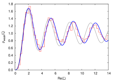
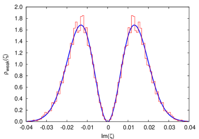
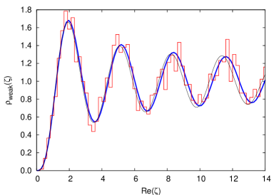
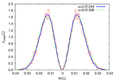
Figure 2: The scaling $\mu^{2}V$ for dynamical fermions: $V=6^{4}$, $ma=0.07$ and $\mu=1\cdot 10^{-3}$ $\Rightarrow$ $\alpha=0.013$, $\eta=33$ (upper plots) vs. $V=8^{4}$, $ma=0.07$ and $\mu=5.625\cdot 10^{-4}$ $\Rightarrow$ $\alpha=0.012$, $\eta=102$ (lower plots) .

We can now test the scaling hypothesis of $\mu^{2}$ eq. (2). For this purpose we have kept $\mu^{2}V$ fixed for the two volumes $V=6^{4}$ and $8^{4}$: $\mu=1\cdot 10^{-3}$ and $\mu=5.625\cdot 10^{-4}$, respectively. Since the level spacing $d$ also depends on the mass we have kept $ma$ fixed, leading automatically to different $\eta$-values for different volumes. The data (histograms) in Fig. 2 right confirm this scaling very well: the fitted $\alpha=0.013$ from $V=6^{4}$ (blue curve) describes the $V=8^{4}$ data as well (green). For $V=8^{4}$ we also display the $\alpha=0.012$ (blue) obtained from an independent fit, they agree within 5%. In the cuts in Fig. 2 left these small variations in $\alpha$ cannot be seen. If we were to compare to the quenched density a different fit value for $\alpha\sim 0.0185\ (6^{4})$ and $\alpha\sim 0.0175\ (8^{4})$ would be obtained instead, describing the right curves equally well. However, in the left plots the quenched MM curve (grey) deviates from the unquenched (blue) one. In the upper $V=6^{4}$ plot the discrepancy from $\eta=33$ to quenched can be clearly seen in the data as we capture up to the $4th$ maximum, whereas in $V=8^{4}$ keeping $ma$ fixed implies $\eta=102$, taking us back to almost quenched.

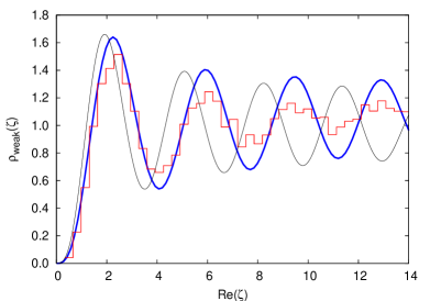
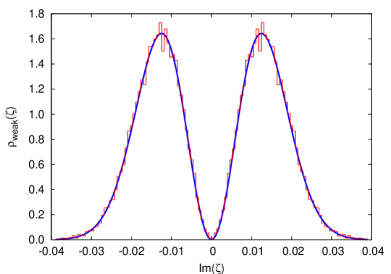
Figure 3: Data (histograms) vs. MM (blue curve=unquenched, grey=quenched) for $V=6^{4}$ $ma=0.035$ and $\mu=1\cdot 10^{-3}$ $\Rightarrow$ $\eta=14$ and $\alpha=0.012$.

In order to see the difference from quenched at smaller masses we compare to data corresponding to a rescaled mass $\eta=14$ (blue curve) in Fig. 3 below. Although we can only resolve well the first 2-3 maxima in the left picture, the mismatch with the quenched curve (grey) is evident.

To summarise we have shown that the MM correctly predicts complex $SU(2)$ Lattice data with $N_{f}=2$ dynamical staggered fermions at $\mu\neq 0$, describing the effect of small quark masses. We have also confirmed the scaling of $\mu^{2}$ with the volume at weak non-Hermiticity from unquenched Lattice data.

Acknowledgements: We thank Maria-Paola Lombardo, Harald Markum, Rainer Pullirsch and Tilo Wettig for helpful discussions and previous collaboration. This work was supported by a BRIEF Award No. 707 from Brunel University (G.A.) and by the Deutsche Forschungsgemeinschaft under grant No. JA483/17-3 (E.B.).

References

- [1] J.J.M. Verbaarschot, Phys. Rev. Lett. 72 (1994) 2531.
- [2] M.A. Halasz, J.C. Osborn and J.J.M. Verbaarschot, Phys. Rev. D56 (1997) 7059.
- [3] G. Akemann, Phys. Rev. Lett. 89 (2002) 072002; J. Phys. A: Math. Gen. 36 (2003) 3363.
- [4] K. Splittorff and J.J.M. Verbaarschot, Nucl. Phys. B683 (2004) 467.
- [5] G. Akemann, Y.V. Fyodorov and G. Vernizzi, Nucl. Phys. B694 (2004) 59.
- [6] J.C. Osborn, Phys. Rev. Lett. 93 (2004) 222001; private communication.
- [7] G. Akemann, J.C. Osborn, K. Splittorff and J.J.M. Verbaarschot Nucl. Phys. B712 (2005) 287.
- [8] G. Akemann, Nucl. Phys. B to appear [hep-th/0507156].
- [9] G. Akemann and T. Wettig, Phys. Rev. Lett. 92 (2004) 102002.
- [10] J.C. Osborn, Eigenvalue correlations in quenched QCD at finite density, these proceedings PoS(LAT2005)200.
- [11] G. Akemann, E. Bittner, M.-P. Lombardo, H. Markum and R. Pullirsch, Nucl. Phys. B140 Proc. Suppl. (2005) 568.
- [12] E. Bittner, M.-P. Lombardo, H. Markum and R. Pullirsch, Nucl. Phys. B106 Proc. Suppl. (2002) 468.
- [13] H. Markum, R. Pullirsch and T. Wettig, Phys. Rev. Lett. 83 (1999) 484.
- [14] E. Follana, Nucl. Phys. B140 Proc. Suppl. (2005) 141.
- [15] F. Karsch, Prog. Theor. Phys. Suppl. 153 (2004) 106.
- [16] S. Hands, J.B. Kogut, M.-P. Lombardo, and S.E. Morrison, Nucl. Phys. B 558 (1999) 327.
- [17] M.E. Berbenni-Bitsch, S. Meyer and T. Wettig, Phys. Rev. D58 (1998) 071502.
- [18] G. Akemann and E. Kanzieper, Phys. Rev. Lett. 85 (2000) 1174.
- [19] J. B. Kogut, M. A. Stephanov, D. Toublan, J. J. M. Verbaarschot and A. Zhitnitsky, Nucl. Phys. B582 (2000) 477.