Lattice QFT with FermiQCD

Abstract:

FermiQCD is a C++ library for fast development of parallel Lattice Quantum Field Theory computations. It has been developed following a top-down fully Object Oriented design approach with focus on simplicity of use. FermiQCD includes: a heatbath algorithm for Wilson and $O(a^{2})$ improved $SU(n)$ gauge actions; inversion algorithms for Wilson, Clover, Kogut-Susskind, Asqtad, and Domain Wall fermionic actions; example programs for various types of meson propagators; and converters for the most common gauge file formats.

PoS(LAT2005)104

1 INTRODUCTION

FermiQCD [1, 2, 3] is a library for fast development of parallel applications for Lattice Quantum Field Theories and Lattice Quantum Chromodynamics [4]. It was designed both to be easy to use, with a syntax very similar to common mathematical notation, and, at the same time, optimized for PC clusters.

FermiQCD takes a top-down approach: the top level functions were designed first, followed by optimized implementations of those functions. The most critical parts are optimized in assembler using SSE/SSE2 instructions. All FermiQCD algorithms are parallel but parallelization is hidden from the high level programmer. At the lowest level, parallelization is implemented in MPI and/or in PSIM. PSIM is a parallel emulator that allows running, testing and debugging of parallel code on a single processor PC without requiring MPI.

All components are implemented as separate, although related, classes. For example, in FermiQCD lattices and fields are objects while actions and inverters are static methods of the corresponding classes. FermiQCD components range from low level linear algebra, fitting and statistical functions (including the Bootstrap and a Bayesian fitter based on Levenberg-Marquardt minimisation) to high level parallel algorithms specifically designed for lattice quantum field theories such as the Wilson [5] and $O(a^{2})$-improved gauge actions, the Clover fermionic action, the Asqtad [6] action for KS fermions, and the Domain Wall action [7].

One can create a new action by creating a new class and plugging it into the rest the library. All other components, such as the inverters, will work with it. For example FermiQCD provides three inverters, MinRes, BiCGStab and UML. The first two are general and work with any action and any type of field, the third (UML) is highly optimized for KS and ASQTAD actions.

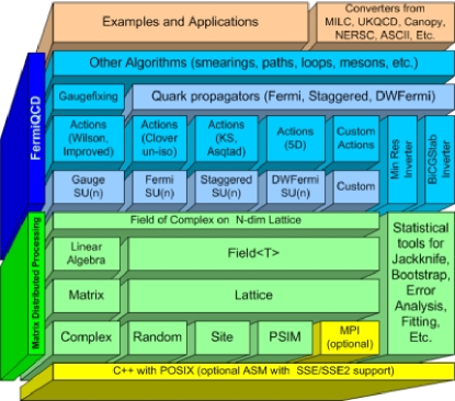
Figure 1: Components of FermiQCD.

Figure 1 shows a schematic representation of FermiQCD’s components. The lower components are referred to as Matrix Distributed Processing and they define the language used in FermiQCD. The upper components are the algorithms. The top components represent examples, applications and other tools. These tools include converters for the most gauge field formats: MILC, NERSC, UKQCD, CANOPY, and some binary formats.

2 SYNTAX OVERVIEW AND PROGRAM EXAMPLE

All FermiQCD algorithms are implemented on top of an Object Oriented Linear Algebra package with a Maple-like syntax. For example

$$A = \mathrm{trace}(\gamma^{2}(\gamma^{0}-\mathbf{1})/2)$$ (1)

$$B = e^{i\theta\lambda_{3}}$$ (2)

where $\gamma^{\mu}$ are the Dirac Gamma matrices in Euclidean space and $\lambda_{3}$ is one of the generators of $SU(3)$, are implemented in FermiQCD as

Complex A = trace(Gamma[i]*(Gamma[0]-1)/2);Matrix B = exp(I*theta*Lambda[3]);A $4D$ $16\times 8^{3}$ lattice is declared (with obvious generalization to arbitrary dimensions and sizes) as

int L[]={16,8,8,8};mdp_field lattice(4,L);An $SU(n)$ gauge field $U_{\mu}(x)$ is declared and initialized by

gauge_field U(lattice,n); set_cold(U);The following sets $\beta=6.0$ and performs 10 heatbath [8] steps with the Wilson gauge action

coefficients gauge; gauge["beta"]=6.0;WilsonGaugeAction::heatbath(U,gauge,10);

Any field can be saved: U.save("filename"); loaded: U.load("filename"); and translated: U.shift(mu);. A field can also be transformed locally. Here is how to implement a global gauge transformation $G$ of $U$

Matrix G=exp(2*I*Lambda[2]);mdp_site x(lattice);forallsites(x)   for(int mu=0; mu<U.ndim; mu++)      U(x,mu)=G*U(x,mu)*inv(G);U(x,mu) is an $n\times n$ matrix and x is an object that represents a lattice site. forallsites(x) is a parallel loop. Each processing node loops over the lattice sites stored by the node.

A Wilson fermionic field is declared as

fermi_field psi(lattice,n);and a gauge invariant shift can be implemented as

psi_up(x)=U(x,mu)*psi(x+mu);psi_dw(x)=hermitian(U(x-mu,mu))*psi(x-mu);Notice that x+mu reads as $x+\hat{\mu}$ and x-mu reads as $x-\hat{\mu}$ where $\mu=0,1,2,3$ is one of the possible lattice directions.

Multiplication by the fermionic matrix is invoked as follows

coefficients quark; quark["kappa"]=0.1245; quark["c_{SW}"]=0.0;if(quark["c_{SW}"]!=0) compute_em_field(U);default_fermi_action=FermiCloverActionFast::mul_Q;mul_Q(psi_out,psi_in,U,quark);The chromo-electromagnetic field is required by the clover term and computed only if required. It is stored inside a gauge field object. FermiQCD includes three different equivalent implementations of the above algorithm, declared in the following classes: FermiCloverActionSlow, FermiCloverActionFast, FermiCloverActionSSE2. The second is optimized in C++, the third is optimized in assembler.

The inverse multiplication $\psi_{\mathrm{out}}=Q^{-1}[U]\psi_{\mathrm{in}}$ is invoked with the following call

mul_invQ(psi_out,psi_in,U,quark,1e-20,1e-12);where 1e-20 is the target absolute precision for the numerical inversion and 1e-12 is the target relative precision.

An ordinary quark propagor is declared and generated by

fermi_propagator S(lattice,n);generate(S,U,quark,1e-20,1e-12);and it can be used, for example, to build a meson propagator $C_{\pi}(t)$ by summing the following expression over $x$ and over the spin components a, b

Cpi[x(TIME)]+=real(trace(S(x,a,b)*hermitian(S(x,a,b))));

Everything works similary for the other actions and other types of fields. Figure 2 shows a complete parallel program for generating nconfig gauge configurations in $SU(5)$ on a $16\times 8^{4}$ lattice, saving them and computing the average plaquette and the pion propagator on each configuration.

1#include "fermiqcd.h"

2int main(int argc, char **argv) {

3  mdp.open_wormholes(argc, argv);   // START

4  define_base_matrices("FERMIQCD"); // set Gamma convention

5  int n=5, nconfig=100;

6  int L[] = {16,8,8,8};

7  mdp_lattice lattice(4,L);         // declare lattice

8  gauge_field U(lattice, n);        // declare fields

9  fermi_propagator S(lattice,n);    // declare propagator

10  mdp_site x(lattice);              // declare a site var

11  coefficients gauge; gauge["beta"]=6.0; // set parameters

12  coefficients quark; quark["kappa"]=0.1234; quark["c_{SW}"]=0.0;

13  default_fermi_action=FermiCloverActionFast::mul_Q;

14  mdp_array<float,1> Cpi(L[TIME]);    // declare and zero Cpi

15  for(int t=0; t<L[TIME]; t++) Cpi(t)=0;

16  set_hot(U);

17  for(int k=0; k < nconfig; k++) {

18     WilsonGaugeAction::heatbath(U,gauge,10); // do heatbath

19     mdp << average_plaquette(U) << endl;     // print plaquette

20     U.save(string("gauge")+tostring(k));     // save config

21     if(quark["c_{SW}"]!=0) compute_em_field(U);

22     generate(S,U,quark,1e-20,1e-12);         // make propagator

23     forallsites(x)                           // contract pion

24       for(int a=0; a<4; a++)                 // source spin

25         for(int b=0; b<4; b++)               // sink spin

26           Cpi[x(TIME)]+=real(trace(S(x,a,b)*hermitian(S(x,a,b))));

27     mpi.add(Cpi.address(),Cpi.size());       // parallel add

28     for(int t=0; t<L[TIME]; t++)

29       mdp << t << " " << Cpi(t) << endl;     // print output

30  }

31  mdp.close_wormholes();            // STOP

32  return 0;

33 }

Figure 2: A complete parallel program in FermiQCD.

3 BENCHMARKS

Table 1 shows typical running times for the FermiQCD inverters applied to different actions. Times are in microsecond per lattice site per step. Notice that MinRes involves one mul_Q per step, BiCGStab involves two, and the UML inverter also involves two but only applied to sites of even parity. These times were computed on one 3.2GHz Pentiutm 4 (typical computations in parallel with a Myrinet network show a drop in efficiency of 20-30% when scaling up to 16-32 processors).

Action	Inverter	float	float (SSE)	double	double (SSE2)
Wilson	Min Res	8.83	1.79	6.84	2.07
Wilson	BiCGStab	17.8	3.16	13.8	4.42
Clover	Min Res	9.76	1.98	12.08	2.82
Clover	BiCGStab	19.63	4.71	24.95	6.08
KS	Min Res	1.42	0.78	1.71	1.01
KS	BiCGStab	2.95	1.63	3.56	2.11
KS	UML	1.89	1.14	2.08	1.34
Asqtad	Min Res	3.73	2.47	4.29	5.24
Asqtad	BiCGStab	7.65	5.02	8.79	6.61
Asqtad	UML	1.14	3.14	5.24	3.81

Table 1: Running times for FermiQCD inverters using different actions.

4 CONCLUSIONS

FermiQCD is now a stable and mature product and the project mailing list currently numbers more than 30 members. The Wilson and Asqtad inverters are as fast if not faster than any other software package available for PC clusters. FermiQCD is an Open Source project and users can contribute to its improvement by creating new classes and adding functionality. Some of our objectives include the addition of an optimized gauge action, optimized Domain Wall fermions, HMC for dynamical fermions, compatibility with the ILDG format [9], support for the SciDAC QMP API, and a GUI for visual development.

FermiQCD and additional documentation can be downloaded from: www.fermiqcd.net

References

- [1] M. Di Pierro, arXiv:hep-lat/0011083.
- [2] M. Di Pierro, Nucl. Phys. Proc. Suppl. 106, 1034 (2002) [arXiv:hep-lat/0110116].
- [3] M. Di Pierro et al. [FermiQCD Colaboration], Nucl. Phys. Proc. Suppl. 129, 832 (2004) [arXiv:hep-lat/0311027].
- [4] arXiv:hep-lat/0509013
- [5] K. G. Wilson, Phys. rev. D10 (1974) 2445
- [6] C. Bernard et al. [MILC Collaboration], Phys. Rev. D 58 (1998) 014503 [hep-lat/9712010].
- [7] D. B. Kaplan, Phys. Lett. B288 (1992) 342
- [8] M. Creutz, Phys. Rev. D21 2308 (1980)
- [9] B. Joo and W. Watson, Nucl. Phys. Proc. Suppl. 140, 209 (2005) [arXiv:hep-lat/0409165].