The Equation of State for QCD with 2+1 Flavors of Quarks

Abstract:

We report results for the interaction measure, pressure and energy density for nonzero temperature QCD with 2+1 flavors of improved staggered quarks. In our simulations we use a Symanzik improved gauge action and the Asqtad $O(a^{2})$ improved staggered quark action for lattices with temporal extent $N_{t}=4$ and 6. The heavy quark mass $m_{s}$ is fixed at approximately the physical strange quark mass and the two degenerate light quarks have masses $m_{ud}=0.1m_{s}$ or $0.2m_{s}$. The calculation of the thermodynamic observables employs the integral method where energy density and pressure are obtained by integration over the interaction measure.

PoS(LAT2005)156

1 Introduction

The equation of state (EOS) is important for phenomenological models of quark-gluon plasma formation and decay, which is currently under experimental study at RHIC and elsewhere. We have determined the EOS with the Asqtad quark action [1] for 2+1 flavors, combined with a one-loop Symanzik improved gauge action [2]. The Asqtad action is well suited for high temperature studies since it has excellent scaling properties and much better dispersion relations in the free case than the standard Wilson or staggered actions, which means decreased lattice artifacts above the transition.

Our nonzero temperature studies are at $N_{t}=4$ and 6. Even with Asqtad improvement, for $T\leq T_{c}$, an $N_{t}=4$ lattice has a badly split pion taste multiplet with some members heavier than the kaon, which makes for questionable strange quark physics. At $N_{t}=6$ the taste-splitting is about half as large. One of our goals was to determine to what extent the increase in $N_{t}$ from 4 to 6 influences the EOS.

2 Action

The fermion part of the action we use is effectively written as:

$$S_{f}=-\sum_{f}(n_{f}/4)\mbox{Tr}\ln[M(am_{f},U,u_{0})],$$ (1)

where $M(am_{f},U,u_{0})$ is the fermion matrix corresponding to the Asqtad 2+1 flavor staggered action. The gauge part is defined as:

$$S_{g}=\beta\sum_{x,\mu<\nu}(1-P_{\mu\nu})+\beta_{\rm rt}\sum_{x,\mu<\nu}(1-R_{\mu\nu})+\beta_{\rm ch}\sum_{x,\mu<\nu<\sigma}(1-C_{\mu\nu\sigma}).$$ (2)

The gauge couplings above are $\beta=10/g^{2}$, $\beta_{\rm rt}=-\beta(1+0.4805\alpha_{s})/(20u_{0}^{2})$, $\beta_{\rm ch}=-0.03325\beta\alpha_{s}/u_{0}^{2}$, with $\alpha_{s}=-4\ln(u_{0})/3.0684$ and $u_{0}=\left\langle P\right\rangle^{1/4}$.

For our simulations we use the dynamical R-algorithm [3] with step-size equal to the smaller of 0.02 and $2am_{ud}/3$. Our aim is to generate zero and nonzero temperature ensembles of lattices with action parameters chosen so that a constant physics trajectory ($m_{\pi}/m_{\rho}=const$) is approximated. Along the trajectory the heavy quark mass is fixed close to the strange quark mass. We work with two such trajectories: $m_{ud}=0.2m_{s}$ ($m_{\pi}/m_{\rho}\approx 0.4$) and $m_{ud}=0.1m_{s}$ ($m_{\pi}/m_{\rho}\approx 0.3$).

3 Parameterization of the Constant Physics Trajectories and Run Parameters

Our trajectories are intended to approximate constant zero temperature physics. The construction of each trajectory begins with ”anchor points” in $\beta$, where the hadron spectrum has been previously studied [4] and the lattice strange quark mass has been tuned to approximate the correct strange hadron spectrum. We adjusted the value of $am_{ud}$ at the anchor points to give a constant (unphysical) ratio $m_{\pi}/m_{\rho}$. Between these points the trajectory is then interpolated, using a one-loop renormalization group inspired formula. That is, we interpolate $\ln(am_{s})$ and $\ln(am_{ud})$ linearly in $\beta$. Since we have three anchor points for the $m_{ud}=0.2m_{s}$ trajectory, namely $\beta=6.467$, 6.76, and 7.092, our interpolation is piecewise linear. For the trajectory $m_{ud}=0.1m_{s}$ we use two anchor points at $\beta=6.458$ and 6.76. For both trajectories, for values of $\beta$ out of the interpolation intervals, the parameterization formulas are used as extrapolations appropriately. The run parameters of the two trajectories at different $N_{t}$ are summarized in Tables 1, 2 and 3.

$\beta$	$am_{ud}$	$am_{s}$	$u_{0}$	$V_{T\neq 0}$	$V_{T=0}$
⋆6.300	0.0225	0.1089	0.8455	$12^{3}\times 6$	$12^{4}$
⋆6.350	0.0206	0.1001	0.8486	$12^{3}\times 6$	$12^{4}$
6.400	0.01886	0.0919	0.8512	$12^{3}\times 6$
6.433	0.01780	0.0870	0.8530	$12^{3}\times 6$
⋆6.467	0.01676	0.0821	0.8549	$16^{3}\times 6$	$16^{3}\times 48$
6.500	0.01580	0.0776	0.8568	$12^{3}\times 6$
⋆6.525	0.01510	0.0744	0.8580	$12^{3}\times 6$	$12^{4}$
6.550	0.01450	0.0713	0.8592	$12^{3}\times 6$
⋆6.575	0.01390	0.0684	0.8603	$12^{3}\times 6$	$16^{4}$
6.600	0.01330	0.0655	0.8614	$12^{3}\times 6$
⋆6.650	0.01210	0.0602	0.8634	$12^{3}\times 6$	$20^{4}$
6.700	0.01110	0.0553	0.8655	$12^{3}\times 6$
⋆6.760	0.01000	0.0500	0.8677	$20^{3}\times 6$	$20^{3}\times 64$
7.092	0.00673	0.0310	0.8781	$12^{3}\times 6$
7.090	0.00620	0.0310	0.8782		$28^{3}\times 96$

Table 1: Run parameters of the trajectory with $m_{ud}=0.2m_{s}$ at $N_{t}=6$. The asterisk indicates parameter sets for which both zero and nonzero temperature runs were performed.

$\beta$	$am_{ud}$	$am_{s}$	$u_{0}$	$V_{T\neq 0}$	$V_{T=0}$
⋆6.300	0.01090	0.1092	0.8459	$12^{3}\times 6$	$12^{4}$
⋆6.350	0.00996	0.0996	0.8491	$12^{3}\times 6$	$12^{4}$
6.400	0.00909	0.0909	0.8520	$12^{3}\times 6$
⋆6.458	0.00820	0.0820	0.8549	$16^{3}\times 6$	$12^{4}$
6.500	0.00765	0.0765	0.8570	$12^{3}\times 6$
⋆6.550	0.00705	0.0705	0.8593	$12^{3}\times 6$	$20^{4}$
6.600	0.00650	0.0650	0.8616	$12^{3}\times 6$
⋆6.650	0.00599	0.0599	0.8636	$12^{3}\times 6$	$24^{4}$
6.700	0.00552	0.0552	0.8657	$12^{3}\times 6$
⋆6.760	0.00500	0.0500	0.8678	$20^{3}\times 6$	$24^{3}\times 64$
⋆7.080	0.00310	0.0310	0.8779	$18^{3}\times 6$	$40^{3}\times 96$

Table 2: Run parameters of the trajectory with $m_{ud}=0.1m_{s}$ at $N_{t}=6$. The asterisk indicates parameter sets for which both zero and nonzero temperature runs were performed.

$\beta$	$am_{ud}$	$am_{s}$	$u_{0}$	$V_{T\neq 0}$	$V_{T=0}$
⋆6.000	0.01980	0.1976	0.8250	$12^{3}\times 4$	$12^{4}$
⋆6.050	0.01780	0.1783	0.8282	$12^{3}\times 4$	$12^{4}$
6.075	0.01690	0.1695	0.8301	$12^{3}\times 4$
⋆6.100	0.01610	0.1611	0.8320	$12^{3}\times 4$	$12^{4}$
6.125	0.01530	0.1533	0.8338	$12^{3}\times 4$
⋆6.150	0.01460	0.1458	0.8356	$12^{3}\times 4$	$12^{4}$
6.175	0.01390	0.1388	0.8374	$12^{3}\times 4$
⋆6.200	0.01320	0.1322	0.8391	$12^{3}\times 4$	$12^{4}$
6.225	0.01260	0.1260	0.8407	$12^{3}\times 4$
⋆6.250	0.01200	0.1201	0.8424	$12^{3}\times 4$	$12^{4}$
6.275	0.01140	0.1145	0.8442	$12^{3}\times 4$
⋆6.300	0.01090	0.1092	0.8459	$12^{3}\times 4$	$12^{4}$
⋆6.350	0.00996	0.0996	0.8491	$12^{3}\times 4$	$12^{4}$
6.400	0.00909	0.0909	0.8520	$12^{3}\times 4$
⋆6.458	0.00820	0.0820	0.8549	$12^{3}\times 4$	$12^{4}$
6.500	0.00765	0.0765	0.8570	$12^{3}\times 4$
⋆6.550	0.00705	0.0705	0.8593	$12^{3}\times 4$	$20^{4}$
6.600	0.00650	0.0650	0.8616	$12^{3}\times 4$
⋆6.650	0.00599	0.0599	0.8636	$12^{3}\times 4$	$24^{4}$
6.700	0.00552	0.0552	0.8657	$12^{3}\times 4$
⋆6.760	0.00500	0.0500	0.8678	$12^{3}\times 4$	$24^{3}\times 64$

Table 3: Run parameters of the trajectory with $m_{ud}=0.1m_{s}$ at $N_{t}=4$. The asterisk indicates parameter sets for which both zero and nonzero temperature runs were performed.

4 Integral Method for the EOS derivation

To derive the analytic form of the EOS we employ the integral method [5]. We start from the thermodynamic identities:

$$\varepsilon V=-\left.\frac{\partial\ln Z}{\partial(1/T)}\right|_{V},\hskip 19.91684pt\frac{p}{T}=\left.\frac{\partial\ln Z}{\partial V}\right|_{T}\approx\frac{\ln Z}{V},\hskip 19.91684ptI=\varepsilon-3p=-\frac{T}{V}\frac{\partial\ln Z}{\partial\ln a},$$ (3)

where the derivative with respect to $\ln a$ is taken at constant $m_{\pi}/m_{\rho}$ and the partition function is $Z$. Using the above identities and the explicit form of $Z$ we obtain:

$$Ia^{4} = -6\frac{d\beta}{d\ln a}\Delta\left\langle P\right\rangle-12\frac{d\beta_{\rm rt}}{d\ln a}\Delta\left\langle R\right\rangle-16\frac{d\beta_{\rm ch}}{d\ln a}\Delta\left\langle C\right\rangle$$

$$- \sum_{f}\frac{n_{f}}{4}\left[\frac{d(m_{f}a)}{d\ln a}\Delta\left\langle\bar{\psi}\psi\right\rangle_{f}+\frac{du_{0}}{d\ln a}\Delta\left\langle\bar{\psi}\,\frac{dM}{du_{0}}\,\psi\right\rangle_{f}\right],$$

$$pa^{4} = \int_{\ln a_{0}}^{\ln a}\left\{6\frac{d\beta}{d\ln a}\Delta\left\langle P\right\rangle+12\frac{d\beta_{\rm rt}}{d\ln a}\Delta\left\langle R\right\rangle+16\frac{d\beta_{\rm ch}}{d\ln a}\Delta\left\langle C\right\rangle\right.$$

$$+ \left.\sum_{f}\frac{n_{f}}{4}\left[\frac{d(m_{f}a)}{d\ln a}\Delta\left\langle\bar{\psi}\psi\right\rangle_{f}+\frac{du_{0}}{d\ln a}\Delta\left\langle\bar{\psi}\,\frac{dM}{du_{0}}\,\psi\right\rangle_{f}\right]\right\}\,d\ln a^{\prime},$$

$$\varepsilon a^{4} = (I+3p)a^{4}.$$ (6)

In the above expressions the symbol $\Delta$ in front of the lattice observables stands for the difference between the values of those observables at nonzero and zero temperatures. In the pressure expression, the lower integration endpoint $\ln a_{0}$ is set where the zero temperature subtracted value of $Ia^{4}$ is zero within errors at coarse lattice spacings. To calculate the EOS, in addition to the lattice gluonic and fermionic observables in the above analytic forms, we need to calculate the derivatives $d\beta_{\rm pl}/d\ln a$, $d\beta_{\rm rt}/d\ln a$, $d\beta_{\rm ch}/d\ln a$, $d(m_{f}a)/d\ln a$ and $du_{0}/d\ln a$. For this purpose we take derivatives of the $\ln(am_{ud})$ and $\ln(am_{s})$ trajectory parameterizations, polynomial fits to $u_{0}(\beta)$ for both trajectories, and the updated version of the $\ln(r_{1}/a)$ fitting formula in [4] shown below:

$$\ln(r_{1}/a) = C_{00}+C_{10}(\beta-7)+C_{21}(2am_{ud}+am_{s})+C_{20}(\beta-7)^{2},$$ (7)

where $r_{1}=0.317(7)(3)$ fm, $C_{00}=1.261(3)$, $C_{10}=0.939(8)$, $C_{21}=-0.86(3)$ and $C_{20}=-0.25(2)$. The above fit (4.5) giving the relative lattice scale is based on measurements of the static quark potential at zero temperature for a large set of $\beta$ and quark masses. The absolute scale is fixed from a determination of the bottomonium spectrum [6]. The fit has $\chi^{2}/DOF\approx 1.1$.

5 EOS results

Figure 1 summarizes our results for the EOS. The errors on all data points are calculated using the jackknife method, and we ignore insignificant errors on the derivatives of the bare parameters with respect to the lattice scale discussed at the end of the previous section. For the points where there is no zero temperature run, local interpolations are made to calculate the zero temperature corrections to the interaction measure. The integration of the interaction measure to obtain the pressure is done using the trapezoid method.

The comparison between the $N_{t}=4$ and 6 cases for the $m_{ud}=0.1m_{s}$ trajectory shows that there is not a significant difference between them, except in the interaction measure near the transition region. The EOS results from the two different physics trajectories are very similar and for the temperature interval we studied, the deviation from the 3 flavor Stefan–Boltzmann values are large.

In the temperature region where we have data, we consider our pressure results to be in general agreement to a previous p4-action $N_{t}=4$ calculation [7].

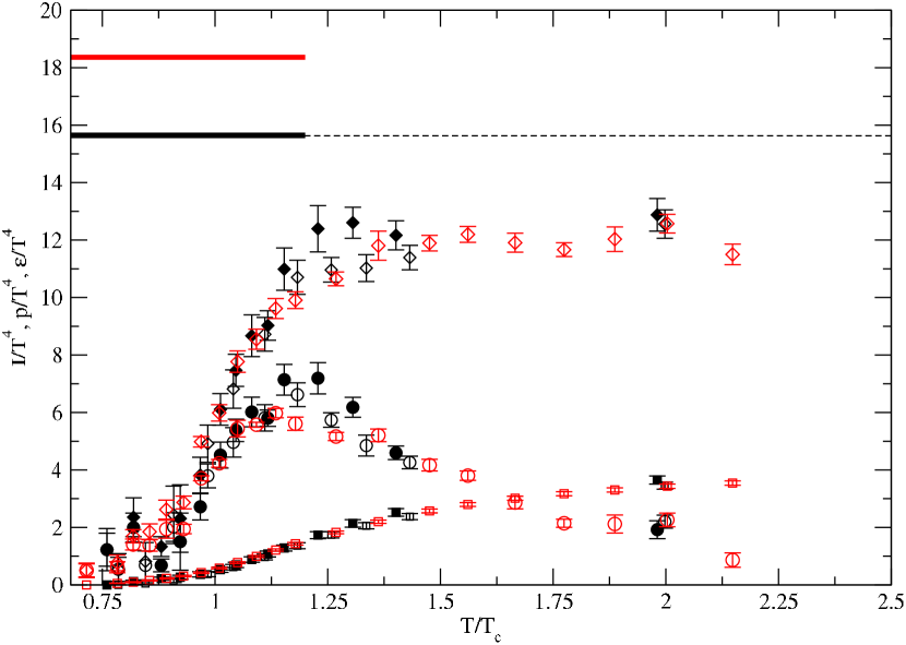
Figure 1: The EOS with 2+1 dynamical quark flavors for both constant physics trajectories. The energy density, pressure and the interaction measure symbols are diamonds, squares and circles, respectively. The data at $N_{t}=6$ is in black and at $N_{t}=4$ in red. All data with filled symbols belong to the $m_{ud}=0.2m_{s}$ trajectory and the empty symbols belong to the $m_{ud}=0.1m_{s}$ trajectory. The Stefan–Boltzmann lattice limits for 3 flavors of quarks at $N_{t}=4$ and 6 are represented by solid lines – red and black, respectively. The black dashed line is the continuum Stefan–Boltzmann limit for 3 flavors of quarks.

6 Conclusions

We have calculated the EOS for 2+1 dynamical flavors of improved staggered quarks ($m_{ud}/m_{s}=0.1$ and 0.2) along trajectories of constant physics, at $N_{t}=4$ and 6, where the latter is the first result of its kind. Our results show that the $N_{t}=4$ and $N_{t}=6$ results are quite similar except in the crossover region where the interaction measure is a bit higher on the finer $N_{t}=6$ lattice. We also do not see significant differences between the EOS results from the two physics trajectories. We find large deviations from the 3 flavor Stefan–Boltzmann limit. Our results are comparable with previous calculations [7].

Acknowledgments

This work was supported by the US DOE and NSF. Computations were performed at CHPC (Utah), FNAL, FSU, IU, NCSA and UCSB.

References

- [1] K. Orginos and D. Toussaint, Testing improved actions for dynamical Kogut-Susskind quarks, Phys. Rev. D59 (1999) 014501; Tests of improved Kogut-Susskind fermion actions, Nucl. Phys. (Proc. Suppl.) 73 (1999) 909; G. P. Lepage, Perturbative improvement for lattice QCD: An update, Nucl. Phys. (Proc. Suppl.) 60A (1998) 267-278; Flavor symmetry restoration and Symanzik improvement for staggered quarks, Phys. Rev. D 59 (1999) 074502.
- [2] K. Symanzik, Recent developments in gauge theories, eds. G. ‘t Hooft et al., Plenum, New York 1980, 313.
- [3] S. Gottlieb et al., Hybrid molecular dynamics algorithms for the numerical simulation of quantum chromodynamics, Phys. Rev. D35 (1987) 2531–2542.
- [4] C. Aubin et al., Light hadrons with improved staggered quarks: approaching the continuum limit, Phys. Rev. D70 (2004) 094505.
- [5] J. Engels et al., Non-perturbative thermodynamics of SU(N) gauge theories, Phys. Lett. 252 (1990) 625–630.
- [6] M. Wingate et al., The and decay constants in 3 flavor lattice QCD, Phys. Rev. Lett. 92 (2004) 162001. A. Gray et al., The spectrum and from full lattice QCD, [hep-lat/0507013].
- [7] F. Karsch et al., The pressure in 2, 2+1 and 3 flavour QCD, Phys. Lett. B478 (2000) 447–455.