Another weak first order deconfinement transition: three-dimensional $SU(5)$ gauge theory
Kieran Holland

Department of Physics, University of California San Diego,

9500 Gilman Drive, La Jolla CA 92093, USA

Abstract

We examine the finite-temperature deconfinement phase transition of $(2+1)$-dimensional $SU(5)$ Yang-Mills theory via non-perturbative lattice simulations. Unsurprisingly, we find that the transition is of first order, however it appears to be weak. This fits naturally into the general picture of “large” gauge groups having a first order deconfinement transition, even when the center symmetry associated with the transition might suggest otherwise.

1 Motivation

Yang-Mills theory, of self-interacting gluons, is not a full description of the strong interaction occurring in Nature, but even on its own it is remarkably rich. At low temperatures, it is a confining theory, describing a world of color-neutral particles. At high temperatures, Yang-Mills theory describes weakly-interacting color-charged deconfined particles in a plasma. This exactly mimics the behavior of QCD. However, unlike QCD, pure gauge theory has an exact global symmetry associated with the change from a confining to a deconfining theory, giving a strict finite-temperature phase transition. For a more general gauge theory where the number of gluons is increased e.g. $SU(N)$, there are hints of a simpler description in terms of string dynamics in the limit $N\rightarrow\infty$ [1], a limit which appears surprisingly close to the real world with $N=3$ [2]. There is evidence of an effective string theory which describes the excitations of the color flux tube, the QCD string, in the confined phase of the gauge theory [3]. Yang-Mills theory is also a testing ground for ideas about what are the relevant degrees of freedom that lead to confinement, possible candidates being center vortices, monopoles, instantons or other topological features [4]. From a practical viewpoint, lattice simulations of pure gauge theory are much less computationally intensive than those of full QCD, allowing some questions to be answered in greater detail.

The global symmetry relevant for the deconfinement transition in pure gauge theory is the center symmetry [5]. Finite-temperature $T$ in the gauge theory means the Euclidean time direction is of finite extent $1/T$ and physical quantities are periodic in this direction. For gauge group $G$, the gauge fields themselves are only periodic in the time direction up to a gauge transformation. The gauge transformations can be twisted globally by $z\in H$, the center of the group $G$. The center is the largest subgroup whose elements commute with all elements of the full group. This is an exact global symmetry of Yang-Mills theory at finite temperature. At low temperatures, the theory is confining and the center symmetry is intact. At the critical temperature $T_{c}$ where the theory becomes deconfining, the center symmetry is spontaneously broken. Hence deconfinement in pure gauge theory is a strict phase transition. Quarks break the center symmetry explicitly, so the switch from confinement to deconfinement in QCD is a crossover.

Over the years, the finite-temperature deconfinement phase transition in Yang-Mills theory has been studied in great detail and non-perturbative lattice simulations have played a decisive role. One can test ideas about the deconfinement transition by varying the gauge group and the space-time dimensionality. Let us summarize what is currently known. If the deconfinement transition is of second order, with a diverging correlation length $\xi$, Svetitsky and Yaffe conjectured that the universal properties of the transition are identical to those of the ordering transition of a spin model in one lower dimension. In particular, the symmetry of the spin system is the center of the gauge group [6]. For $SU(N)$, the center is $Z(N)$, the complex $N$-th roots of 1. In $(3+1)$ dimensions, $SU(2)$ gauge theory does have a second order deconfinement transition [7] and its universal properties, e.g. how the correlation length diverges near the critical temperature,

$$\xi\propto(T-T_{c})^{-\nu},$$ (1)

are identical to those of the 3-dimensional $Z(2)$-symmetric spin system i.e. the Ising model [8]. Most relevant to Nature, $(3+1)$-dimensional $SU(3)$ gauge theory has a weak first order deconfinement transition with a large but finite correlation length [9], and the Svetitsky-Yaffe conjecture does not apply. Continuing this sequence in $(3+1)$ dimensions, $SU(N)$ gauge theories continue to have first order deconfinement transitions for $N\geq 4$, with the transition becoming stronger as $N$ increases [10]. In $(2+1)$ dimensions, the story is somewhat different, with $SU(2)$ and $SU(3)$ gauge theories both having second order transitions, belonging to the universality classes of the 2-dimensional $Z(2)$- and $Z(3)$-symmetric spin models respectively [11]. For $SU(4)$ the transition appears very weak but it is not possible to rule out that it is first order, especially as the $Z(4)$ universality class has a set of continuously varying critical exponents [12].

It is clear that $(3+1)$-dimensional $SU(N)$ gauge theory has a deconfinement transition that switches from second to first order as $N$ increases. However, as the center $Z(N)$ also varies, it’s not possible to separate the size of the group from the change in the center symmetry. An alternate sequence one can consider is that of the symplectic groups $Sp(N)$, whose center is $Z(2)$ for all $N$. The group $Sp(N)$ has $N(2N+1)$ generators and there is a common member $Sp(1)=SU(2)$. Hence one can study the effect of the size of the group on the deconfinement transition without changing the symmetry class. What was found is somewhat surprising [13]. In $(3+1)$ dimensions, the $Sp(N)$ deconfinement transition changes from second to first order going from $N=1$ to $N=2$. In $(2+1)$ dimensions, $Sp(N)$ gauge theory has second order deconfinement transitions for $N=1$ and 2, but it becomes first order for $N=3$. All second order transitions belong to the expected $Z(2)$ universality class. This is the same qualitative behavior as for $SU(N)$, but in this case the center symmetry is unchanged and one might a priori expect the nature of the deconfinement transition to be the same for all gauge groups.

A crude argument one can make in favor of first order deconfinement transitions for large groups is the mismatch of degrees of freedom at the critical temperature. As the size of the group increases, so does the number of deconfined gluons in the plasma phase, while the number of color-neutral states in the confined phase is unchanged. The results for $Sp(N)$ indicate that the size of the group seems to dictate the order of the transition, as the $Z(2)$ universality class is available for all $N$, but the gauge theory chooses not to avail of it as $N$ increases. The situation is actually similar for $SU(N)$ in $(3+1)$ dimensions. It turns out that the ordering transitions of 3-dimensional $Z(N)$-symmetric spin models for $N\geq 5$ all belong to the universality class of the 3-dimensional $U(1)$-symmetric $XY$ model: the $Z(N)$ symmetry is enhanced to $U(1)$ at the critical point [14]. However, the $SU(N)$ gauge theories have first order deconfinement transitions for $N\geq 3$ and choose not to utilise the available universality class. A further surprise is given by the exceptional group $G(2)$, which has 14 generators and whose center is trivially 1. With a trivial center, there is no distinction between the confined and deconfined phases and one would expect the deconfinement transition to be a crossover without any singularity [15]. In fact, it appears that $(3+1)$-dimensional $G(2)$ gauge theory actually has an unexpected first order finite-temperature deconfinement transition [16]. Again, the size of the group, measured for example by the number of generators, seems to drive the transition first order, independent of the symmetry associated with the transition.

The purpose of this paper is to add one more datum to this collection of results. We examine $SU(5)$ gauge theory in $(2+1)$ dimensions, the smallest group which has not yet been studied in this space-time. Comparing to the known results for $SU(N)$ and $Sp(N)$ gauge theory, one would expect the $SU(5)$ deconfinement transition to be of first order. The $SU(4)$ transition is very weak and possibly belongs to the $Z(4)$ universality class, but could also be first order. The $Sp(3)$ deconfinement transition is weak but clearly of first order. A first order transition for $SU(5)$ would be consistent with the general notion that the size of the group dictates the order of the transition, and we test the idea with this study. There are additional reasons to expect a first order deconfinement transition for this theory. The relevant spin model for $SU(5)$ is the 2-dimensional $Z(5)$-symmetric spin model, for which no universality class is known. In fact, the ordering transition of the $Z(N)$ Potts model in 2 dimensions is of first order for $N\geq 5$ [17]. Interestingly, the correlation length of the Potts model at the critical point behaves as [18]

$$\xi=\frac{1}{8\sqrt{2}}x(1+{\cal O}(\frac{1}{x^{2}})),\hskip 21.33955ptx=\exp(\frac{\pi^{2}}{2\ln\frac{1}{2}(\sqrt{N}+\sqrt{N-4})}).$$ (2)

which diverges as $N\rightarrow 4^{+}$ and is already on the order of a few thousand lattice spacings for $N=5$, indicating a very weak first order transition. This might be an indication that the deconfinement transition of the gauge theory is first order but weak. In any event, we wish to rule out any surprises by establishing the nature of the gauge theory transition using lattice simulations.

In the course of writing this paper, we learnt of related work by Liddle and Teper investigating the deconfinement transition of $SU(N)$ gauge theories in $(2+1)$ dimensions for $N=4,5$ and 6 [19]. We believe they come to the same conclusion that $SU(5)$ gauge theory has a first order transition.

2 Lattice details

We perform standard lattice simulations of $(2+1)$-dimensional $SU(5)$ gauge theory. We use a finite periodic lattice volume of size $L^{2}\times L_{t}$ and lattice spacing $a$. The fundamental variables are gauge links $U_{x,\mu}$ which are elements of the group $SU(5)$. We use the standard Wilson plaquette gauge action

$$S[U]=\frac{10}{g^{2}}\sum_{\Box}(1-\frac{1}{5}{\rm ReTr}U_{\Box})=\frac{10}{g^{2}}\sum_{x,\mu<\nu}(1-\frac{1}{5}{\rm ReTr}(U_{x,\mu}U_{x+\hat{\mu},\nu}U^{\dagger}_{x+\hat{\nu},\mu}U^{\dagger}_{x,\nu})),$$ (3)

where $g$ is the bare gauge coupling. The partition function is

$$Z=\int{\cal D}U\exp(-S[U]),\hskip 21.33955pt\int{\cal D}U=\prod_{x,\mu}\int_{SU(5)}dU_{x,\mu}.$$ (4)

Finite temperature $T$ in the gauge theory is related to the periodic Euclidean time extent as $L_{t}a=1/T$. The relevant observable to examine the finite-temperature deconfinement transition is the complex-valued Polyakov loop [20],

$$\Phi_{\vec{x}}={\rm Tr}({\cal P}\prod_{t=1}^{L_{t}}U_{(\vec{x},t),3}),$$ (5)

given by a path-ordered product of the time-like gauge links. The gauge links in the time direction are periodic up to a gauge transformation. The gauge transformation itself need not be periodic but can be twisted by $z\in Z(5)$. This center rotation leaves the action $S$ unchanged, hence this is an exact symmetry of the theory. However the Polyakov loop picks up the twist $\Phi_{\vec{x}}\rightarrow z\Phi_{\vec{x}}$ because it wraps completely around the finite time direction, so it is sensitive to the center. The Polyakov loop expectation value,

$$\langle\Phi\rangle=\frac{1}{Z}\int{\cal D}U\frac{1}{L^{2}}\sum_{\vec{x}}\Phi_{\vec{x}}\exp(-S[U]),$$ (6)

measures the free energy $F$ at finite temperature $T$ of a static test quark sitting in the box, $\langle\Phi\rangle=\exp(-F/T)$. In the confined phase without isolated color-charged particles, the quark free energy diverges, $\langle\Phi\rangle=0$ and the center symmetry is intact, since $\langle\Phi\rangle=0=\langle z\Phi\rangle$. Above the critical temperature $T_{c}$ where the theory becomes deconfining, color-charged particles in the plasma have a finite free energy, $\langle\Phi\rangle\neq 0$ and the center symmetry is spontaneously broken. Hence the deconfinement transition can be identified via the behavior of the Polyakov loop.

3 Simulation results

We use standard methods in our lattice simulations. With the Wilson gauge action, we generate ensembles of gauge configurations using heat-bath [21] and over-relaxation [22] algorithms to update the various $SU(2)$ subgroups of the $SU(5)$ gauge links [23]. One can update all possible $SU(2)$ subgroups, but this is likely to be an overkill and in practice we update five randomly chosen subgroups. One sweep of the lattice volume corresponds to one heat-bath and four over-relaxation updates of every gauge link.

The lattice spacing $a$ is implicitly determined by the bare gauge coupling $\beta=10/g^{2}$ and the continuum limit is approached by taking $\beta\rightarrow\infty$. In practice one simulates at a number of $\beta$ values and tries to extrapolate results to the continuum. One has to beware of any possible unphysical transitions in the theory at finite $\beta$. If such a bulk transition exists, this sets a lower limit on $\beta$ i.e. an upper limit on the coarsest lattice spacing one can use and still make a connection to continuum physics. In Fig. 1 we plot the expectation value of the plaquette as a function of the bare gauge coupling on $6^{3}$ volumes. We use both ordered (“cold”) and random (“hot”) initial gauge configurations when generating the ensembles, which we see give completely consistent results. We see no sign of a bulk phase transition, which would be indicated by a jump in the plaquette average. One can analytically calculate the plaquette expectation value at weak and strong coupling, which to leading order give

$$\frac{1}{5}\langle{\rm ReTr}U_{\Box}\rangle = 1-8/\beta\hskip 14.22636pt({\rm large}~{}\beta)$$ (7)

$$= \beta/50\hskip 14.22636pt({\rm small}~{}\beta).$$

We see that both expansions match excellently the simulation results. For calibration, we give some of the plaquette expectation values in Table 1.

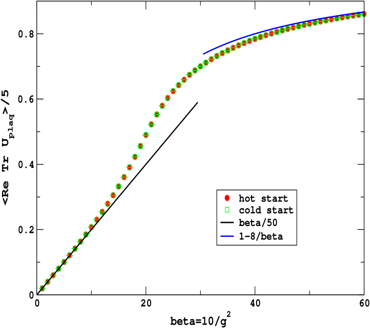
Figure 1: The plaquette expectation value $\langle{\rm ReTr}U_{\Box}\rangle/5$ versus the gauge coupling $\beta=10/g^{2}$. The curves are the lowest order expansions for small and large $\beta$. The errors for the data are much smaller than the symbol size.

In our simulations to determine the nature of the phase transition, we consider $L_{t}=3,4$ and 5 and take the spatial extent as large as $L=48$. For each $L_{t}$, there is a critical gauge coupling $\beta_{c}$ which determines the lattice spacing corresponding to the critical temperature $T_{c}=1/L_{t}a(\beta_{c})$. Increasing $L_{t}$, the lattice spacing at the critical temperature is reduced and the continuum limit is approached. In our production runs, for each $\beta$ value and lattice volume we perform at least 100,000 sweeps to generate the ensemble of gauge configurations.

The Polyakov loop expectation value $\langle\Phi\rangle$ is the order parameter which tells us if the system is in the confined or deconfined bulk phase. In Fig. 2, we plot the Monte Carlo history of the Polyakov loop average configuration by configuration for a particular lattice size and temperature (the history is the sequence of gauge configurations generated by the updating algorithms). The gauge coupling is chosen such that the temperature is close to criticality. Because of the $Z(5)$ center symmetry, there are five deconfined bulk phases distinguished by $\Phi$. We see that the system spends long periods in one bulk phase before rapidly tunneling to another one. In addition to the periods where $\Phi\neq 0$, the system spends a considerable fraction of the time fluctuating around $\Phi\approx 0$.

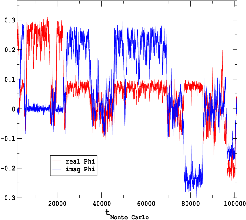
Figure 2: The Monte Carlo history of the complex-valued Polyakov loop $\Phi$. The lattice size is $40^{2}\times 3$ and the gauge coupling $\beta=32.0513$, which is close to the critical coupling for this volume. The system spends long periods in different bulk phases separated by rapid tunnelings.

Because we work at finite volume, the Polyakov loop average over all gauge configurations will vanish, independently of the temperature, as the system can tunnel between all possible bulk phases. Only in the infinite-volume limit is the tunneling suppressed and $\langle\Phi\rangle\neq 0$. This makes it difficult to locate the critical temperature where the transition occurs. To eliminate this problem, we use the modulus $\langle|\Phi|\rangle$ to identify the bulk phases. This quantity is always non-zero but as the volume increases $\langle|\Phi|\rangle$ ultimately vanishes in the confined phase and remains non-zero in the deconfined phase. In Fig. 3 we plot the probability distribution of $|\Phi|$ for the ensemble shown in Fig. 2. We see a clear double-peaked distribution, where we identify the inner and outer peaks with the confined and deconfined bulk phases respectively. The deconfined phase is slightly preferred, so the temperature is probably slightly above criticality. The most important information is that it looks like there is clearly coexistence of the confined and deconfined phases at the critical temperature. This is an obvious signal of a first order deconfinement transition.

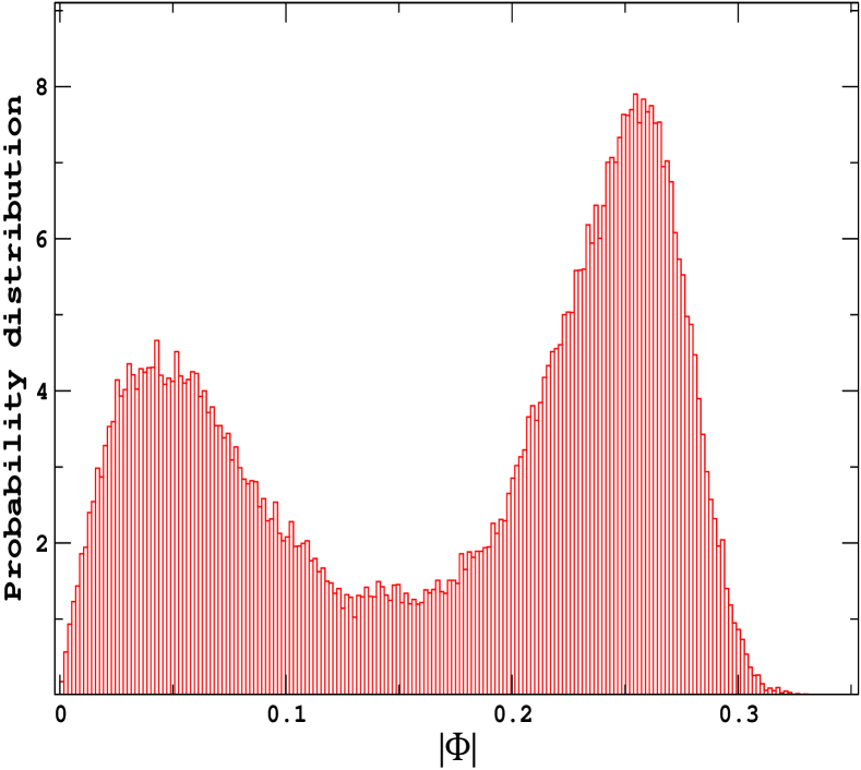
Figure 3: The probability distribution of $|\Phi|$ in a volume of size $40^{2}\times 3$ and gauge coupling $\beta=32.0513$, close to criticality. The double-peaked distribution indicates a first order phase transition.

To make the observation more quantitative, we measure the susceptibility of the Polyakov loop

$$\chi=L^{2}[\langle|\Phi|^{2}\rangle-\langle|\Phi|\rangle^{2}].$$ (8)

The susceptibility is maximized at a temperature which we use to define the finite-volume critical coupling $\beta_{c,V}$. This will differ from other definitions of the critical coupling, but all methods should agree in the infinite-volume limit. In addition, if the deconfinement transition is of first order, the rescaled susceptibility maximum $\chi_{\rm max}/L^{2}$ should be non-zero as $L\rightarrow\infty$.

For each lattice volume, we perform simulations at a number of gauge couplings $\beta$. To determine where the susceptibility attains a maximum, we use the standard reweighting method [24]. A number of ensembles over a range of $\beta$ values are combined allowing us to interpolate the value of $\chi$ for intermediary $\beta$ values. This method works excellently provided there is sufficient overlap among the different ensembles. In Fig. 4 we plot a typical result using this method. This allows for an accurate determination of the critical coupling $\beta_{c,V}$ at the susceptibility peak.

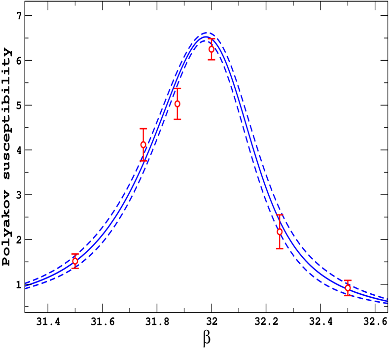
Figure 4: The Polyakov loop susceptibility $\chi$ versus the gauge coupling. The data are obtained from separate simulations and the curves are obtained using standard reweighting to combine the various ensembles. The lattice volume is $28^{2}\times 3$.

In Fig. 5 we plot the finite-volume critical couplings $\beta_{c,V}$ determined via reweighting for $L_{t}=3$. We extrapolate to the infinite-volume limit using the ansatz

$$\beta_{c,V}=\beta_{c,\infty}+a_{0}\frac{L_{t}^{2}}{L^{2}},$$ (9)

which we see is in very good agreement with the data. For the extrapolation of the susceptibility peak, we use the fitting form

$$\frac{\chi_{\rm max}}{L^{2}}=(\frac{\chi_{\rm max}}{L^{2}})_{\infty}+b_{0}\frac{L_{t}^{2}}{L^{2}}.$$ (10)

The data and extrapolation of $\chi_{max}/L^{2}$ for $L_{t}=3$ are plotted in Fig. 6. The fit is reasonable although the data is not very precisely measured. More importantly, the peak susceptibility in the infinite-volume limit $(\chi_{\rm max}/L^{2})_{\infty}$ is clearly non-zero. This is further evidence that the deconfinement phase transition is of first order.

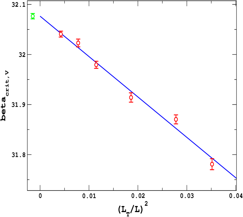
Figure 5: The infinite-volume extrapolation of the critical coupling $\beta_{c,V}$ for $L_{t}=3$, using a $1/L^{2}$ ansatz. The extrapolated value $\beta_{c,\infty}$ is shown slightly offset to the left.

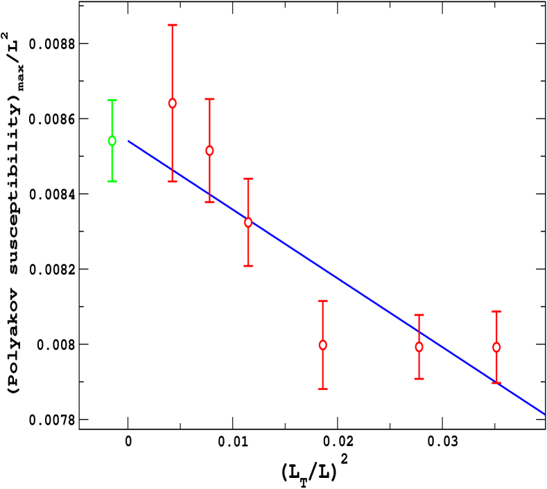
Figure 6: The infinite-volume extrapolation of the susceptibility maximum $\chi_{\rm max}/L^{2}$, using a $1/L^{2}$ ansatz. The extrapolated value $(\chi_{\rm max}/L^{2})_{\infty}$ is slightly offset to the left.

We find very similar results for $L_{t}=4$ and 5, namely clear double-peaked distributions of $|\Phi|$ and a non-zero extrapolated value for the peak susceptibility $(\chi_{\rm max}/L^{2})_{\infty}$. This is good evidence that the first order deconfinement transition is physical and remains intact after taking the continuum limit. In Table 2 we list the extrapolated values for the critical coupling and peak susceptibility.

The Polyakov loop is an extremely useful observable in determining the order of the phase transition. In this case, the double-peaked distribution $P(|\Phi|)$ is a smoking gun that it is first order. However one would like to see this also reflected in some thermodynamic quantity. One such observable we call the latent heat

$$\Delta=\frac{1}{5}(\langle{\rm ReTr}U_{\Box}\rangle_{d}-\langle{\rm ReTr}U_{\Box}\rangle_{c}),$$ (11)

which is given by the difference in the plaquette expectation value between the confined and deconfined bulk phases. The latent heat is only defined at the critical temperature and strictly speaking only in the infinite-volume limit. In practice, at finite volume, one can clearly identify using $\Phi$ which gauge configurations can be classified as being in the confined or deconfined phase. This identification is only difficult when the system tunnels from one phase to another, which is a very small subset of all the gauge configurations and is not a serious problem. For a first order phase transition, the latent heat is non-zero, for a second order transition, the latent heat vanishes.

In Fig. 7 we plot the distribution of the plaquette average for an ensemble of gauge configurations in a large volume very close to the critical temperature for $L_{t}=3$. For a first order transition of typical strength, we would expect to see a double-peaked distribution whose splitting is the latent heat. Dimensionally we expect $\Delta\sim T_{c}^{4}$ so in lattice spacing units $\Delta a^{4}\sim 1/L_{t}^{4}$, which on this lattice is $\approx 0.012$. Since the distribution shows no such splitting, it is clear that the latent heat is smaller than expected. We note that the latent heat becomes much more difficult to measure as we approach the continuum limit, hence we try to extract it at the coarsest lattice spacing we have used. For comparison, we plot in Fig. 8 the plaquette distribution in $(3+1)$-dimensional $Sp(2)$ gauge theory in a $20^{3}\times 2$ volume, close to the first order deconfinement transition that occurs in this theory. We see very distinct peaks with a separation on the order of the expected $1/L_{t}^{4}$. In this case, the latent heat is clearly non-zero and the first order transition is of typical strength.

Although we only see a single peak in the plaquette distribution, we can still extract the latent heat $\Delta$ relatively accurately. Each configuration can be identified as being in the confined or deconfined phase using $\Phi$. We separate each ensemble into confined and deconfined subsets and measure the plaquette expectation value in each. For a small number of configurations, there is an ambiguity as to which subset they belong to, an uncertainty we estimate by varying the cut used to separate the deconfined and confined ensembles. In Table 3 we list the measured latent heat for $L_{t}=3$ in a number of volumes. We see that there is some volume dependence. Using the value in the largest volume as our best estimate of the infinite-volume latent heat, we obtain $\Delta/T_{c}^{4}=0.0867(41)$. The deconfinement transition is indeed first order, but by this measure is somewhat weak.

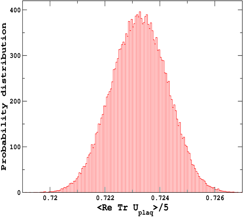
Figure 7: The probability distribution of $\langle{\rm ReTr}U_{\Box}\rangle/5$ for $SU(5)$ gauge theory in a volume $40^{2}\times 3$ at gauge coupling $\beta=32.0513$, close to criticality. For a normal strength first order transition, one expects two well-separated peaks.

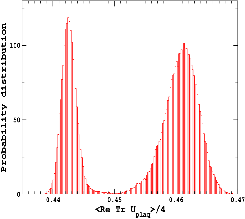
Figure 8: The probability distribution of $\langle{\rm ReTr}U_{\Box}\rangle/4$ for $Sp(2)$ gauge theory in a volume $20^{3}\times 2$ at gauge coupling $\beta=6.465$, close to criticality. There are two clearly indentifiable peaks, whose separation indicates a normal strength first order deconfinement transition.

4 Discussion

As we stated at the outset, a first order deconfinement transition was expected in $(2+1)$-dimensional $SU(5)$ gauge theory and we found no surprises. The fact that the transition appears to be weak, as measured by the latent heat, might even have been suggested by the very large correlation length $\xi$ in the 2-dimensional $Z(5)$ Potts model at the critical point. However, the effective action for the Polyakov loop has a complicated non-local form. That it shares the dimensionality and global symmetry of the Potts model does not dictate its functional form and ultimately the behavior of the deconfinement transition. It was very unlikely to discover a new universality class for the phase transition of the gauge theory, but since lattice simulations can give a definitive answer, we believe we have ruled out this possibility.

Although is seems clear that the first order transition of $SU(N)$ gauge theory increases in strength with $N$, it has been suggested that the $N\rightarrow\infty$ transition might be of second order [25]. Then the weak first order transition for $N=3$ in $(3+1)$ dimensions would be a small perturbation around the large-$N$ limit, consistent with everything else known about QCD phenomenology using the $1/N$ expansion. This might be an attractive scenario, but it is completely opposed by all the evidence.

The general picture appears consistent: where universality classes are available for “small” gauge groups, the deconfinement transition is of second order and has the universal properties of the ordering transition of the respective spin model. However the transition switches to being first order as the gauge group increases in size, both in $(2+1)$ and $(3+1)$ dimensions, even though there are available universality classes. It is even more surprising that $(3+1)$-dimensional $G(2)$ gauge theory has a first order transition, given that the center is trivial. It is easy to correlate this general behavior with the size of the gauge groups and speculate that the large number of degrees of freedom is the driving force. One hopes that this collection of information can give some insight into the full behavior of the Polyakov loop effective action or other properties of the gauge theory.

5 Acknowledgements

We would like to thank Michele Pepe for very helpful discussions and Urs Wenger for the use of his invaluable code to perform the reweighting of the ensembles. This work was supported by the U.S. Department of Energy under the grant DOE-FG03-97ER40546.

$\beta$	$\langle{\rm ReTr}U_{\Box}\rangle/5$
2.0	0.04001(3)
4.0	0.08020(3)
6.0	0.12104(3)
8.0	0.16318(3)
10.0	0.20737(3)
12.0	0.25432(4)
14.0	0.30504(4)
16.0	0.36066(6)
18.0	0.42270(7)
20.0	0.48971(8)
22.0	0.55268(7)
24.0	0.60331(6)
26.0	0.64261(5)
28.0	0.67409(5)
30.0	0.70005(4)
32.0	0.72189(4)
34.0	0.74076(4)
36.0	0.75704(4)
38.0	0.77142(3)
40.0	0.78411(2)
42.0	0.79546(2)
44.0	0.80564(2)
46.0	0.81478(2)
48.0	0.82313(2)
50.0	0.83074(2)
52.0	0.83773(2)
54.0	0.84409(2)
56.0	0.85002(2)
58.0	0.85549(2)
60.0	0.86057(2)

Table 1: The plaquette expectation values $\langle{\rm ReTr}U_{\Box}\rangle/5$ as a function of the bare gauge coupling $\beta=10/g^{2}$ in $6^{3}$ volumes. The errors are in parentheses.

$L_{t}$	$\beta_{c,\infty}$	$(\chi_{\rm max}/L^{2})_{\infty}$
3	32.0765(54)	0.00854(11)
4	41.113(12)	0.00685(13)
5	50.275(20)	0.00641(25)

Table 2: The critical gauge coupling and rescaled peak susceptibility for $L_{t}=3,4$ and 5, extrapolated to the infinite-volume limit. The estimated errors are in parentheses.

$L$	$\Delta$
16	0.00130(10)
18	0.00119(8)
22	0.00118(5)
28	0.00113(6)
34	0.00108(8)
40	0.00107(5)

Table 3: The latent heat $\Delta$ at the critical temperature for $L_{t}=3$. The estimated errors, in parentheses, include the ambiguity in identifying which gauge configurations are in the confined and deconfined phase.

References

- [1] G. ’t Hooft, Nucl. Phys. B 72, 461 (1974); E. Witten, Nucl. Phys. B 160, 57 (1979).
- [2] A. V. Manohar, arXiv:hep-ph/9802419.
- [3] K. J. Juge, J. Kuti and C. Morningstar, Phys. Rev. Lett. 90, 161601 (2003).
- [4] M. Engelhardt, arXiv:hep-lat/0509021.
- [5] G. ’t Hooft, Nucl. Phys. B 138, 1 (1978), Nucl. Phys. B 153, 141 (1979); K. Holland and U. J. Wiese, arXiv:hep-ph/0011193.
- [6] B. Svetitsky and L. G. Yaffe, Nucl. Phys. B 210, 423 (1982).
- [7] J. Kuti, J. Polonyi and K. Szlachanyi, Phys. Lett. B 98, 199 (1981); L. D. McLerran and B. Svetitsky, Phys. Rev. D 24, 450 (1981), Phys. Lett. B 98, 195 (1981); J. Engels, F. Karsch, H. Satz and I. Montvay, Phys. Lett. B 101, 89 (1981); R. V. Gavai, Nucl. Phys. B 215, 458 (1983); R. V. Gavai, F. Karsch and H. Satz, Nucl. Phys. B 220, 223 (1983).
- [8] J. Engels, J. Fingberg and M. Weber, Nucl. Phys. B 332, 737 (1990); J. Engels, J. Fingberg and D. E. Miller, Nucl. Phys. B 387, 501 (1992).
- [9] T. Celik, J. Engels and H. Satz, Phys. Lett. B 125, 411 (1983); J. B. Kogut, M. Stone, H. W. Wyld, W. R. Gibbs, J. Shigemitsu, S. H. Shenker and D. K. Sinclair, Phys. Rev. Lett. 50, 393 (1983); S. A. Gottlieb, J. Kuti, D. Toussaint, A. D. Kennedy, S. Meyer, B. J. Pendleton and R. L. Sugar, Phys. Rev. Lett. 55, 1958 (1985); F. R. Brown, N. H. Christ, Y. F. Deng, M. S. Gao and T. J. Woch, Phys. Rev. Lett. 61 (1988) 2058; M. Fukugita, M. Okawa and A. Ukawa, Phys. Rev. Lett. 63, 1768 (1989); N. A. Alves, B. A. Berg and S. Sanielevici, Phys. Rev. Lett. 64, 3107 (1990).
- [10] B. Lucini, M. Teper and U. Wenger, Phys. Lett. B 545, 197 (2002), JHEP 0401, 061 (2004), JHEP 0502, 033 (2005).
- [11] M. Teper, Phys. Lett. B 313, 417 (1993); J. Engels, F. Karsch, E. Laermann, C. Legeland, M. Lutgemeier, B. Petersson and T. Scheideler, Nucl. Phys. Proc. Suppl. 53, 420 (1997); J. Christensen, G. Thorleifsson, P. H. Damgaard and J. F. Wheater, Phys. Lett. B 276, 472 (1992), Nucl. Phys. B 374, 225 (1992).
- [12] M. Gross and J. F. Wheater, Z. Phys. C 28, 471 (1985); P. de Forcrand and O. Jahn, Nucl. Phys. Proc. Suppl. 129, 709 (2004).
- [13] K. Holland, M. Pepe and U. J. Wiese, Nucl. Phys. B 694, 35 (2004), Nucl. Phys. Proc. Suppl. 129, 712 (2004), arXiv:hep-lat/0309008.
- [14] J. Hove and A. Sudbo, Phys. Rev. E, 046107 (2003), arXiv:cond-mat/0301499.
- [15] K. Holland, P. Minkowski, M. Pepe and U. J. Wiese, Nucl. Phys. B 668, 207 (2003), Nucl. Phys. Proc. Suppl. 119, 652 (2003).
- [16] Michele Pepe, private communication.
- [17] F. Y. Wu, Rev. Mod. Phys. 54, 235 (1982).
- [18] A. Klümper, A. Schadscheider and J. Zittartz, Z. Phys. B76, 247 (1989); E. Buffenoir and S. Wallon, J. Phys. A26, 3045 (1993); C. Borgs and W. Janke, J. Phys. I (France) 2, 649 (1992).
- [19] This work is referred to in M. Teper, arXiv:hep-lat/0509019.
- [20] A. M. Polyakov, Phys. Lett. B 72, 477 (1978); L. Susskind, Phys. Rev. D 20, 2610 (1979).
- [21] M. Creutz, Phys. Rev. D 21, 2308 (1980).
- [22] S. L. Adler, Phys. Rev. D 23, 2901 (1981), Phys. Rev. D 37, 458 (1988); M. Creutz, Phys. Rev. D 36, 515 (1987); F. R. Brown and T. J. Woch, Phys. Rev. Lett. 58, 2394 (1987).
- [23] N. Cabibbo and E. Marinari, Phys. Lett. B 119, 387 (1982).
- [24] A. M. Ferrenberg and R. H. Swendsen, Phys. Rev. Lett. 63, 1195 (1989), Phys. Rev. Lett. 61, 2635 (1988); M. Falcioni, E. Marinari, M. L. Paciello, G. Parisi and B. Taglienti, Phys. Lett. B 108, 331 (1982).
- [25] R. D. Pisarski and M. Tytgat, arXiv:hep-ph/9702340, arXiv:hep-ph/0203271.