Pion form factor with chirally improved fermions

Abstract:

We present results for Monte Carlo calculations of the electromagnetic vector and scalar form factors of the pion in a quenched simulation. We work at a lattice spacing of 0.15 fm and use two lattice volumes up to a spatial size of 2.4 fm. The pion form factors in the space-like region are determined for pion masses down to 340 MeV.

PoS(LAT2005)126

1 Introduction

We present a first-principles calculation of off-forward matrix elements of operators that measure the vector and scalar form factors of the pion, utilizing chirally improved fermions [1, 2]. The vector form factor $F_{\pi}$ is defined by

$$\langle\pi^{+}(\mathbf{p}_{f})|\,V_{\mu}\,|\pi^{+}(\mathbf{p}_{i})\rangle_{\textrm{\scriptsize cont}}=(p_{f}+p_{i})_{\mu}\,F_{\pi}(Q^{2})\;,$$ (1)

where $Q^{2}=(p_{f}-p_{i})^{2}$ is the space-like invariant momentum transfer squared, and $V_{\mu}=2/3\;\overline{u}\,\gamma_{\mu}\,u-1/3\;\overline{d}\,\gamma_{\mu}\,d$ is the vector current. Electromagnetic gauge invariance implies the constraint $F_{\pi}(0)=1$. The mean square charge radius is defined as

$$\langle r^{2}\rangle_{\textrm{\scriptsize v}}=-6\,\frac{d}{dQ^{2}}\,F_{\pi}(Q^{2})\Big{|}_{Q^{2}=0}\;.$$ (2)

The scalar form factor $\Gamma_{\pi}$ is given by the matrix element of the scalar operator

$$\langle\pi^{+}(\mathbf{p}_{f})|\,m_{u}\,\overline{u}\,u+m_{d}\,\overline{d}\,d\,|\pi^{+}(\mathbf{p}_{i})\rangle=\Gamma_{\pi}(Q^{2})\;.$$ (3)

From chiral perturbation theory one knows that the scalar form factor at $Q^{2}=0$ is the so-called sigma term which behaves like $\Gamma_{\pi}(0)\sim M_{\pi}^{2}$ near zero momentum transfer. The scalar radius $\langle r^{2}\rangle_{s}$ can be obtained from

$$\frac{\Gamma_{\pi}(Q^{2})}{\Gamma_{\pi}(0)}=1-\frac{1}{6}\,\langle r^{2}\rangle_{s}\,Q^{2}+{\cal O}\big{(}Q^{4}\big{)}\;.$$ (4)

For a detailed discussion of chiral perturbation theory in this context see [3].

2 Strategy

In order to compute the form factors, we need to evaluate off-forward matrix elements (at several transferred momenta), i.e., the expectation values of

$${\mathrm{Tr}}\,\left(\sum_{\mathbf{y};y_{0}=\tau}\,e^{i\,\mathbf{q}\cdot\mathbf{y}}\,S(0,y)\;O\;\sum_{\mathbf{x};x_{0}=t}\,e^{-i\,\mathbf{p}\cdot\mathbf{x}}\,S(y,x)\,\gamma_{5}\,S(x,0)\,\gamma_{5}\right)\;,$$ (5)

where $S(y,x)$ is the quark propagator from $x$ to $y$ and $O$ denotes the operator inserted at $y$. We use the notation $\mathbf{p}\equiv\mathbf{p}_{f}$, $\mathbf{r}\equiv\mathbf{p}_{i}$ and momentum transfer $\mathbf{q}=\mathbf{p}-\mathbf{r}$. These matrix elements have been evaluated by using the sequential source method where the sequential propagator can be easily computed by an additional inversion of the Dirac operator for each choice of the final momentum.

We extract physical matrix elements by computing ratios of 3-point and 2-point correlators:

$$R(t,\tau;\mathbf{p},\mathbf{q})=\frac{\langle P(t;\mathbf{p})\,O(\tau;\mathbf{q})\,\overline{P}(0;\mathbf{r})\rangle}{\langle P(t;\mathbf{p})\,\overline{P}(0;\mathbf{p})\rangle}\,\sqrt{\,\frac{\langle P(t;\mathbf{p})\,\overline{P}(0;\mathbf{p})\rangle\,\langle P(\tau;\mathbf{p})\,\overline{P}(0;\mathbf{p})\rangle\,\langle P(t-\tau;\mathbf{r})\,\overline{P}(0;\mathbf{r})\rangle}{\langle P(t;\mathbf{r})\,\overline{P}(0;\mathbf{r})\rangle\,\langle P(\tau;\mathbf{r})\,\overline{P}(0;\mathbf{r})\rangle\,\langle P(t-\tau;\mathbf{p})\,\overline{P}(0;\mathbf{p})\rangle}}\;,$$ (6)

where $P$ denotes the pseudoscalar interpolator. We keep the sink fixed at time $t$ and change the timeslice $\tau$ where the operator $O$ sits (scanning a range of timeslices). $R(t,\tau;\mathbf{p},\mathbf{q})$ should exhibit two plateaus in $\tau$, for $0\ll\tau\ll t$ and $t\ll\tau\ll T$. Note that the terms under the square root become trivial for $\mathbf{q}=(0,0,0)$.

$16^{3}\times 32$	0.74 GeV	1.04 GeV	1.28 GeV	1.48 GeV
$12^{3}\times 24$	0.98 GeV	1.39 GeV	1.71 GeV	1.97 GeV

Table 1: Values of the nonzero momentum transfers.

We choose for initial and final momenta $|\mathbf{p}_{f}|=|\mathbf{p}_{i}|$ such that $E_{f}=E_{i}$ and the transferred 4-momentum is given by $Q^{2}=|\mathbf{q}|^{2}$. In this way one achieves for the electromagnetic form factor [4] the cancellation of the kinematical factors in (1) and

$$\langle\pi(\mathbf{p}_{f})|V_{\mu}|\pi(\mathbf{p}_{i})\rangle_{\textrm{\scriptsize latt}}=\frac{1}{2\,\sqrt{E_{f}E_{i}}}\langle\pi(\mathbf{p}_{f})|V_{\mu}|\pi(\mathbf{p}_{i})\rangle_{\textrm{\scriptsize cont}}\;.$$ (7)

Indeed, with this choice of momenta, and using the $\mu=4$ component of the vector current, the overall factor becomes

$$\frac{E_{f}+E_{i}}{2\sqrt{E_{f}E_{i}}}=1.$$ (8)

This cancellation is unfortunately no longer possible in the calculation of the scalar form factor, where a remaining multiplication by the quantity $2\,\sqrt{E_{f}\,E_{i}}$ is still needed.

We have made the choice $|\mathbf{p}_{f}|=|\mathbf{p}_{i}|=\sqrt{2}\,p_{0}$, where $p_{0}=2\,\pi/(a\,L)$ denotes the smallest (spatial) momentum unit. Fixing the final (sink) momentum to $\mathbf{p}_{f}=(1,1,0)\,p_{0}$, we get twelve values for the initial momentum. They give rise to four nonzero (and equidistant) values for the momentum transfer, $Q^{2}=2\,n\,p_{0}^{2}$ for $n=0,\,1,\,2,\,3,\,4$ (see Table 1). We could also consider larger values of the module of the initial momentum. In this case, however, the statistical errors become much larger, and moreover we could not use Eq. (8) anymore. A change of the momentum at the sink would require the expensive computation of a new set of sequential propagators.

In the Monte Carlo simulations additional numerical noise due to the momentum projection of the sink and of the operator onto nonzero momentum transfer $\mathbf{q}$ arises. The 2-point correlators may even become negative (within the statistical errors) on timeslices near the symmetry point. A reasonable choice was to put the sink at a timeslice smaller than $T/2$, such that the 2-point functions have smaller errors. In particular, we have put the sink at timeslice $t=8$, while the source sits at timeslice $t=1$.

3 Simulation parameters

We use the chirally improved Dirac operator [1, 2, 5], which constitutes an approximate Ginsparg-Wilson operator. The gauge action is the Lüscher-Weisz tadpole improved action at $\beta=7.9$, corresponding to a lattice spacing of 0.148 fm (determined from the Sommer parameter). Although we expect improved scaling properties, here we do not study scaling behavior. The hadron interpolators are constructed from Jacobi-smeared quark sources and sinks.

We have done simulations using two volumes, $12^{3}\times 24$ (200 configurations for each mass) and $16^{3}\times 32$ (100 configurations for each mass). This corresponds to spatial lattice sizes of $a\,L\sim 1.8\;$fm and $a\,L\sim 2.4\;$fm respectively.

We work at several values of the bare quark mass; the corresponding meson masses are given in Table 2. The jackknife method is used for estimating the statistical errors of our results.

	$16^{3}\times 32$	$16^{3}\times 32$	$16^{3}\times 32$	$12^{3}\times 24$	$12^{3}\times 24$
$m$	0.02 $a^{-1}$	0.04 $a^{-1}$	0.06 $a^{-1}$	0.04 $a^{-1}$	0.06 $a^{-1}$
$m_{\pi}$	342 MeV	471 MeV	571 MeV	474 MeV	575 MeV
$m_{\rho}$	845 MeV	895 MeV	941 MeV	952 MeV	976 MeV

Table 2: Pion and rho masses at the various quark masses simulated [5].

4 Results

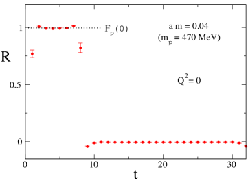
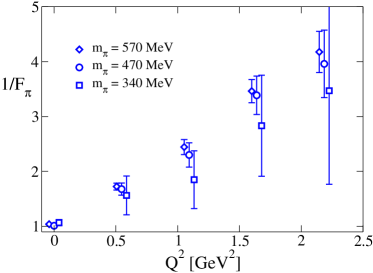
Figure 1: (a) L.h.s.: The ratio $R(t,\tau;\mathbf{p},\mathbf{q})$ leading to the electromagnetic vector form factor at zero momentum transfer, for the $16^{3}\times 32$ lattice at $m_{\pi}=470$ MeV. (b) R.h.s.: The inverse vector form factor for the three available masses on the $16^{3}\times 32$ lattice. For presentation purposes the data points for different masses are slightly shifted horizontally.

In Fig. 1a we show an example for the observed plateau behavior of the ratio (6). Fitting the central points of the plateau then provides values for the electromagnetic form factor of the pion.

When comparing the results to physical, renormalized quantities we have to multiply with renormalization factors relating the raw results to the $\overline{\textrm{MS}}$-scheme. For the chirally improved Dirac operator these have been determined in [6] and all results we show are already converted to the $\overline{\textrm{MS}}$-scheme. Although the vector current is pointlike and not conserved, the value $Z_{V}=0.9586(2)$ turns out to be close to unity. The resulting $F_{\pi}(0)$ is not constrained to unit value, but comes very close as may be seen, e.g., in Fig. 1a. This fact is also obvious from Fig. 1b, where we plot the inverse of the vector form factor determined for all the momentum transfer values and quark masses studied on the $16^{3}\times 32$ lattice.

The electromagnetic pion form factor in the time-like region is dominated by the $\rho$-meson. In the space-like region it may therefore be well approximated by a monopole form, $F_{\pi}(Q^{2})={m_{V}^{2}}/({m_{V}^{2}+Q^{2}})$, such that $1/F_{\pi}$ has the linear behavior indeed observed in Fig. 1b. In that approximation the mean square radius is $6/m_{V}^{2}$.

As the vector meson dominance (VMD) model is just an approximation one expects corrections due to other resonances and more-particle channels in the time-like region. These may be taken into account by additional pole terms. The data (cf. Fig. 1b) does not really require such a multi-parameter fit and for the presentation here we discuss only the results of a linear fit.

The derivative of the form factor at $Q^{2}=0$ gives the charge radius, as shown in Fig. 2a. Whereas the large mass results are compatible with a constant, the lowest mass is smaller but with a very large statistical error. The values are quite compatible with values from [4] at comparable quark mass values. A fit to a constant gives $\langle r^{2}\rangle_{\textrm{\scriptsize v}}=0.279(16)\;\textrm{fm}^{2}$. The current PDG average is $0.45(1)$ [7].

The value of $\langle r^{2}\rangle_{\textrm{\scriptsize v}}$ is in the VMD model inversely proportional to the mass squared of the $\rho$-meson. We obtain $m_{\textrm{\scriptsize VDM}}^{2}=0.83(5)\;\textrm{GeV}^{2}$. This is close to the range of values obtained for $m_{\rho}^{2}$ in the BGR analysis [5] in the direct $\rho$-channel (e.g., $0.80\;\textrm{GeV}^{2}$ at $a\,m=0.04$). These large values for the $m_{\rho}$ mass might at least in part explain (via the VMD model) our low result for $\langle r^{2}\rangle_{\textrm{\scriptsize v}}$.

The scalar form factor also has disconnected contributions which we disregard here (like it is done usually due to the related technical complications). We determine the scalar radius squared from a linear fit to the $Q^{2}$-dependence of the scalar form factor (now explicitely normalized according to Eq. 4). The resulting values, shown in Fig. 2b, are almost an order of magnitude smaller than for the electromagnetic case. We obtain an average for the scalar radius of $\langle r^{2}\rangle_{s}=0.034(6)\;\textrm{fm}^{2}$. It is also smaller than the values expected for full QCD.

In chiral perturbation theory the scalar radius is related to the quark mass dependence of the pion decay constant

$$f_{\pi}/f=1+\frac{1}{6}\,\langle r^{2}\rangle_{s}\,M_{\pi}^{2}+\frac{13\,M_{\pi}^{2}}{192\pi^{2}f_{\pi}^{2}}+{\cal O}\big{(}M_{\pi}^{4})\;,$$ (9)

and in Ref. [3] values around $\langle r^{2}\rangle_{s}\sim 0.55-0.75\;\textrm{fm}^{2}$ were expected. Results for the pion decay constant in a recent full QCD lattice calculation [8] lead to the value $\langle r^{2}\rangle_{s}=0.5\pm 0.1~{}\textrm{fm}^{2}$. A corresponding analysis of the quenched BGR data [9] gives again a small value $0.08-0.13\;\textrm{fm}^{2}$. This seems to imply that $\langle r^{2}\rangle_{s}$ is very sensitive to quenching.

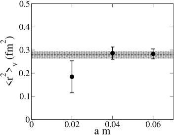
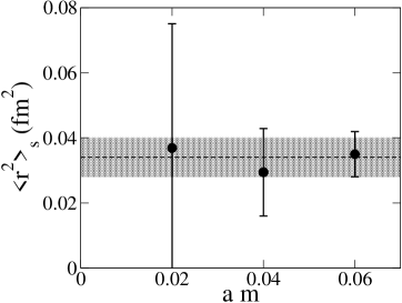
Figure 2: The mean square radius for the three available masses on the $16^{3}\times 32$ lattice for (a) the vector (l.h.s.) and (b) the scalar (r.h.s.) form factor.

5 Conclusions

Chirally improved fermions provide a valid framework for a first principles lattice study of the hadron structure. They are Ginsparg-Wilson-like fermions and less expensive than other types of chiral fermions. We have begun the study of hadron structure by investigating the form factors of the pion. The vector form factor is consistent with expectations in its general form, although the charge radius is 40% smaller than in experiment. For the scalar form factor the scalar radius is much lower than one would expect from unquenched calculations. Both effects may be signals of quenching.

Further progress could be achieved - as usual - by using better statistics, more momenta, and larger lattices, both in lattice units (to study finite volume effects) and in physical units (to access lower transferred momenta).

Most computations were done on the Hitachi SR8000-F1 at the Leibniz Rechenzentrum in Munich, and we thank the staff for support.

References

- [1] C. Gattringer, A new approach to Ginsparg-Wilson fermions, Phys. Rev. D 63 (2001) 114501 [hep-lat/0003005].
- [2] C. Gattringer, I. Hip, and C. B. Lang, Approximate Ginsparg-Wilson fermions: A first test, Nucl. Phys. B 597 (2001) 451 [hep-lat/0007042].
- [3] B. Ananthanarayan, I. Caprini, G. Colangelo, J. Gasser, and H. Leutwyler, Scalar form factors of light mesons, Phys. Lett. B 602 (2004) 218 [hep-ph/0409222].
- [4] J. van der Heide, J. Koch, and E. Laermann, Pion structure from improved lattice QCD: form factor and charge radius at low masses, Phys. Rev. D 69 (2004) 094511 [hep-lat/0312023].
- [5] C. Gattringer, M. Göckeler, P. Hasenfratz, et. al., Quenched spectroscopy with fixed-point and chirally improved fermions, Nucl. Phys. B 677 (2004) 3 [hep-lat/0307013].
- [6] C. Gattringer, M. Göckeler, P. Huber, and C. B. Lang, Renormalization of bilinear quark operators for the chirally improved lattice Dirac operator, Nucl. Phys. B 694 (2004) 179 [hep-lat/0404006].
- [7] S. Eidelman, et al., Review of Particle Physics, Phys. Lett. B 592 (2004) 1.
- [8] C. Aubin, C. Bernard, C. DeTar, et al., Light pseudoscalar decay constants, quark masses, and low energy constants from three-flavor lattice QCD, Phys. Rev. D 70 (2004) 114501 [hep-lat/0407028].
- [9] C. Gattringer, P. Huber, and C. B. Lang, Lattice calculation of low energy constants with Ginsparg-Wilson type fermions (2005) [hep-lat/0509003].