Light hadron and diquark spectroscopy in quenched QCD
with overlap quarks on a large lattice

Abstract

A simulation of quenched QCD with the overlap Dirac operator has been completed using 100 Wilson gauge configurations at $\beta=6$ on an $18^{3}\times 64$ lattice and at $\beta=5.85$ on a $14^{3}\times 48$ lattice, both in Landau gauge. We present results for light meson and baryon masses, meson final state “wave functions,” and other observables, as well as some details on the numerical techniques that were used. Our results indicate that scaling violations, if any, are small. We also present an analysis of diquark correlations using the quark propagators generated in our simulation.

I Introduction

Preserving chiral symmetry presented a notorious difficulty for the early formulations of lattice Quantum Chromodynamics (QCD). The problem stemmed from the fact that an ultralocal discretization of the Dirac equation must either abandon full chiral symmetry or introduce extra fermionic degrees of freedom (doublers), with associated no-go theorems for lattice fermions Karsten and Smit (1981); Nielsen and Ninomiya (1981). It was only about a decade ago that seminal work by Kaplan, Shamir, Neuberger, Narayanan, and others provided a way out of the impasse, through the introduction of domain-wall Kaplan (1992); Shamir (1993) and overlap Narayanan and Neuberger (1995a); Narayanan and Neuberger (1994); Neuberger (1998a) formulations of lattice fermions. These two closely related discretizations of the Dirac equation avoid the no-go theorems by forfeiting ultralocality, while retaining locality, and satisfy an identity, the Ginsparg-Wilson relation Ginsparg and Wilson (1982a), which allows one to extend to the lattice the chiral symmetry of continuum QCD Lüscher (1998). Unfortunately, the satisfactory properties of the new lattice formulations come with a heavy computational cost, since they entail either extension of the lattice in a fifth dimension or very demanding large matrix manipulations. It is therefore important to subject these novel discretizations to the test of lattice QCD simulations on systems of realistically large size, in order to explore the adequacy of the necessary numerical techniques and to validate the good properties that are expected to follow from the preservation of chiral symmetry. In this paper, we present the results of such an investigation, where we used the overlap Dirac operator to simulate quenched QCD on two lattices, of size $18^{3}\times 64$ and $14^{3}\times 48$.

One early simulation of quenched QCD with overlap quarks was performed in Giusti et al. (2001, 2002). Pioneering investigations of QCD with the overlap fermion discretization were also presented in Edwards et al. (1999a); Hernández et al. (1999a); DeGrand (2001); Liu et al. (2001); Hernández et al. (2001, 2002); Chiu et al. (2002); Garron et al. (2004); Mathur et al. (2005); Chen et al. (2004); Chiu and Hsieh (2003); DeGrand (2004). In the work of Giusti et al. (2001, 2002), quenched QCD was simulated with the Wilson gauge action at $\beta=6$ on a lattice of size $16^{3}\times 32$. An expansion into fractions, after projection of a small number of low lying eigenvectors, was used to calculate the overlap Dirac operator. It was shown that the available computational methods could produce accurate results for the quark propagators in a reasonable amount of time with moderately powerful computer resources (capable of 10 to 20 Gflops sustained). Satisfactory results were obtained on the pseudoscalar spectrum, strange quark mass, quark condensate, renormalization constants, and a few other observables, and the good chiral behavior of the theory was verified. It also became apparent, however, that the extent of the lattice in the temporal direction was too small for a meaningful calculation of other parameters of the hadron spectrum, such as vector meson and baryon masses, as well as for a reliable estimate of important matrix elements. We decided therefore to extend the scope of the investigation by considering a bigger lattice, with a time extent twice as large. The spatial extent was also slightly increased, with the final choice of lattice size, $18^{3}\times 64$, motivated by a careful assessment of the computer resources we could rely upon. After completing the calculation of the quark propagators on the $18^{3}\times 64$ lattice, we also simulated a system of size $14^{3}\times 48$, with correspondingly coarser lattice spacing, in order to check scaling.

For the calculations described in this paper we simulated quenched QCD with Wilson gauge action at $\beta=6$ on the $18^{3}\times 64$ lattice and $\beta=5.85$ on the $14^{3}\times 48$ lattice. The corresponding values of the lattice spacing are $a^{-1}=2.12\,{\rm GeV}$ and $a^{-1}=1.61\,{\rm GeV}$, on the basis of the Sommer scale defined by $r_{0}^{2}F(r_{0})=1.65$, $r_{0}=0.5\,{\rm fm}$ Guagnelli et al. (1998); Necco and Sommer (2002). (The determination of $a^{-1}$ from the Sommer scale in quenched QCD is quite accurate and we can consider the corresponding statistical error negligible with respect to the other statistical errors in this work.) Thus, the two lattices are of approximately the same physical volume. For both lattices, we generated 100 gauge configurations using the multihit Metropolis algorithm, with 11,000 lattice upgrades for equilibration and 10,000 lattice upgrades between subsequent configurations. For each configuration, we performed a gauge transformation to Landau gauge. We then calculated the quark propagators with source at the origin and all 12 source color-spin combinations for bare quark mass

$$am\in\{0.03,0.04,0.06,0.08,0.1,0.25,0.5,0.75\}$$ (1)

on the finer $18^{3}\times 64$ lattice, and

$$am\in\{0.03,0.04,0.053,0.08,0.106,0.132,0.33,0.66,0.99\}$$ (2)

on the coarser $14^{3}\times 48$ lattice. The calculation of the quark propagators was done with a conjugate-gradient multimass solver. Technical details of our calculation, as well as relevant formulae, are presented in Appendix A. We should mention here, however, some computational considerations which informed the choices we had to make for our investigation.

The limitations of the quenched approximation are well-known, and forefront calculations today tend to incorporate dynamical quarks. A simulation with dynamical overlap quarks on a lattice similar to the one we studied would have required, however, computational resources at least two orders of magnitude larger than we had available. Moreover, an efficient calculation of quark propagators with the overlap Dirac operator is a necessary prerequisite for overlap simulations with dynamical quarks. We concluded that a quenched calculation would be the best option at present, in that it would allow us to consider a reasonably large lattice and separate the computational problems associated with the calculation of the overlap operator from those of the dynamical fermion feedback. An alternative would have been to perform mixed action calculations, i.e. to use overlap valence quarks in the background of gauge configurations generated with some other type of dynamical quarks, for example those made available by the MILC collaboration (see http://qcd.nersc.gov). While that might have been computationally feasible and may be a good strategy for future calculations, we decided not to proceed in that manner at this stage in order to avoid the entanglement of two different sets of computational effects as well as for a more technical reason, on which we shall now elaborate.

The overlap Dirac operator for a massless quark is given by

$$D=\,\frac{\rho}{a}\,\left(1+\gamma_{5}H(\rho)\,\frac{1}{\sqrt{H(\rho)^{2}}}\,\right)\;,$$ (3)

where $H(\rho)$ stands for the Hermitian Wilson-Dirac operator with mass $-\rho/a$, namely

$$H(\rho) = \gamma_{5}D_{W}(\rho)$$ (4)

$$= \,\frac{\gamma_{5}}{2}\,\sum_{\mu}[\gamma_{\mu}(\nabla_{\mu}-\nabla_{\mu}^{\dagger})+a\nabla_{\mu}^{\dagger}\nabla_{\mu}]-\,\frac{\rho\gamma_{5}}{a}\,$$

with the forward lattice covariant derivative implicitly defined by

$$\nabla_{\mu}\psi(x)=\,\frac{1}{a}\,[U_{\mu}(x)\psi(x+a\hat{\mu})-\psi(x)]\;.$$ (5)

In terms of $D$, the overlap Dirac operator for a quark of mass $m$ is then given by $[1-(am)/(2\rho)]D+m$. (See Appendix A for more details on the overlap Dirac operator.)

In the calculation of the quark propagators, which is based on a conjugate-gradient iterative procedure, at each step one must apply the overlap operator to the current iterate. Equation (3) shows that this requires evaluating the action of $(H^{2})^{-1/2}$ on a quark field, for which in turn one must use some suitable approximation to the inverse square root. Implementing such an approximation, with the required degree of numerical accuracy, becomes more and more demanding the larger the condition number of $H^{2}$, i.e. the larger the value of the ratio between its largest and smallest eigenvalues. Since the largest eigenvalue of $H^{2}$ is bounded, in practice the condition number of the matrix depends on its lowest eigenvalue, or, equivalently, on the gap in the eigenvalues of $H$ around 0. This gap in turn depends on the parameter $\rho$ (which must be carefully chosen) as well as, loosely speaking, on the “amount of disorder” of the gauge configuration. This became quite apparent in our study, where the calculation of the quark propagators on the smaller $14^{3}\times 48$ lattice turned out to be computationally more challenging than the calculation on the $18^{3}\times 64$ lattice, because of the increased “roughness” of the background gauge configurations at the smaller value of $\beta$. A similar dependence is encountered in the domain-wall formulation, where the so called “residual mass,” which measures the deviation from chiral symmetry induced by the truncation in the fifth dimension, is seen to depend on the smoothness of the gauge configuration Blum et al. (2004). Given the fact that the gap in the eigenvalues of $H$ can be substantially affected by the choice of action and by the presence or absence of dynamical fermions, we thought that it would be useful to establish a benchmark by performing a quenched simulation with the most traditional action, namely the Wilson gauge action. We thought that demonstrating that the overlap formulation is amenable to precise calculations on large lattices in this context would be an important step toward the use of more elaborate gauge actions and/or mixed action calculations.

Another choice we had to make concerned the type of quark sources to use. Calculations of the lowest masses in the hadron spectrum are made more precise by the use of extended sources. However, we also wanted to take advantage of our quark propagators for the study of non-perturbative renormalization and the evaluation of selected matrix elements, both of which required point-like sources. Since the high cost of evaluating overlap quark propagators made it impossible for us to use both source terms, we had to adopt point-like sources. Of course, this did not prevent us from using extended sink operators, and indeed some of the results we present here have been obtained with extended sinks. Finally, the non-perturbative renormalization techniques required that the gauge field be brought to Landau gauge prior to evaluating the propagators. We have implemented this gauge fixing for all our gauge configurations (of course, after they have been generated), an additional advantage being that this allowed us to calculate quark-antiquark correlation functions in the final state as well as diquark propagators.

Novel results with respect to the calculations presented in Giusti et al. (2001, 2002) have been obtained for the vector meson spectrum and decay constants, for the baryon spectrum, for correlations among quarks and antiquarks in the final state (which we will refer to as final state “wave functions”), scaling, quark and diquark propagators, non-perturbative renormalization, and meson matrix elements of selected four-quark operators. In this paper, we present our results for the meson spectrum and decay constants, meson final state wave functions, the baryon spectrum, scaling from $\beta=5.85$ to $\beta=6$, and quark and diquark propagators. We will present our results for renormalization constants and matrix elements in a companion paper. We hope to present a more detailed analysis of heavy quark states, as well as a study of diquark correlations within baryons, in future publications.

In Section II, we present our results for light meson observables on the finer $18^{3}\times 64$ lattice. We follow in Section III with our results for the coarser $14^{3}\times 48$ lattice, as well as a scaling comparison between the two lattices. As discussed in Appendix A, we chose $\rho=1.4$ at $\beta=6.0$ and $\rho=1.6$ at $\beta=5.85$ Hernández et al. (1999b, a) so as to optimize the locality properties of our overlap operator. That choice induces a lattice spacing dependence which would have to be parameterized in order to allow for a continuum extrapolation. Since our goal is only an estimate of possible discretization errors, we do not pursue such an approach here. In Section IV, we present our results for the baryon spectrum on the $18^{3}\times 64$ lattice as well as scaling between the two lattices. Finally, in Section V, we present our analysis of diquark correlation functions and diquark spectra. In the Appendices, we give background information on the overlap Dirac operator, present details of our simulation techniques, and present data tables for meson and baryon spectra and other observables.

II Light Meson Observables on the $18^{3}\times 64$ Lattice

II.1 Correlators

We evaluated meson correlators for point source, point sink operators, as well as point source, extended sink operators. As explained in the introduction, computational limitations did not allow us to calculate correlators with extended sources.

We first consider correlators with point sink operators. We only consider connected diagrams, so without loss of generality we take quark and antiquark of different flavors $f_{1}$ and $f_{2}$. The zero-momentum meson correlator is given by

$$G_{AB}(t)=\langle\,\sum_{\vec{x}}\mathrm{Tr}\left[S^{f_{2}}(0;\vec{x},t)\,\Gamma_{A}\gamma_{5}\,(S^{f_{1}}(0;\vec{x},t))^{\dagger}\,\gamma_{5}\Gamma_{B}\right]\rangle\;,$$ (6)

where $S(0;\vec{x},t)$ is the Euclidean quark propagator and $\Gamma_{A}$ and $\Gamma_{B}$ are the Dirac $\gamma$-matrix combinations associated with the meson states $A$ and $B$. An example of such a meson correlator is shown in Fig. 1.

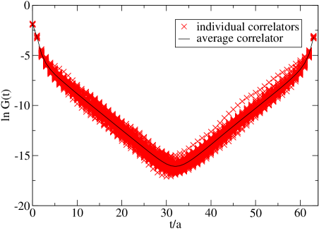
Figure 1: Time dependence of a $PP$ correlator, for quark masses $am_{1}=0.08$, $am_{2}=0.10$.

To obtain ground state meson masses, the zero-momentum meson correlators, which are even under time-reversal, were fit in an appropriate fitting window to the usual functional form

$$G(t)=\,\frac{Z}{M}\,\,e^{-MT/2}\cosh\left[M\left(\,\frac{T}{2}\,-t\right)\right]\;,$$ (7)

where $M$ is the meson mass and $T$ is the extent of the lattice in time, and where we will refer to $Z$ as the correlator matrix element.

For mesons with quarks of non-degenerate mass, we combined the results obtained by an interchange of the two quark masses. In order to increase statistics, we folded the meson correlators over the midpoint $T/2$ and fitted to data below that point. Concerning statistical errors, the data that enter into the fit (the meson correlators at different values of time) are highly correlated, but the amount of data is not sufficient for an evaluation of cross-correlations that would be precise enough for incorporation into the fitting procedure. Thus, we instead used the bootstrap technique. We found that the error estimates became stable when the number of bootstrap samples $n_{B}$ reached a value of approximately 200 and used $n_{B}=300$ in our calculations. We used the bootstrap method for the estimate of the statistical errors in most of the results presented in this paper.

Typically, effective mass plots are used to determine the best fitting window $\{t_{min},t_{max}\}$ for correlators. Examples of such effective mass plots are shown in Fig. 2. Using a cosh fit for the meson correlators allowed a consistent $t_{max}$ of $T/2$. In order to pinpoint the best value for $t_{min}$, we considered scans over different values of $t_{min}$ for a fixed $t_{max}$. An example of such data is shown in Fig. 3. The value of $t_{min}$ chosen was the smallest value (consistent with the errors) before the clear effect of higher states caused the mass prediction to rise. Consideration of the $\chi^{2}$ value from the fit also was used to confirm the choice. If possible, a single value of $t_{min}$ was chosen for all quark mass combinations.

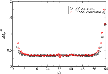
Figure 2: Effective mass plateau for different pseudoscalar correlators at $am=0.08$.

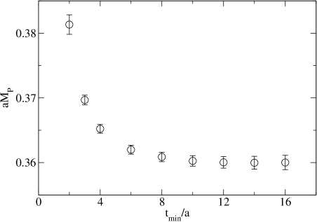
Figure 3: Scanning for optimum $t_{min}$ for $PP$ mass, with $am_{1}=0.08$, $am_{2}=0.10$, and $t_{max}=32$.

II.2 Meson spectra

The effective mass data and fitting window scans in Figs. 2 and 3 suggested use of a fit range $12\leq t/a\leq 32$ in order to extract the pseudoscalar mass. For the vector mass, the fitting range was $8\leq t/a\leq 32$. We illustrate in Fig. 4 our results for the pseudoscalar spectrum for all possible input quark mass combinations. In the quenched approximation, the correlator $G_{PP}(t)$ receives contributions proportional to $1/m^{2}$ and $1/m$ from chiral zero modes that are not suppressed by the fermionic determinant. These unsuppressed contributions, which should vanish in the infinite volume limit, could be sizable at finite volume Hernández et al. (1999a); Blum et al. (2004). A method of handling these quenching artifacts is to consider the difference of pseudoscalar and scalar meson correlators

$$G_{PP-SS}(t)=G_{PP}(t)-G_{SS}(t)\;,$$ (8)

since, by chirality, the quenching artifacts cancel in the difference Blum et al. (2004). The results for the pseudoscalar masses obtained with this correlator are also included in Fig. 4. With our large lattice we do not see any significant difference between the results obtained with $PP$ and $PP-SS$ correlators. Thus, in the remainder of this paper, for what concerns the pseudoscalar masses and matrix elements, we will only consider the $PP$ correlators, except where otherwise noted. For economy of figures, we also show in Fig. 4 the results for correlators with extended sink operators, which will be discussed in section II.4.

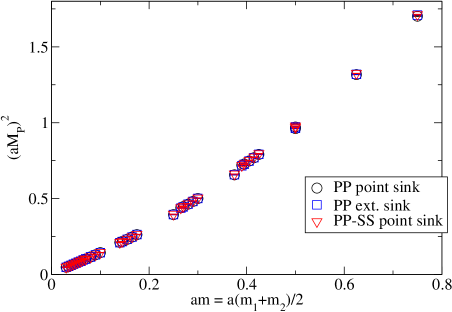
Figure 4: Pseudoscalar meson spectrum for point and extended sinks.

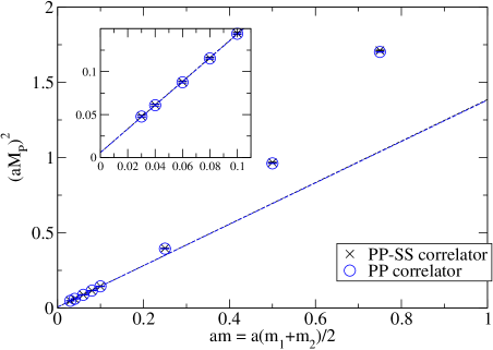
Figure 5: Chiral behavior of meson masses. The solid line corresponds to the best fit to Eq. (9) in the interval $am\leq 0.1$.

The chiral behavior of the pseudoscalar spectrum with degenerate quarks is illustrated in Fig. 5 for the $PP$ and $PP-SS$ correlators. The lightest data point corresponds roughly to a kaon composed of degenerate quarks of mass $am=0.03\sim am_{s}/2$, where $am=a(m_{1}+m_{2})/2$ is the average of the quark and antiquark masses $am_{1}$ and $am_{2}$ in the meson and $am_{s}$ is the bare strange quark mass, all in lattice units. We neglect for the moment the chiral logarithms discussed in Section II.5 and perform a fit to the linear form

$$(aM_{P})^{2}={\cal A}+{\cal B}(am)\;,$$ (9)

where $aM_{P}$ is the pseudoscalar mass. If we fit all data with $am\leq 0.1$ we obtain (see Fig. 5)

$${\cal A}=0.0058(15)\;,\qquad{\cal B}=1.376(15)\qquad$$ (10)

for the $PP$ correlator and

$${\cal A}=0.0059(16)\;,\qquad{\cal B}=1.380(17)\qquad$$ (11)

for the $PP-SS$ correlator. (The corresponding values in Giusti et al. (2001) were ${\cal A}=0.006(4)$, ${\cal B}=1.39(3)$ and ${\cal A}=-0.0005(68)$, ${\cal B}=1.43(7)$ for the $PP$ and $PP-SS$ correlators, respectively.) These results exhibit the good chiral behavior of the overlap formulation. The non-zero value of the intercept $\cal A$ in Eqs. (10) and (11), albeit small, is however statistically significant. Since our results rule out the possibility that this is due to zero modes, the small deviation from chiral behavior can originate either from finite volume effects or chiral logarithms. In a later section we will argue against finite volume effects and show that it is indeed compatible with chiral logs.

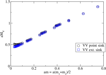
Figure 6: Vector meson spectrum for point and extended sinks.

Using a larger lattice than Giusti et al. (2001) allowed for observation of vector meson states, as shown in Fig. 6, with $aM_{V}$ the vector meson mass. The observation of vector meson states was enhanced by use of extended sink operators, as discussed in Section II.4. Our results for the meson spectrum are reproduced in the tables presented in Appendix B.

II.3 Axial Ward identity and $Z_{A}$

Exact chiral symmetry implies a conserved axial current, and the associated axial Ward identity (AWI) predicts a constant value for the ratio

$$\rho(t)=\,\frac{G_{\nabla_{0}A_{0}P}(t)}{G_{PP}(t)}\,\;.$$ (12)

The conserved axial current is a local, but not ultralocal, operator. The ultralocal axial current

$$A_{0}=\bar{\psi}_{1}(x)\gamma_{0}\gamma_{5}\left[(1-\,\frac{a}{2\rho}\,D)\psi_{2}\right](x)$$ (13)

differs from the exactly conserved axial current by a finite renormalization factor $Z_{A}$ and possible corrections $\mathcal{O}(a^{2})$. We calculated the correlator in Eq. (12) with the current of Eq. (13) and using the lattice central difference for $\nabla_{0}$, corrected so as to take into account the $\rm sinh$ behavior of the correlator. Figure 7 shows the observation of plateaus for all of our quark masses in the range $8\leq t/a\leq 56$.

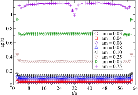
Figure 7: AWI ratio as a function of time for all degenerate quark mass combinations.

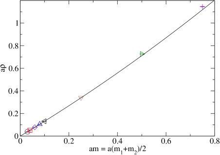
Figure 8: Axial Ward identity fit.

The fit shown in Fig. 8 to

$$a\rho={\cal A}+2(am)/Z_{A}+{\cal C}(am)^{2}$$ (14)

gives

$${\cal A}=0.00002(10)\;,\ \ Z_{A}=1.5555(47)\;,\ \ {\cal C}=0.273(32)\;.$$ (15)

(In Giusti et al. (2001), the results were ${\cal A}=-0.00002(7)$, $Z_{A}=1.555(4)$ and ${\cal C}=0.277(12)$.) The fact that the value of $\mathcal{A}$ is consistent with zero is an excellent indication of the good chiral behavior of overlap fermions (compared to the residual mass found in domain-wall fermion calculations). Also, $\mathcal{C}$ is rather small, a possible indication that discretization errors might be smaller than expected on the basis of purely dimensional arguments.

II.4 Extended sink operators

For some correlators, e.g. the vector $VV$ correlators, the signal for the ground state is small when point sources and point sinks are used. In particular, the use of point sources and sinks causes coupling to excited states that do not decay until relatively large values of $t_{min}$. The signal can be improved by using non-local extended operators instead of local point operators in the representation of the meson Gottlieb (1985). Since, as mentioned in Section I, our quark propagators were calculated using point sources, we were limited only to the case of extended sinks. Here we elaborate on our use of extended sink operators.

We consider the correlator

$$G(r,t) = \sum_{\vec{x},\vec{y}}\left\langle\mathrm{Tr}\left[S^{f_{2}}(0;\vec{x},t)\,\Gamma_{A}\gamma_{5}\,(S^{f_{1}}(0;\vec{y},t))^{\dagger}\,\gamma_{5}\Gamma_{B}\right]\right.$$ (16)

$$\qquad\times\;\left.\delta(|\vec{x}-\vec{y}|-r)\right\rangle\;,$$

where the $\delta$-function is approximated on the lattice with a Kronecker $\delta$, taking into account the multiplicity of the sites. The quantity $r$ is the separation of the quark and antiquark at the sink in lattice units. No gauge transport factor is needed to make the non-local correlator in Eq. (16) well defined because we calculated the quark propagators in Landau gauge.

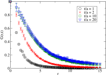
Figure 9: $PP$ extended sink correlators $G(r,t)$ for various $t/a$ and $am_{1}=am_{2}=0.03$.

We calculated $G(r,t)$ for $PP$ and $VV$ correlators. A fast Fourier transform (FFT) was used in order to speed up the calculation; we first Fourier transformed the quark propagators and then used the convolution theorem. That reduced the double summation over spatial lattice sites to a single sum, decreasing the computational time by almost three orders of magnitude Hauswirth (2002). Figure 9 illustrates the average value of the $G(r,t)$ correlators for pseudoscalar mesons with quark mass $am=0.03$, each normalized to unity at $r=0$. A clear ground state “wave function” is apparent after about $t/a=8$.

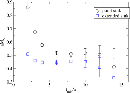
Figure 10: Comparison of $t_{min}$ scans for $VV$ point and extended sinks with $am_{1}=am_{2}=0.03$.

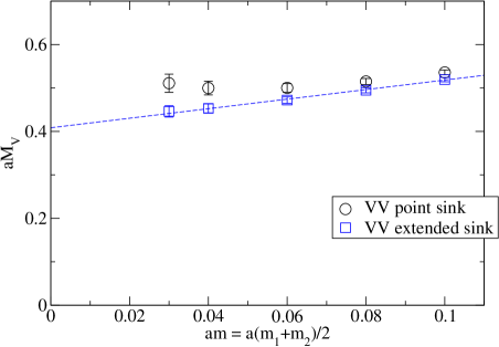
Figure 11: Vector meson spectrum for $am\leq 0.1$.

The observation that the wave function settles into a definite profile representing the contribution of the ground state allows us to use this ground state wave function to construct extended sink correlators. For both the $PP$ and $VV$ correlators, we used the corresponding function $\varphi(r)\equiv G(r,8a)$ (of course, with different $\varphi(r)$ for the pseudoscalar and vector states) to define an extended sink correlator

$$G_{\rm ext}(t)=\sum_{r}\varphi(r)G(r,t)\;,$$ (17)

from which we then extracted the meson mass.

The use of extended sinks was most valuable in the calculation of the vector meson spectrum, due to the resulting increase in the size of the fitting window (see Fig. 10). The point sink and extended sink vector meson spectra are compared in Fig. 11 for low quark mass, $am\leq 0.1$. A linear fit of the quark-mass dependence of the vector meson mass obtained from the extended sink data gives

$$aM_{V}=0.409(15)+1.10(13)\,(am)\;.$$ (18)

We note that the chiral limit value of 0.409(15) is larger than the value 0.366 obtained using the Sommer scale value for the lattice spacing and the experimental $\rho$ mass. As we will discuss in a later section, the discrepancy gives an indication of the systematic error induced by the quenched approximation.

II.5 Quenched chiral logarithms

A linear fit to the pseudoscalar masses for quark mass $am\leq 0.1$ (see Fig. 5) produces a line with an intercept which is very small, but statistically different from zero, indicating a deviation from the chiral behavior $(aM_{P})^{2}\propto am$. This deviation is put in better evidence by considering the ratio $(aM_{P})^{2}/am$, shown in Fig. 12, which exhibits a sharp rise at low $am$.

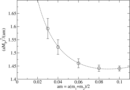
Figure 12: Evidence for quenched chiral logs.

Having already ruled out that the non-zero intercept may be due to the effect of fermion zero modes (the $PP$ and $PP-SS$ correlators produce statistically indistinguishable results for the intercept), the small deviation from linear behavior could be due to finite volume effects or to chiral logs. Insofar as finite volume effects are concerned, not having the resources needed to repeat the calculation on a larger lattice, we can only observe that the Compton wavelength for our lightest pseudoscalar, $M_{P}^{-1}\simeq 4.5a$, is much smaller than the size of our lattice, $L=18a$ ($M_{P}L=4$). In the rest of this section, we compare our results for small quark masses with the predictions from quenched chiral perturbation theory Sharpe (1992); Bernard and Golterman (1992).

We fit the degenerate quark mass results for the pseudoscalar masses to the expression Sharpe (1992)

$$(aM_{P})^{2}=A(am)^{1/(1+\delta)}+B(am)^{2}\;,$$ (19)

where the leading quenched logarithms proportional to $\delta=2m_{0}^{2}/(N_{c}(4\pi f_{\chi})^{2})$ have been resummed into a power behavior and where the term proportional to $B$ parameterizes possible higher-order corrections in the mass expansion. Here $m_{0}$ is the singlet contribution to the $\eta^{\prime}$ mass, $N_{c}=3$ the number of colors, and $f_{\chi}$ the value of the pion decay constant in the chiral limit. The fit is shown in Fig. 12, and the results for the parameters are

$$A=0.680(68),\ \ B=2.98(31),\ \ \delta=0.29(5)\;,$$ (20)

consistent with values of $\delta$ presented elsewhere in the literature Kim and Ohta (2000); Blum et al. (2004); DeGrand and Heller (2002); Aoki et al. (2003); Draper et al. (2003); Gattringer et al. (2004); Chiu et al. (2005). Note that a fit to $(aM_{P})^{2}$ in Eq. (19) containing an additional constant term $C$ does not change the central values of $A$, $B$, or $\delta$ and produces a value for $C$ that is very small and consistent with zero.

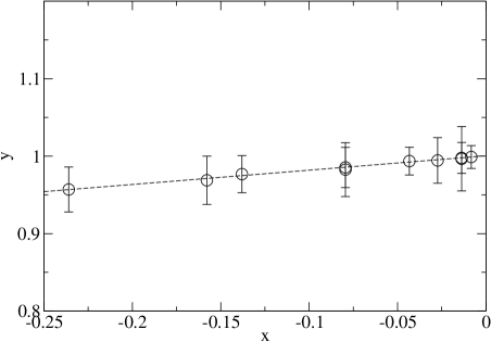
Figure 13: Calculating the quenched chiral log parameter $\delta$ with non-degenerate quark masses.

For the non-degenerate quark case, a value for the quenched chiral log parameter $\delta$ was obtained via a fit to the expression $y=1+\delta\,x$ Bernard and Golterman (1992); Aoki et al. (2003), where

$$y=\,\frac{2m_{1}}{m_{1}+m_{2}}\,\,\frac{M_{12}^{2}}{M_{11}^{2}}\,\,\frac{2m_{2}}{m_{1}+m_{2}}\,\,\frac{M_{12}^{2}}{M_{22}^{2}}\,\;,$$ (21)

$$x=2+\,\frac{m_{1}+m_{2}}{m_{1}-m_{2}}\,\,\ln\left(\,\frac{m_{2}}{m_{1}}\,\right)\;,$$ (22)

and $M_{ij}$ is the mass of a pseudoscalar meson composed of quarks with masses $m_{i}$ and $m_{j}$. In the derivation of this functional form, the contributions of the kinetic term of the singlet Lagrangian with coupling $\alpha$, which is subleading in a $1/N_{c}$ counting, were neglected, as they were in Eq. (19). However, here the quenched chiral log proportional to $\delta$ is considered a correction and dealt with at linear order. In addition, all higher order terms in the chiral expansion are neglected. The value of $\delta$ from our non-degenerate data is

$$\delta=0.18(8)\;,$$ (23)

which is consistent, within the large statistical errors, with the result in Eq. (20).

As shown in Section II.2, these chiral logarithms induce only a small deviation from linear behavior in the relation of $(aM_{P})^{2}$ vs. $(am)$ at the values of light quark mass used in our simulation. Moreover, our statistical errors are still large and our lightest pseudoscalar meson has a mass around that of the kaon, where the quenched theory is tuned to reproduce the unquenched theory. Therefore, we take the slope parameter ${\cal B}$, obtained from the linear fit of Eqs. (9) and (10), to be our estimate of the coefficient of the leading term in the chiral expansion of $(aM_{P})^{2}$ as a function of quark mass $am$.

II.6 Decay constants and determination of the lattice spacing

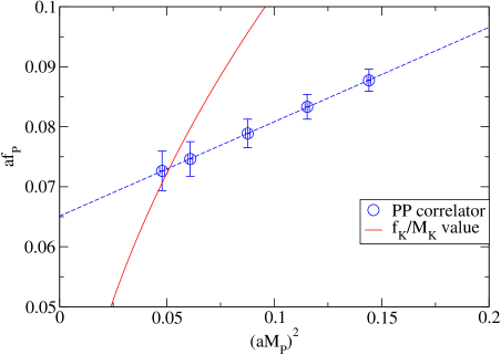
Figure 14: Results for $f_{P}$ and determination of $a$ from the method of physical planes. The dashed line corresponds to a linear fit of the data for $af_{P}$ in the interval $am\leq 0.1$; the solid curve represents the parabola $(af_{P})/(aM_{P})=(f_{K}/M_{K})_{\text{exp}}$.

We extract the decay constant $f_{P}$ from the relation

$$2m|\langle 0|P|\pi\rangle|=2m\sqrt{Z}=f_{P}M_{P}^{2}\;,$$ (24)

where the correlator matrix element $Z$ is defined in Eq. (7). Our results for the pseudoscalar decay constant are reproduced in Fig. 14, where we plot $af_{P}$ as a function of $(aM_{P})^{2}$, together with a line representing the results of a linear fit, as predicted by NLO quenched chiral perturbation theory Sharpe (1992); Bernard and Golterman (1992). Following Allton et al. (1997), we also determine the lattice spacing by the method of lattice physical planes. In particular, we are looking for the point in our lattice parameter space, at which the dimensionless ratio of the pseudoscalar mass and decay constant is equal to the experimentally determined ratio of the Kaon mass to decay constant. The parabola in Fig. 14 shows the line, along which

$$\frac{af_{P}}{aM_{P}}=\Big{(}\frac{f_{K}}{m_{K}}\Big{)}_{\text{exp}}=0.323\;,$$ (25)

where $(f_{K}/M_{K})_{\text{exp}}$ stands for the experimental value of this ratio and we used as experimental data $M_{K}=0.495\,\text{GeV}$ and $f_{K}=0.16\,\text{GeV}$ Eidelman et al. (2004). The intersection of the two lines gives

$$aM_{K}=0.226(6),\qquad af_{K}=0.074(2)\;,$$ (26)

from which, using the input $M_{K}=0.495\,\text{GeV}$, one gets

$$a^{-1}=2.19(6)\,\mathrm{GeV}\;.$$ (27)

Using the Sommer scale value of the lattice spacing and the experimental value of the pion mass, $M_{\pi}=0.135\,\mathrm{GeV}$ Eidelman et al. (2004), yields

$$af_{\pi}=0.065(2)\;,$$ (28)

and thus

$$\,\frac{f_{K}}{f_{\pi}}\,=1.13(4)\;,$$ (29)

which is below the experimental value of 1.22 but is compatible with other quenched calculations Butler et al. (1994); Becirevic et al. (1998); Burkhalter et al. (1999); Heitger et al. (2000); Gattringer et al. (2005).

The method of lattice physical planes has the advantage of using data in a region of quark masses accessible to the lattice calculation, avoiding the need to perform a chiral extrapolation to low quark mass.

The value for $a^{-1}$ derived with the method of lattice physical planes should be contrasted with the one derived from the Sommer scale, namely $a^{-1}=2.12\,\text{GeV}$ at $\beta=6$. A further independent determination of the lattice spacing can be obtained by extrapolating our results for the vector meson spectrum to the chiral limit. This gives $aM_{\rho}=0.409(15)$ (see Eq. (18)), from which one would infer

$$a^{-1}=1.90(4)\,\mathrm{GeV}\;.$$ (30)

The discrepancy among the three values of $a$ obtained above, namely $a^{-1}=1.90(7)\,\text{GeV}$ from the $\rho$ mass, $a^{-1}=2.12\,\text{GeV}$ from the Sommer scale, and $a^{-1}=2.19(6)\,\text{GeV}$ from the method of physical planes, is substantially larger than what could be due to statistical errors alone and should be attributed for the most part to the quenched approximation. The other sources of error, namely those due to the finite lattice spacing, extrapolation to small quark masses, and finite volume effects, are substantially smaller, as can be inferred from the data presented in this paper or, insofar as finite volume effects are concerned, argued from the size of the lattice. Taking the maximum variance in the three numbers above, $\Delta a^{-1}=0.29\,\text{GeV}$, as an indication of the systematic errors in the quenched approximation, the corresponding relative error is $\Delta a^{-1}/a^{-1}\simeq 14\%$. In the rest of this paper, whenever we quote quantities in physical units rather than lattice units, we will use the value of $a^{-1}$ from the Sommer scale for the conversion and systematic errors on such quantities, when given, will include an estimate of the scale setting ambiguity from the method of physical planes.

Equation (26) together with the linear fit of Eqs. (9) and (10), which was justified at the end of Section II.5, gives us

$$a(m_{s}+\hat{m})=0.0661(44)\;,$$ (31)

where $m_{s}$ stands for the bare mass of the $s$-quark and $\hat{m}$ for the average bare mass of the light $u$ and $d$ quarks. We note in passing that using the value of Eq. (31), together with our results for the vector meson masses (from the extended sink correlators), give

$$\,\frac{M_{K^{*}}}{M_{\rho}}\,=1.09(5)\;,$$ (32)

which is compatible within errors with the experimental value of 1.15 as well as with other quenched calculations Becirevic et al. (1998). Use of the Sommer scale value of the lattice spacing, together with our data for the pseudoscalar spectrum and the experimental value for the kaon mass, produces a slightly larger value for $a(m_{s}+\hat{m})$ than the one obtained from the method of physical planes, namely

$$a(m_{s}+\hat{m})=0.0709(17)\;.$$ (33)

We will use this value in the rest of the paper. The variation that the change in $a(m_{s}+\hat{m})$ induces in the values already quoted for $f_{K}/f_{\pi}$ and $M_{K^{*}}/M_{\rho}$ are minimal and well below the statistical errors.

We calculated the vector decay constant using

$$af_{V}=aZ_{V}\sqrt{\,\frac{Z}{M_{V}^{2}}\,}\;,$$ (34)

where $Z$ is the matrix element appearing in the cosh fit of the point source, point sink vector meson correlator and $Z_{V}$ is the renormalization constant of the ultralocal vector current. For $M_{V}$, we used the extended sink vector masses. Like the axial current, the conserved vector current in the overlap discretization is a local, but not ultralocal, operator, and the ultralocal current used in the vector meson correlator must be renormalized. The chiral symmetry properties of the overlap formulation guarantee, however, that $Z_{V}=Z_{A}$, and so we can use the result obtained in Sect. II.3.

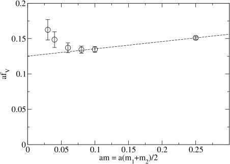
Figure 15: Vector decay constant vs. bare quark mass.

Unfortunately, as described in Sect. II.4, the the coupling of the vector meson ground state to the point sink is rather small. Therefore it is difficult to find a valid plateau range especially for small quark masses. In fact, as can be seen in Fig. 11, only at around $am>0.08$ do the masses extracted from point and extended sink propagators coincide. We therefore also expect the $Z$ extracted from smaller masses to be heavily affected by excited state contributions and choose to ignore them. Consequentlly, we only use the points with quark mass $am=0.08,0.10,0.25$ in the fit of the $af_{V}$ data. Our results for $af_{V}$ are shown in Fig. 15. A linear fit of the data, along with the quark mass of Eq. (33), yields

$$af_{\rho}=0.125(5),\ \ af_{K^{*}}=0.128(5),\ \ \,\frac{f_{K^{*}}}{f_{\rho}}\,=1.03(6)\;.$$ (35)

The ratio $f_{K^{*}}/f_{\rho}$ agrees well with the experimental value 1.03(4) Becirevic et al. (1998).

Using the Sommer scale value for the lattice spacing, the above results give in turn

$$f_{\rho}=265(11)\,\mathrm{MeV},\ \ \ f_{K^{*}}=272(10)\,\mathrm{MeV}\;.$$ (36)

II.7 Quark masses and chiral condensate

Our result for the bare quark masses, $a(m_{s}+\hat{m})$, can be converted into a corresponding result for the renormalized quark masses. The bare quark mass $m(a)$ is related to the renormalized quark mass $\bar{m}(\mu)$ by

$$\bar{m}(\mu)=\lim_{a\to 0}Z_{m}(a\mu)m(a)\;.$$ (37)

The mass renormalization constant $Z_{m}$ is in turn related to the renormalization constant $Z_{S}$ for the non-singlet scalar density by $Z_{m}(a\mu)=1/Z_{S}(a\mu)$. We calculated $Z_{S}$ in the RI-MOM scheme starting from the identity

$$Z_{S}^{\text{RI}}(a\mu)=\lim_{m\to 0}Z_{A}\left.\frac{\Gamma_{A}(p,m)}{\Gamma_{S}(p,m)}\right|_{p^{2}=\mu^{2}}\;,$$ (38)

where $\Gamma_{A}(p,m)$ and $\Gamma_{S}(p,m)$ are suitably defined Green’s functions for the axial current and the scalar density in Landau gauge and $Z_{A}$ is the renormalization constant for the axial current calculated in Sect. II.3. Details of the procedure will be presented in a separate publication. The Green’s functions in Eq. (38) have been calculated non-perturbatively in a window of momenta which extends into the perturbative QCD domain, where contact can be made with perturbatively calculated renormalization constants. We extracted our central value of $Z_{S}$ by performing a combined fit to $am=0.03$ and $am=0.1$ data in a momentum range $p^{2}=3-14\,\text{GeV}^{2}$ using four-loop running Chetyrkin and Retey (2000) and additional $(ap)^{2}$ terms to account for discretization effects as well as $1/p^{2}$ and $1/p^{4}$ terms to account for mass effects and other possible subleading terms in the operator product expansion of the relevant correlation function. We obtain

$$Z_{S}^{\text{RI}}(2\,\text{GeV})=1.25(2)(2)\;,$$ (39)

where the first error is statistical and the second is an estimate of the systematic error obtained by varying the fit range and dropping additional terms when indicated. With this result, one can use the three-loop perturbative calculation of the ratio $Z_{S}^{\overline{\text{MS}}}/Z_{S}^{\text{RI}}$ Chetyrkin and Retey (2000) to calculate

$$Z_{S}^{\overline{\text{MS}}}(2\,\text{GeV})=1.44(2)(3)\;.$$ (40)

Putting together Eqs. (33) and (40), we obtain

$$(m_{s}+\hat{m})^{\overline{\text{MS}}}(2\,\text{GeV})=105(3)(4)\,\mathrm{MeV}$$ (41)

for the sum of strange and light quark masses. Using the value $m_{s}/\hat{m}=24.4(1.5)$ from chiral perturbation theory Leutwyler (1996), we obtain

$$m_{s}^{\overline{\text{MS}}}(2\,\text{GeV})=101(3)(4)\,\mathrm{MeV}$$ (42)

for the strange quark mass, which agrees well with the quenched lattice world average Lubicz (2001); Durr and Hoelbling (2005); Gattringer et al. (2005).

In the unquenched theory, the bare chiral condensate with valence overlap quarks is defined as

$$\chi(a)\equiv\lim_{m\to 0}\,\frac{1}{N_{f}}\,\left\langle\bar{\psi}(0)\left[\left(1-\,\frac{a}{2\rho}\,D\right)\psi\right](0)\right\rangle\;,$$ (43)

where $m$ is the common mass given to the light quarks. It satisfies the integrated non-singlet chiral Ward identity

$$\,\frac{1}{N_{f}}\,\left\langle\bar{\psi}(0)\left[\left(1-\,\frac{a}{2\rho}\,D\right)\psi\right](0)\right\rangle=m\sum_{x}\langle P(x)P^{c}(0)\rangle\;,$$ (44)

where $P$ is the pseudoscalar density composed of two mass-degenerate quarks of different flavor and $P^{c}$ is the density obtained by interchanging the quark flavors. Inserting a complete set of states in $\langle P(x)P^{c}(0)\rangle$ gives

$$\chi(a)=-\lim_{m\to 0}\,\frac{m}{M_{P}^{2}}\,|\langle 0|P|P\rangle|^{2}\;,$$ (45)

where $M_{P}$ is the mass of the pseudoscalar state $|P\rangle$. Using

$$2m|\langle 0|P|\pi\rangle|=f_{P}M_{P}^{2}\;,$$ (46)

where $f_{P}$ is the pseudoscalar decay constant, yields the familiar Gell-Mann-Oakes-Renner (GMOR) relation

$$\chi(a)=-\lim_{m\to 0}\,\frac{f_{P}^{2}M_{P}^{2}}{4m}\,\;.$$ (47)

Due to quenched chiral logarithms, $\chi(a)$ is ill-defined in quenched QCD. However, as argued in Section II.5, the slope parameter $\mathcal{B}$, obtained from the linear fit of Eqs. (9) and (10), should be a reasonable estimate of $\lim_{m\to 0}\,M_{P}^{2}/m$. Thus, we take

$$\chi(a)=-\,\frac{1}{4}\,f_{\chi}^{2}\,\mathcal{B}\,a^{-1}$$ (48)

as our determination of the physical quark condensate. Using our data for $f_{P}$ we get

$$a^{3}\chi(a)=-0.00144(10)$$ (49)

or

$$\chi(a)=-0.0137(10)\,\text{GeV}^{3}\;.$$ (50)

Note that using the value $f_{\chi}=0.123\,\text{GeV}$ Amoros et al. (2001) would instead give $\chi(a)=-0.0110(1)\,\text{GeV}^{3}$.

Using $\langle\bar{\psi}\psi\rangle^{\overline{\text{MS}}}=Z_{S}^{\overline{\text{MS}}}\chi(a)$, we finally get

$$\langle\bar{\psi}\psi\rangle^{\overline{\text{MS}}}(2\,\text{GeV}) = -0.0197(14)(20)\,\text{GeV}^{3}$$ (51)

$$= -[270(6)(9)\,\text{MeV}]^{3}\;.$$

Our results for $m_{s}$ and $\langle\bar{\psi}\psi\rangle$ are in good agreement with the results presented in Giusti et al. (2001). The values were $m_{s}^{\overline{{\text{M}S}}}(2\,\mathrm{GeV})=102(6)(18)\,\mathrm{MeV}$ and $\langle\bar{\psi}\psi\rangle^{\overline{\text{MS}}}(2\,\text{GeV})=-[267(5)(15)\,\text{MeV}]^{3}$. They also agree with the determinations of the condensate using finite-size scaling techniques Hernández et al. (1999a); Hernández et al. (2001), as well as with the recent continuum-limit calculation of Wennekers and Wittig (2005), all of which were obtained using overlap fermions.

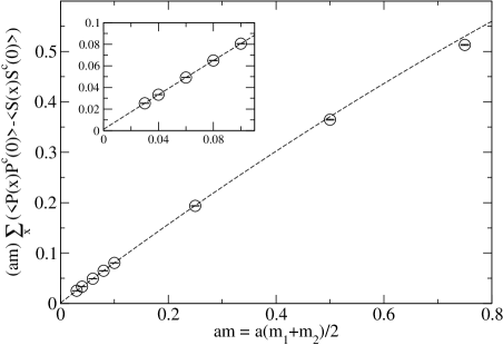
Figure 16: Direct determination of the chiral condensate. The curve corresponds to a quadratic fit of the data according to Eq. (54) in the interval $am\leq 0.1$.

One could also attempt a determination of $\chi$ directly from a fit to the mass dependence of the quantity

$$-a^{3}\hat{\chi}(m) = am\sum_{x}\langle P(x)P^{c}(0)\rangle$$ (52)

$$= \left\langle\bar{\psi}(0)\left[\left(1-\,\frac{a}{2\rho}\,D\right)\psi\right](0)\right\rangle\;.$$

This is, however, made difficult by the very steep dependence of $\hat{\chi}(m)$ on $m$ and also by possible infrared divergent contributions from zero modes. Contrary to the case of the determination of the pseudoscalar spectrum, where we found the effect of zero modes to be suppressed because of the large size of our lattice, zero modes are likely to contribute to the expression in Eq. (52), because it involves the short distance behavior of the quark propagator. The contribution from zero modes can be eliminated by instead considering the subtracted expression

$$-a^{3}\tilde{\chi}(m)=am\sum_{x}(\langle P(x)P^{c}(0)\rangle-\langle S(x)S^{c}(0)\rangle)\;,$$ (53)

which has the same $m\to 0$ limit as $am\sum_{x}(\langle P(x)P^{c}(0)\rangle$ and where the contributions from chiral zero modes cancel. Of course, in the quenched theory, that quantity diverges in the chiral limit due to quenched chiral logarithms. However, here again the effect of the quenched chiral logarithms appear to be small for the light quark masses reached in our simulation, and we assume that a polynomial extrapolation of our quenched results to the chiral limit gives a reliable estimate of the physical condensate. Our results for $-a^{3}\tilde{\chi}(m)$ are shown in Fig. 16. A quadratic fit

$$-a^{3}\tilde{\chi}(m)=-a^{3}\chi+{\cal B}(am)+{\cal C}(am)^{2}$$ (54)

gives the result

$$-a^{3}\chi=0.00131(8)\;,\ \ {\cal B}=0.806(3)\;,\ \ {\cal C}=-0.14(1)\;.$$ (55)

The value we obtain in this way for $a^{3}\chi$ is compatible with the value in Eq. (49). The renormalized value is

$$\langle\bar{\psi}\psi\rangle^{\overline{\text{MS}}}(2\,\text{GeV}) = -0.0179(11)(18)\,\text{GeV}^{3}$$ (56)

$$= -[262(5)(9)\,\text{MeV}]^{3}\;.$$

III Meson Scaling Analysis

Here we present our results for the coarser $14^{3}\times 48$ lattice, with $\beta=5.85$, as well as comparisons between the two lattices.

III.1 Meson spectra

We extract meson masses from the correlators $G_{PP}(t)$ and $G_{PP-SS}(t)$. The effective mass plateau is plotted in Fig. 17 for quark mass $am=0.106$. The data suggest use of a symmetrized fit range $10\leq t/a\leq 24$ in order to extract the pseudoscalar mass.

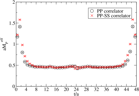
Figure 17: Pseudoscalar effective mass plateau for different channels at $am=0.106$.

The extracted meson masses and matrix elements using this fit range are reported in Tables 6 and 7 in Appendix B. We neglect for the moment chiral logarithms and perform a fit to

$$(aM_{P})^{2}={\cal A}+{\cal B}(am)\;.$$ (57)

Fitting all data with $am\leq 0.132$, we obtain (see Fig. 18)

$${\cal A}=0.0045(15)\;,\qquad{\cal B}=1.923(16)$$ (58)

in the $PP$ channel and

$${\cal A}=0.0007(29)\;,\qquad{\cal B}=1.959(23)$$ (59)

in the $PP-SS$ channel. In general, as for the $18^{3}\times 64$ lattice, the $PP$ and $PP-SS$ channel results were compatible on the $14^{3}\times 48$ lattice, so all further pseudoscalar data, unless otherwise specified, are from the $PP$ channel.

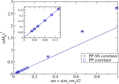
Figure 18: Chiral behavior of meson masses. The lines correspond to the best fit to Eq. (57) in the interval $am\leq 0.132$.

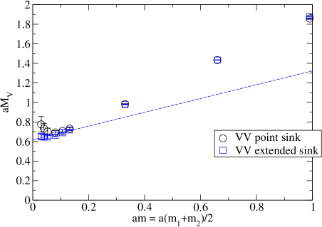
Figure 19: Vector meson masses on the coarser lattice. The line corresponds to the best fit of the extended sink data to Eq. (60) in the interval $am\leq 0.132$.

A fit of the quark-mass dependence of the vector meson mass obtained from the extended sink data, shown in Fig. 19, gives

$$aM_{V}=0.605(29)+0.84(22)\,(am)\;.$$ (60)

We note that the chiral limit value of 0.605(29) is larger than the value 0.483 obtained using the Sommer scale value of the lattice spacing and the experimental $\rho$ mass. As for the finer lattice, we expect that this is a result of quenching errors.

III.2 Axial Ward identity and $Z_{A}$

Figure 20 shows the ratio $\rho(t)=G_{\nabla_{0}A_{0}P}(t)/G_{PP}(t)$ for all of our bare quark masses. We observe a nice plateau for all quark masses, except the largest bare quark mass $am=0.99$, in a range $8\leq t\leq 40$. The lack of a plateau for $am=0.99$ we believe is due to discretization effects, since that quark mass is large and comparable to the inverse lattice spacing.

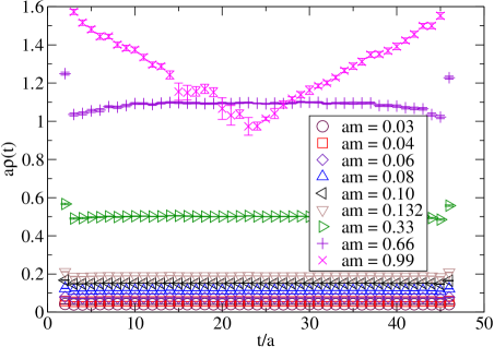
Figure 20: The plateau of the AWI ratio $a\rho(t)$ for different bare quark masses.

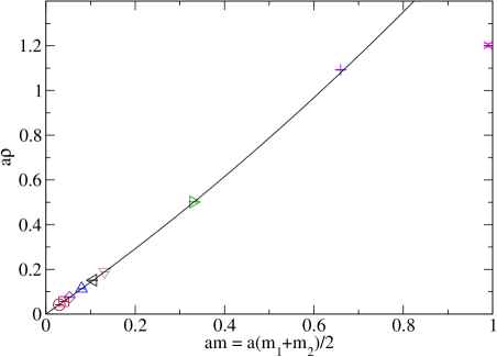
Figure 21: The plateau value of $a\rho$ vs. bare quark mass. The curve corresponds to the best fit to Eq. (14) in the interval $am\leq 0.132$.

Taking the aforementioned plateau range and performing a fit to Eq. (14) with all data for $am\leq 0.132$ (Fig. 21), we obtain

$${\cal A}=0.00004(5)\;,\ \ Z_{A}=1.4434(18)\;,\ \ {\cal C}=0.381(8)\;.$$ (61)

Our results are compatible with chiral symmetry for all bare quark masses except $am=0.99$ and the resulting $Z_{A}$ is in agreement with Bietenholz et al. (2004); Fukaya et al. (2005).

III.3 Quenched chiral logarithms

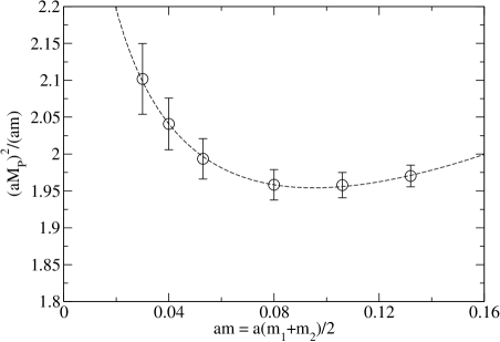
Figure 22: Evidence for quenched chiral logs.

A fit of the degenerate quark mass $PP$ channel results to the expression $(aM_{P})^{2}=A(am)^{1/(1+\delta)}+B(am)^{2}$ of Eq. (19) (see Fig. 22) gives

$$A=1.20(11)\;,\ \ B=2.66(41)\;,\ \ \delta=0.17(4)\;.$$ (62)

Considering the case of unequal quark masses, a fit to the expressions of Eqs. (21) and (22) (see Fig. 23) gives $\delta=0.22(4)$.

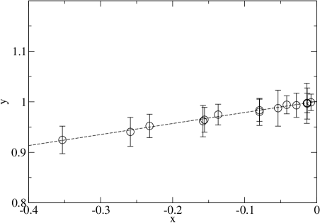
Figure 23: Calculating the quenched chiral log parameter $\delta$.

As discussed in Section II.5 for the results obtained on the finer lattice, we will take the slope parameter $\mathcal{B}$, obtained from the linear fit of Eqs. (57) and (58), to be our estimate of the coefficient of the leading term in the chiral expansion of $(aM_{P})^{2}$ as a function of quark mass $am$.

III.4 Decay constants and determination of the lattice spacing

As for the $18^{3}\times 64$ lattice, we plot in Fig. 24 the lattice decay constant $af_{P}$ versus meson masses $(aM_{P})^{2}$ as obtained by the simulation. The continuous curve represents the physical ratio of these quantities, $(f_{K}/m_{K})_{exp}=0.323$. It turns out that the mesons at our bare quark mass $am=0.053$ correspond most closely to the physical kaons.

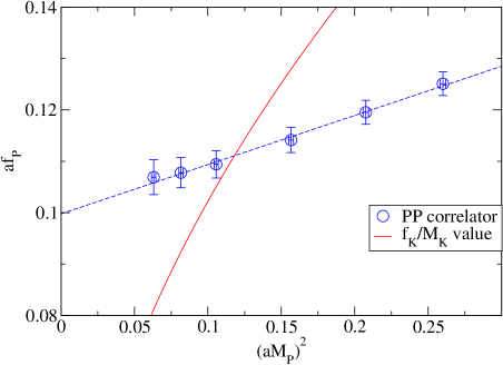
Figure 24: Results for $f_{P}$ and determination of $a$ from the method of physical planes. The dashed line corresponds to a linear fit of the data for $af_{P}$ in the interval $am\leq 0.132$, the solid curve represents the parabola $(af_{P})/(aM_{P})=(f_{K}/M_{K})_{\text{exp}}$.

The intersection of the two curves gives

$$aM_{K}=0.343(9)\;,\qquad af_{K}=0.109(2)\;,$$ (63)

from which, using the input $M_{K}=0.495\,\text{GeV}$, one gets

$$a^{-1}=1.44(4)\,\text{GeV}\;.$$ (64)

Use of the Sommer scale value of the lattice spacing and the experimental pion mass yields

$$af_{\pi}=0.100(3)$$ (65)

and thus

$$\,\frac{f_{K}}{f_{\pi}}\,=1.09(4)\;,$$ (66)

which agrees with Eq. (29).

As for the $18^{3}\times 64$ lattice, the value for $a^{-1}$ derived with the method of lattice physical planes should be contrasted with the one derived from the Sommer scale, namely $a^{-1}=1.61\,\text{GeV}$ at $\beta=5.85$. The lattice spacing obtained by extrapolating our results for the vector meson spectrum to the chiral limit, $aM_{\rho}=0.605(29)$ (see Eq. (60)), is

$$a^{-1}=1.28(6)\,\text{GeV}\;.$$ (67)

As for the finer lattice, the discrepancy between the three values for the lattice spacing can be attributed to the quenched approximation, with a relative error of $\Delta a^{-1}/a^{-1}\simeq 20\%$.

Equation (63), together with the linear fit of Eqs. (57) and (58), which was argued for at the end of Section III.3, gives

$$a(m_{s}+\hat{m})=0.1176(59)\;.$$ (68)

As for the finer lattice, we note in passing that the value of Eq. (68), together with our results for meson masses, give

$$\,\frac{M_{K^{*}}}{M_{\rho}}\,=1.07(6)\;.$$ (69)

Using the Sommer scale value of the lattice spacing and our pseudoscalar spectrum data yields a slightly smaller value for $a(m_{s}+\hat{m})$ of

$$a(m_{s}+\hat{m})=0.0943(15)\;.$$ (70)

We will use this value for the rest of the scaling analysis.

We again calculated the vector decay constant using $af_{V}=aZ_{V}\sqrt{Z/M_{V}^{2}}$. In the fit of the $af_{V}$ data, we used only the points with quark mass $am=0.106,0.132,0.33$, since the point-point correlators give poor results for $Z$ for lower quark masses. Our results for $af_{V}$ are shown in Fig. 25. A linear fit of the data, along with the quark mass of Eq. (70), yields

$$af_{\rho}=0.175(13)\;,\ \ af_{K^{*}}=0.179(12)\;,\ \ \,\frac{f_{K^{*}}}{f_{\rho}}\,=1.02(10)\;.$$ (71)

The ratio $f_{K^{*}}/f_{\rho}$ agrees well with both the value on the finer lattice, Eq. (35), and the experimental value 1.03(4) Becirevic et al. (1998).

Using the Sommer scale value for the lattice spacing, the above results give in turn

$$f_{\rho}=281(22)\,\mathrm{MeV}\;,\ \ \ f_{K^{*}}=287(19)\,\mathrm{MeV}\;.$$ (72)

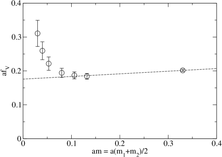
Figure 25: Vector decay constant vs. bare quark mass.

III.5 Quark masses and chiral condensate

As in Section II.7, we calculate $Z_{S}$ in the RI-MOM scheme from

$$Z_{S}^{\text{RI}}(a\mu)=\lim_{m\to 0}Z_{A}\left.\frac{\Gamma_{A}(p,m)}{\Gamma_{S}(p,m)}\right|_{p^{2}=\mu^{2}}\;.$$ (73)

Only data with $am\leq 0.132$ were used for this purpose. In order to obtain our final result, we used a combined fit to $am=0.04$ and $am=0.132$ in the range $p^{2}=2-8\,\text{GeV}^{2}$ for central values and obtained an estimate of the systematic error by varying the fit range and dropping additional terms when indicated. We fit $Z_{S}$ to the same functional form as for $\beta=6.0$, yielding

$$Z_{S}^{\text{RI}}(2\,\text{GeV})=1.29(3)(14)$$ (74)

and

$$Z_{S}^{\overline{\text{MS}}}(2\,\text{GeV})=1.48(3)(16)\;.$$ (75)

Putting together Eqs. (70) and (75), we obtain

$$(m_{s}+\hat{m})^{\overline{\text{MS}}}(2\,\text{GeV})=102(3)(16)\,\text{MeV}$$ (76)

for the sum of the strange and light quark masses. As for the finer lattice, using the value $m_{s}/\hat{m}=24.4(1.5)$ from chiral perturbation theory Leutwyler (1996), we obtain

$$m_{s}^{\overline{\text{MS}}}(2\,\text{GeV})=98(3)(15)\,\mathrm{MeV}$$ (77)

for the strange quark mass, which agrees well with the quenched lattice world average Lubicz (2001); Durr and Hoelbling (2005); Gattringer et al. (2005).

Using the GMOR inspired relation of Eq. (48) and our data for $f_{P}$ we get

$$a^{3}\chi(a)=-0.00473(28)$$ (78)

or

$$\chi(a)=-0.0195(12)\,\text{GeV}^{3}\;.$$ (79)

Note that using the value $f_{\chi}=0.123\,\text{GeV}$ Amoros et al. (2001) would instead give $\chi(a)=-0.0117(1)\,\text{GeV}^{3}$.

Using $\langle\bar{\psi}\psi\rangle^{\overline{\text{MS}}}=Z_{S}^{\overline{\text{MS}}}\chi(a)$, we finally get

$$\langle\bar{\psi}\psi\rangle^{\overline{\text{MS}}}(2\,\text{GeV}) = -0.0292(18)(98)\,\text{GeV}^{3}$$ (80)

$$= -[308(6)(34)\,\text{MeV}]^{3}\;.$$

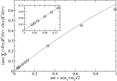
Figure 26: Direct determination of the chiral condensate. The curve corresponds to a quadratic fit of the data according to Eq. (82) in the interval $am\leq 0.132$.

Our results for the direct calculation of $-a^{3}\tilde{\chi}(m)$ using

$$-a^{3}\tilde{\chi}(m)=am\sum_{x}(\langle P(x)P^{c}(0)\rangle-\langle S(x)S^{c}(0)\rangle)$$ (81)

are shown in Fig. 26. The quadratic fit discussed in Section II.7,

$$-a^{3}\tilde{\chi}(m)=-a^{3}\chi+{\cal B}(am)+{\cal C}(am)^{2}\;,$$ (82)

gives the result

$$-a^{3}\chi=0.00448(22)\;,\ \ {\cal B}=0.798(4)\;,\ \ {\cal C}=-0.14(2)\;.$$ (83)

The value we obtain in this way for $a^{3}\chi$ is compatible with the value in Eq. (78). The renormalized value is

$$\langle\bar{\psi}\psi\rangle^{\overline{\text{MS}}}(2\,\text{GeV}) = -0.0277(15)(93)\,\text{GeV}^{3}$$ (84)

$$= -[302(5)(34)\,\text{MeV}]^{3}\;.$$

III.6 Direct comparison of the two lattices

We compare in Figs. 27-29 our results for the pseudoscalar and vector spectra for the finer and coarser lattices, using the Sommer scale value for the lattice spacing to express masses in physical units. We neglect logarithmic effects in the lattice spacing and plot the mass spectra as a function of bare quark mass. It is interesting to observe that our results for the mass spectra on the two different lattices are very similar. A qualitatively equivalent conclusion would be reached with the renormalized quark mass. Our results suggest that the scaling violations for the quantities that we consider may be quite small. However, one has to keep in mind, that we only have data for two values of the lattice spacing and that the mass parameter $\rho$ is not held fixed (for a detailed discussion of this point see Appendix A).

Table 1 in Appendix B shows a direct comparison of data from the two lattices.

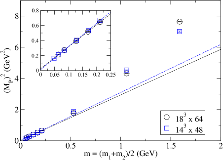
Figure 27: Pseudoscalar $PP$ spectrum comparison.

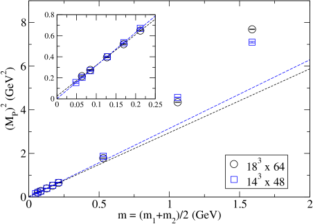
Figure 28: Pseudoscalar $PP-SS$ spectrum comparison.

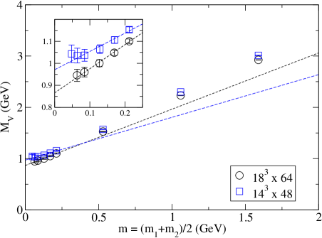
Figure 29: Vector (extended sink) spectrum comparison.

IV Light Baryon Spectra

IV.1 Baryon spectra

The increased temporal extent of our lattice with respect to that in Giusti et al. (2001) has made possible the calculation of the light baryon spectrum. Despite the challenges of limited statistics and the use of point sources and sinks, the lightest octet and decuplet masses were measured, together with those of the corresponding negative-parity states. For other recent determinations of the baryon spectrum with chiral fermions, see Mathur et al. (2005); Dong et al. (2002); Lee et al. (2003); Galletly et al. (2004); Chiu and Hsieh (2005); Aoki et al. (2004); Sasaki (2001); Sasaki et al. (2002).

Baryon correlation functions were constructed with the following interpolating operators. For the octet, we use

$$O^{f_{1}f_{2}f_{3}}_{\alpha}=\epsilon_{abc}(\psi^{f_{1}T}_{a}C\gamma_{5}\psi^{f_{2}}_{b})\psi^{f_{3}}_{c,\alpha}\;,$$ (85)

where $C=\gamma_{2}\gamma_{4}$ is the charge conjugation matrix, $\alpha$ is a Dirac index, $f_{i}$ denotes flavor, and $a,b,c$ denote color. For the decuplet states, we use a notation similar to that in Aoki et al. (2003) and define

$$\Gamma_{\pm}=(\gamma_{2}\mp i\gamma_{1})/2\;,\qquad\Gamma_{0}=i\gamma_{3}\;.$$ (86)

We work in a representation of the Dirac matrices where $\gamma_{4}=\mathrm{diag}(1,1,-1,-1)$. Labeling the channels by $J_{z}$, the decuplet operators are then given by

$$D_{3/2}^{f_{1}f_{2}f_{3}} = \epsilon_{abc}(\psi^{f_{1}T}_{a}C\,\Gamma_{+}\psi^{f_{2}}_{b})\psi^{f_{3}}_{c,\alpha=1}\;,$$ (87)

$$D_{-3/2}^{f_{1}f_{2}f_{3}} = \epsilon_{abc}(\psi^{f_{1}T}_{a}C\,\Gamma_{-}\psi^{f_{2}}_{b})\psi^{f_{3}}_{c,2}\;,$$ (88)

$$D_{1/2}^{f_{1}f_{2}f_{3}} = \epsilon_{abc}[(\psi^{f_{1}T}_{a}C\,\Gamma_{0}\psi^{f_{2}}_{b})\psi^{f_{3}}_{c,1}$$ (89)

$$\qquad+(\psi^{f_{1}T}_{a}C\,\Gamma_{+}\psi^{f_{2}}_{b})\psi^{f_{3}}_{c,2}]/3\;,$$

$$D_{-1/2}^{f_{1}f_{2}f_{3}} = \epsilon_{abc}[(\psi^{f_{1}T}_{a}C\,\Gamma_{0}\psi^{f_{2}}_{b})\psi^{f_{3}}_{c,2}$$ (90)

$$\qquad+(\psi^{f_{1}\,T}_{a}C\,\Gamma_{-}\psi^{f_{2}}_{b})\psi^{f_{3}}_{c,1}]/3\;.$$

Without loss of generality, we may assume that the three quark flavors are distinct and for simplicity call the flavors $u,d,s$. For the results that follow, two quarks are always taken to have the same mass, and assigning them identical flavor would merely change the normalization of the correlator. The two possible octet states may be identified with the $\Sigma^{0}$ and $\Lambda^{0}$ and are given by

$$\Sigma_{\alpha} = O_{\alpha}^{dsu}+O_{\alpha}^{usd}\;,$$ (91)

$$\Lambda_{\alpha} = O_{\alpha}^{dsu}-O_{\alpha}^{usd}-2O_{\alpha}^{uds}\;.$$ (92)

These give identical correlators only when all three quark masses are degenerate. When propagating forward, the $\alpha=1,2$ components of these operators have positive-parity, while the $\alpha=3,4$ components have negative-parity. To extract a mass, we must project out states of definite parity by defining

$$G_{\pm}(t)=\sum_{\mathbf{x}}\langle 0|\Sigma_{\alpha}(\mathbf{x},t)\big{(}\frac{1\pm\gamma_{4}}{2}\big{)}_{\alpha\beta}\bar{\Sigma}_{\beta}(\mathbf{0},0)|0\rangle\;.$$ (93)

The mass $m_{+}$ of the positive-parity state is then extracted by fitting $Ae^{-m_{+}t}=G_{+}(t)+G_{-}(T-t)$ for an appropriate range of times $t$ (where we can neglect the backward-propagating negative-parity contribution to $G_{+}(t)$ and vice versa). Here $T$ is the total extent of the lattice in the time direction. Similarly, $Ae^{-m_{-}t}=G_{-}(t)+G_{+}(T-t)$ yields the mass of the negative-parity state.

For the decuplet we use

$$(\Sigma^{*})_{J_{z}}=D_{J_{z}}^{uds}+D_{J_{z}}^{sud}+D_{J_{z}}^{dsu}$$ (94)

and combine correlators for the four spin states with the corresponding time-reversed correlators of opposite parity. The negative-parity operators are defined by replacing the Dirac index of $\psi^{f_{3}}$ in $D_{J_{z}}^{f_{1}f_{2}f_{3}}$ according to $1\rightarrow 3$, $2\rightarrow 4$.

Here we have followed convention by defining our operators in covariant form. We note, however, that one may also work directly with components and construct the spin wave functions explicitly. For example, using the notation $|\alpha\beta\gamma\rangle=\epsilon_{abc}\psi^{u}_{a,\alpha}\psi^{d}_{b,\beta}\psi^{s}_{c,\gamma}$, alternate operators for the two spin-up octet states are

$$\Lambda = (|121\rangle-|211\rangle)/\sqrt{2}\;,$$ (95)

$$\Sigma = (|121\rangle+|211\rangle-2|112\rangle)/\sqrt{6}\;.$$ (96)

By construction, these have only terms with upper components, whereas the operators given in covariant form also include terms involving lower components (e.g. $|341\rangle$). Contributions from these additional terms are suppressed since the lower components vanish in the non-relativistic limit, and the two types of operators were in fact found to give compatible results for both the octet and decuplet. For the results presented here, only the covariant forms were used.

Baryon masses were calculated at $\beta=6$ with two degenerate quarks having each of the five lightest available masses ($am_{1}=am_{2}=0.03,0.04,0.06,0.08,0.1$) and for all available masses of the third quark (including 0.25, 0.5, and 0.75). Errors were estimated by a bootstrap procedure where correlators for the four or eight spin channels are grouped by configuration prior to sampling. Fitting windows were chosen based on plots of the effective mass $M_{eff}=\mathrm{ln}[C(t-a)/C(t)]$ for $am_{1}=am_{2}=am_{3}=0.03$. The preferred window (used below for chiral fits) was determined by choosing $t_{min}$ such that $M_{eff}(t_{min})$ and $M_{eff}(t_{min}+a)$ are compatible to within $1\,\sigma$ and $t_{max}$ such that the error in $M_{eff}(t_{max})$ (determined by the bootstrap method) does not exceed 30 percent. The latter criterion was made more stringent for the positive-parity decuplet state for reasons described below. The windows chosen on the basis of the lightest quark mass were then used for all other quark masses.

For the octet states, the windows were $8\leq t/a\leq 16$ for $J^{P}=\frac{1}{2}^{+}$ and $6\leq t/a\leq 8$ for $J^{P}=\frac{1}{2}^{-}$. Data for a range of windows are provided in Table 10 in Appendix B. In Fig. 30, we plot the $\Lambda$-like octet masses as a function of total quark mass. Measurements for two values of $t_{min}$ are shown in order to give some indication of the dependence on fitting window. Figure 31 shows the splitting between the two octet states as the mass of the third quark is increased away from $am_{1}=am_{2}=0.03$.

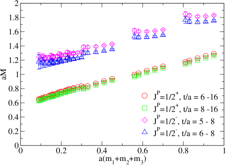
Figure 30: Positive- and negative-parity octet masses for two fitting windows and quark masses $m_{1}=m_{2}$ degenerate.

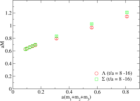
Figure 31: Masses of the two octet states with quark masses $am_{1}=am_{2}=0.03$

Results for the decuplet states are shown in Fig. 32. The data are reproduced for a range of fitting windows in Table 11. We note that the masses of the heavier states ($J^{P}=\frac{1}{2}^{-},\frac{3}{2}^{\pm}$) exhibit a substantial dependence on the fitting window. In particular, the effective mass of the positive-parity decuplet state is seen to first plateau and then, at large times, continue downward toward the octet mass. This behavior may be explained by considering what gives rise to the more rapid fall-off of correlators for excited states. Correlators for the octet and the decuplet are constructed from the same ingredients, the same quark propagators. The more rapid fall-off of the decuplet arises because of cancellations between terms. A fit of the correlator gives a reliable determination of the mass only insofar as these cancellations are not overwhelmed by fluctuations. At large times, the remaining fall-off is due primarily to the constituent masses of the quarks rather than the baryon mass itself. For this reason, we have constrained $t_{max}$ to the value used for the octet, giving the fitting window $8\leq t/a\leq 16$. The uncertainty associated with this choice of window is relatively large and of the same order as the statistical error. The window for the $J^{P}=\frac{3}{2}^{-}$ state is $8\leq t/a\leq 10$. We also note that the windows for both negative-parity states are rather small due to the early onset of fluctuations. For all of these reasons, our results for the negative-parity octet and decuplet states should be considered to have indicative value only.

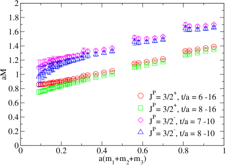
Figure 32: Positive- and negative-parity decuplet masses for two fitting windows and quark masses $m_{1}=m_{2}$ degenerate.

Finally, in Fig. 33 we plot the masses of the positive-parity states for light degenerate quark masses $am_{1}=am_{2}=am_{3}=0.03,0.04,0.06,0.08,0.1$. A linear extrapolation to the chiral limit gives $aM_{8}=0.559(24)$ and $aM_{10}=0.690(32)$. In this limit, using the value of $aM_{\rho}$ from Eq. (18), we find

$$M_{8}/M_{\rho} = 1.37(8)\;,$$ (97)

$$M_{10}/M_{8} = 1.23(8)\;.$$ (98)

The limited statistics of our data do not warrant a more complicated fitting form. Experimentally, $M_{N}/M_{\rho}=1.21$ and $M_{\Delta}/M_{N}=1.31$ Eidelman et al. (2004).

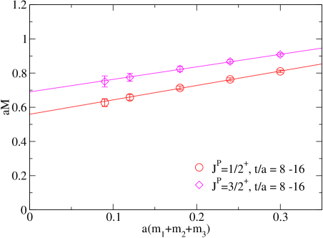
Figure 33: Baryon masses with three light degenerate quarks were extrapolated to the chiral limit with assumed linear dependence on quark mass.

IV.2 Baryon scaling

To investigate scaling, masses of the positive-parity states were also calculated at $\beta=5.85$ on the $14^{3}\times 48$ lattice. In light of the small fitting windows that had been required on the finer lattice, fits for the corresponding negative-parity masses were not attempted. Here we find $aM_{8}=0.741(28)$ and $aM_{10}=1.033(55)$ in the chiral limit, yielding

$$M_{8}/M_{\rho} = 1.23(8)\;,$$ (99)

$$M_{10}/M_{8} = 1.39(9)\;.$$ (100)

As in the meson analysis, we make use of the Sommer scale, which gives $a^{-1}=2.12$ GeV at $\beta=6$ and $a^{-1}=1.61$ GeV at $\beta=5.85$. Figure 34 shows the $J^{P}=\frac{1}{2}^{+}$ and $J^{P}=\frac{3}{2}^{+}$ states for light degenerate quarks on both lattices. Bare masses are rescaled by the corresponding values of $a^{-1}$. We see that the octet spectrum exhibits good scaling while the decuplet shows some indication of scaling violation. Comments in Section III.6 regarding renormalized quark masses, however, apply here as well. Also, as we have already observed, the decuplet masses suffer from uncertainty in the choice of fitting window and so the apparent lack of scaling should not be considered to have much significance.

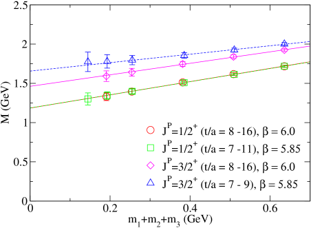
Figure 34: Baryon masses with light degenerate quarks at two values of $\beta$, with lattice spacing set by the Sommer scale.

V Diquark Correlations

V.1 Diquark correlators

In the past two years, experiments have produced indications of bound quark systems beyond the usual quark-antiquark mesons and three quark baryons Nakano et al. (2003); Barmin et al. (2003); Stepanyan et al. (2003); Barth et al. (2003); Hicks (2005). The most prominent example is the five particle $\Theta^{+}(1540)$ pentaquark. The reality of such states is in question, since a number of attempts at verifying the pentaquark observations have failed Bai et al. (2004); Aubert et al. (2004); Abe et al. (2004); Armstrong (2005); Abt et al. (2004); Antipov et al. (2004); Longo et al. (2004); Litvintsev (2005).

Nevertheless, lattice calculations should provide a definitive check on whether QCD predicts such states. In certain models Jaffe and Wilczek (2003) of the $\Theta^{+}(1540)$, which consists of the bound valence quarks $uudd\bar{s}$, the four quarks bind into two pairs of diquarks, and the two diquarks bind with the remaining $\bar{s}$.

Information on possible diquark states can be obtained by measuring diquark correlations on the lattice Csikor et al. (2003). A study of correlations inside baryons, using a method similar to the one we used to investigate the $q\bar{q}$ wave functions in Section II.4, is in progress.

The fact that our propagators were calculated in Landau gauge allows us also to measure quark-quark correlations directly and to fit their decay in Euclidean time in terms of an effective “diquark mass” Hess et al. (1998). Of course, because of the gauge fixing, one should not consider such a mass parameter to be the mass of a physical state. Nevertheless, it can produce an indication of the relative strength of quark bindings inside diquark states. We consider correlations for the diquark operators

$$\mathcal{O}_{c}^{s_{1}s_{2}}(x)=\epsilon_{cc_{1}c_{2}}\psi_{c_{1}}^{s_{1}}(x)\,\psi_{c_{2}}^{s_{2}}(x)\;,$$ (101)

and

$$\mathcal{O}_{c_{1}c_{2}}^{s_{1}s_{2}}(x)=\,\frac{1}{\sqrt{2}}\,(\psi_{c_{1}}^{s_{1}}(x)\,\psi_{c_{2}}^{s_{2}}(x)+\psi_{c_{2}}^{s_{1}}(x)\,\psi_{c_{1}}^{s_{2}}(x))\;,$$ (102)

which are a ${\bf\bar{3}}$ and ${\bf 6}$ of color, respectively. Using these operators, we form four types of diquark states: (i) color ${\bf\bar{3}}$, spin-0, flavor ${\bf\bar{3}}$, (ii) color ${\bf\bar{3}}$, spin-1, flavor ${\bf 6}$, (iii) color ${\bf 6}$, spin-0, flavor ${\bf 6}$, and (iv) color ${\bf 6}$, spin-1, flavor ${\bf\bar{3}}$.

Diquark correlation functions for $am_{1}=0.03$ and $am_{2}=0.03$, the lightest quark mass combination, are displayed in Figs. 35-38. Since $\gamma_{4}$ was diagonal in the $\gamma$-matrix basis we used, upper components were combined with time-reversed lower components to form positive-parity states, while mixed upper and lower components were combined to form negative-parity states. Figure 39 shows a plot of the quark correlator for input quark mass 0.03.

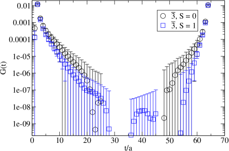
Figure 35: ${\bf\bar{3}}$ positive-parity diquark correlation function; $am_{1}=0.03$, $am_{2}=0.03$.

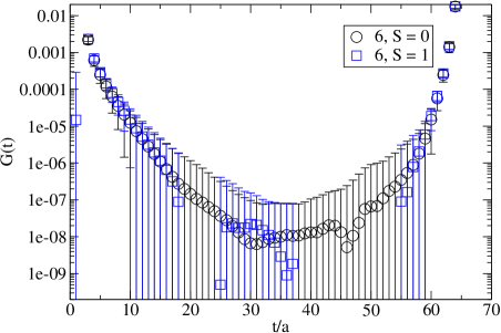
Figure 36: ${\bf 6}$ positive-parity diquark correlation function; $am_{1}=0.03$, $am_{2}=0.03$.

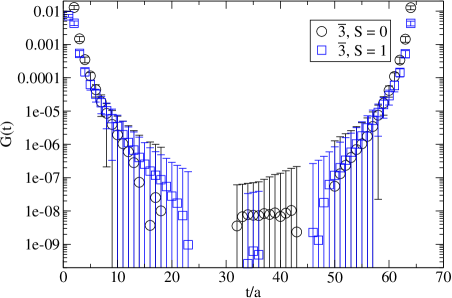
Figure 37: ${\bf\bar{3}}$ negative-parity diquark correlation function; $am_{1}=0.03$, $am_{2}=0.03$.

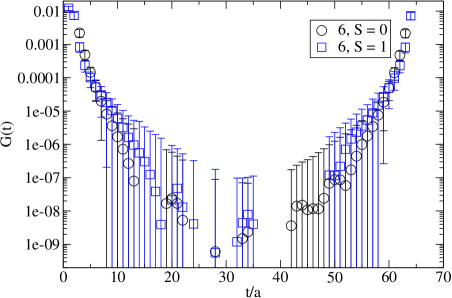
Figure 38: ${\bf 6}$ negative-parity diquark correlation function; $am_{1}=0.03$, $am_{2}=0.03$.

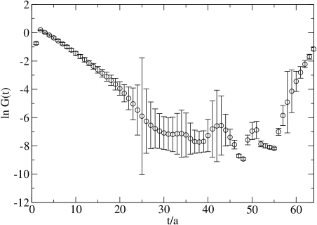
Figure 39: Quark correlation function for input mass $am=0.03$.

V.2 Diquark spectra

Figure 40 shows the (positive-parity) diquark spectrum and the constituent quark masses as a function of input quark mass. The fitting window used was $5\leq t/a\leq 15$. That figure also includes a plot of twice the constituent quark mass and extrapolations to zero quark mass for the “twice quark mass” and ${\bf\bar{3}}$ spin-0 results. Figure 41 shows the same for the negative-parity states, with a fit for the lowest energy diquark state, the ${\bf\bar{3}}$ spin-1.

It is interesting to observe that the ${\bf\bar{3}}$ diquark spin-0 extrapolation in Fig. 40 is below twice the quark mass extrapolation and that the ${\bf\bar{3}}$ diquark spin-0 state is significantly more strongly bound than the ${\bf\bar{3}}$ diquark spin-1 state. Such a result is consistent with the predictions of diquark models Anselmino et al. (1993); Jaffe and Wilczek (2003). However, a much more detailed analysis must be done, particularly on diquarks within baryon states, in order for rigorous conclusions to be reached.

The diquark data is shown in Tables 14 and 15 in Appendix B. Constituent quark masses, calculated from fits ($5\leq t/a\leq 15$) to the quark correlators, are shown in Table 16 in Appendix B.

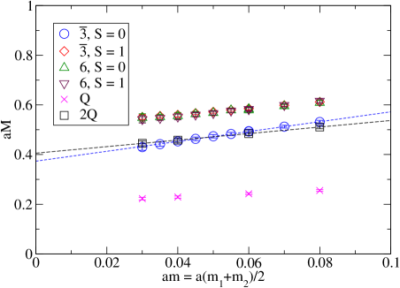
Figure 40: Diquark spectrum vs. input quark mass, positive-parity.

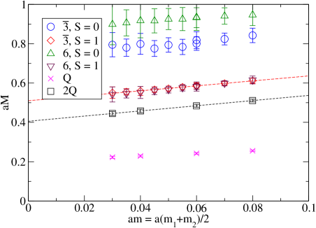
Figure 41: Diquark spectrum vs. input quark mass, negative-parity.

VI Conclusions

In this article, we have presented results from quenched lattice QCD simulations using the overlap Dirac operator on an $18^{3}\times 64$ lattice at $\beta=6.0$ and a $14^{3}\times 48$ lattice at $\beta=5.85$. We calculated quark propagators with a fixed source point and a variety of quark mass values for 100 configurations on each lattice, and we have used them to evaluate meson and baryon observables, quark masses, meson final-state wave functions, and diquark correlations.

One important result of our work is that the calculation of quark propagators with the overlap operator to a chosen numerical precision has been shown to be feasible using available techniques, even when dealing with rough background gauge configurations. Such a calculation requires projection of low lying eigenvectors of $H^{2}=(\gamma_{5}D_{W})^{2}$. Improved algorithms or smoothing techniques both may help to make the calculation less computationally demanding Durr et al. (2005).

Beyond this, our investigation validates the good chiral properties of the overlap operator and suggests good scaling properties between $\beta=5.85$ and $\beta=6$, indicating that the $\beta=6$ results may already be close to the continuum limit. So far as the actual values of the observables are concerned, our results suffer from the shortcomings of the quenched approximation. Nevertheless, from this investigation and others it is clear that it should be possible to use the overlap operator in dynamical fermion simulations, at the very least with a mixed action formulation. Work in that direction is beginning. We are also working to extend our diquark results to diquark correlations in baryons with one heavy and two light quarks, and we expect to soon publish our results on non-perturbative renormalization, selected weak matrix elements, and heavy quark observables.

Appendix A The Overlap Formalism and Simulation Details

The forward and backward lattice covariant derivatives are defined by

$$\nabla_{\mu}\psi(x)=\,\frac{1}{a}\,[U_{\mu}(x)\psi(x+a\hat{\mu})-\psi(x)]\;,$$ (103)

and

$$\nabla_{\mu}^{*}\psi(x)=\,\frac{1}{a}\,[\psi(x)-U_{\mu}^{\dagger}(x-a\hat{\mu})\psi(x-a\hat{\mu})]\;,$$ (104)

where $U_{\mu}(x)$ are the gauge link fields on the lattice. Let $D_{W}$ denote the Wilson-Dirac operator

$$D_{W}=\,\frac{1}{2}\,\gamma_{\mu}(\nabla_{\mu}+\nabla_{\mu}^{*})-\,\frac{r}{2}\,a\,\nabla_{\mu}^{*}\nabla_{\mu}\;,$$ (105)

with $0<r\leq 1$ and $0<\rho<2r$ (we used $r=1$ in our calculations) and where $a$ is the lattice spacing.

Neuberger’s overlap Dirac operator is then defined as Narayanan and Neuberger (1995b); Neuberger (1998b)

$$D=\,\frac{\rho}{a}\,(1+V)=\,\frac{\rho}{a}\,\left(1+\gamma_{5}H\,\frac{1}{\sqrt{H^{\dagger}H}}\,\right)\;,$$ (106)

where

$$H=\gamma_{5}(D_{W}-\,\frac{1}{a}\,\rho)$$ (107)

and $\rho$ is a parameter that affects the radius of rescaling of eigenvalues of the overlap operator in the complex plane as compared to the Wilson-Dirac operator.

The combination of the Wilson gauge action and the (massive) overlap fermionic action is

$$S = \,\frac{6}{g_{0}^{2}}\,\sum_{P}\left[1-\,\frac{1}{6}\,\mathrm{Tr}\,(U_{P}+U_{P}^{\dagger})\right]$$ (108)

$$\qquad+\bar{\psi}\left[\left(1-\,\frac{a}{2\rho}\,\,m\right)D+m\right]\psi\;,$$

where $U_{P}$ is the Wilson plaquette, $g_{0}=\sqrt{6/\beta}$ is the bare coupling constant, the fermion fields $\psi$ and $\bar{\psi}$ carry implicit color, spin, and flavor indices, and $m$ is a diagonal matrix of bare masses $(m_{1},m_{2},\dots)$ in flavor space.

The Ginsparg-Wilson relation Ginsparg and Wilson (1982b)

$$\gamma_{5}D+D\gamma_{5}=\,\frac{a}{\rho}\,D\gamma_{5}D$$ (109)

is satisfied by the fermionic operator of the overlap action, implying an exact continuous symmetry of the action in the massless limit Lüscher (1998). The symmetry can be interpreted as a lattice form of chiral invariance at finite cutoff,

$$\delta\psi=\hat{\gamma}_{5}\psi,\ \ \ \delta\bar{\psi}=\bar{\psi}\gamma_{5}\;,$$ (110)

where

$$\hat{\gamma}_{5}\equiv\gamma_{5}\left(1-\,\frac{a}{\rho}\,D\right)\;,$$ (111)

which satisfies $\hat{\gamma}_{5}^{\dagger}=\hat{\gamma}_{5}$ and $\hat{\gamma}_{5}^{2}=1$. Invariance of the action under non-singlet chiral transformations, defined including a flavor group generator in Eq. (110), forbids mixing among operators of different chirality Hasenfratz (1998). Therefore,

• no additive quark mass renormalization is required, and the quark mass which enters the vector and axial Ward identities is the bare parameter $m(a)$;

• masses and matrix elements are affected only by $\mathcal{O}(a^{2})$ errors and no fine-tuned parameters are required to remove $\mathcal{O}(a)$ effects;

• and the chiral condensate (see Section II.7) does not require subtractions of power divergent terms (in the chiral limit).

The non-singlet “local” (source and sink at the same point $x$) bilinear operators we use are defined by

$$O_{\Gamma}(x)=\bar{\psi}_{1}(x)\Gamma\left[(1-\,\frac{a}{2\rho}\,D)\psi_{2}\right](x)\;,$$ (112)

where $O_{\Gamma}\in\{S,P,V_{\mu},A_{\mu}\}$ correspond to $\Gamma\in\{\hbox{1$\!\!$1},\gamma_{5},\gamma_{\mu},\gamma_{\mu}\gamma_{5}\}$. (We also use non-local “extended” operators; see Section II.4.) The bilinear operators are subject to multiplicative renormalization only, i.e. the corresponding renormalized operators are

$$\hat{O}_{\Gamma}(x,\mu)=\lim_{a\to 0}Z_{\Gamma}(a\mu)\,O_{\Gamma}(x,a)\;,$$ (113)

where $Z_{\Gamma}(a\mu)$ are the appropriate renormalization constants. Since $S,P$ and $V_{\mu},A_{\mu}$ belong to the same chiral multiplets, $Z_{S}=Z_{P}$ and $Z_{V}=Z_{A}$. Also, flavor symmetry imposes $Z_{S}=1/Z_{m}$, with $Z_{m}$ defined in Eq. (37).

Using such operators, the following two-point correlation functions (or “correlators”) can be formed:

$$G_{SS}(t)=\sum_{\vec{x}}\langle S(\vec{x},t)S^{c}(\vec{0},0)\rangle\;,$$ (114)

$$G_{PP}(t)=\sum_{\vec{x}}\langle P(\vec{x},t)P^{c}(\vec{0},0)\rangle\;,$$ (115)

$$G_{\nabla_{0}A_{0}P}(t)=\sum_{\vec{x}}\langle\bar{\nabla}_{0}A_{0}(\vec{x},t)P^{c}(\vec{0},0)\rangle\;,$$ (116)

$$G_{VV}(t)=\sum_{\vec{x},i}\langle V_{i}(\vec{x},t)V_{i}^{c}(\vec{0},0)\rangle\;,$$ (117)

where we assume the quarks to be of different flavor, $c$ denotes flavor conjugation, i.e. interchange of the two flavors, and $\bar{\nabla}_{0}$ is the symmetric lattice derivative in the time direction. When appropriate, such correlators are symmetrized around $t=T/2$, where $T$ is the extent of the lattice in the time direction.

Our simulations studied quenched QCD with the Wilson gauge action and with Neuberger’s overlap Dirac operator for lattice fermions on two different lattices. For both simulations, we used samples of 100 gauge configurations generated by a 6-hit Metropolis algorithm with acceptance $\simeq 0.5$. The configurations were separated by 10,000 upgrades, after an initial set of 11,000 upgrades for equilibration.

The first simulation was done on an $18^{3}\times 64$ lattice, with $\beta=6$, $\rho=1.4$, and lattice spacing $a^{-1}\simeq 2.0\,\mathrm{GeV}$. We calculated overlap quark propagators for a single point source, for all 12 color-spin combinations and quark masses $am=0.03,0.04,0.06,0.08,0.1,0.25,0.5$ and $0.75$, using a multi-mass solver.

The second simulation was done on a $14^{3}\times 48$ lattice, with $\beta=5.85$ and $\rho=1.6$. The second, coarser lattice was chosen to have roughly the same volume as the finer $18^{3}\times 64$ lattice, with lattice spacing $a^{-1}\simeq 1.5\,\mathrm{GeV}$, allowing for an investigation of scaling effects. For the $14^{3}\times 48$ lattice, we calculated overlap quark propagators again for a single point source and all 12 color-spin combinations, and with bare quark masses $am=0.03,0.04,0.053,0.08,0.106,0.132,0.33,0.66$, and $0.99$. The largest eight of the nine quark masses correspond approximately to the eight quark masses on the finer lattice.

One question that needs to be addressed when going to a different coupling is how to set the negative mass parameter $\rho$ of the overlap operator. A possible and valid strategy is, of course, to keep the value of $\rho$ constant. One has to keep in mind, however, that $\rho=1.4$ was chosen to maximize the locality of the overlap operator at one specific coupling ($\beta=6.0$) Hernández et al. (1999b) and, from a technical point of view, is not optimal when going to lower values of $\beta$.

We are not restricted, however, to keep $\rho$ fixed. In fact, since a change in $\rho$ corresponds to an $\mathcal{O}(a^{2})$ redefinition of the overlap operator (as long as we stay within the 1-fermion sector of the theory), varying $\rho(a)=\rho_{0}+f(a)$, where $f(a)$ is a smooth monotonic function in $a$ with $\lim_{a\rightarrow 0}f(a)=0$, does not change the continuum limit or $\mathcal{O}(a^{2})$ scaling violations of the theory. It is very reasonable to assume that choosing $\rho(a)$ by demanding optimum locality of the resulting overlap operator falls into this class of variations, and we therefore followed this strategy. Apart from better locality, that choice has an additional benefit: the resulting Hermitian Wilson operator is better conditioned and therefore the number of eigenmodes that need to be treated exactly is smaller, which is particularly important at the relatively large physical volume we are working at.

We used two algorithms for numerical implementation of the overlap operator. The first was a Zolotarev optimal rational function Neuberger (1998c); Edwards et al. (1999b); van den Eshof et al. (2002) approximation with 12 poles, as detailed in Giusti et al. (2002). The second algorithm was a Chebyshev polynomial approximation Neuberger (1998c); Edwards et al. (1999b); Bunk (1998); Hernández et al. (2000). In both cases, we performed a Ritz projection Kalkreuter and Simma (1996) of a certain number $n_{l}$ of the lowest eigenvectors of $H^{2}=(\gamma_{5}D_{W})^{2}$, whose contribution to the propagators was calculated directly. We used the Zolotarev approach for calculating 55 of the quark propagators for the $18^{3}\times 64$ lattice, but numerical experimentation showed the Chebyshev approach to be about 20% faster than the rational function approach. We used the Chebyshev approach for the balance of the propagators on the $18^{3}\times 64$ lattice and for all 100 quark propagators on the $14^{3}\times 48$ lattice.

The maximum degree of the Chebyshev polynomials was chosen so as to achieve a required numerical precision in the range of eigenvalues left over after the projection. We emphasize that our method of implementing the overlap is exact, up to the chosen numerical precision $\epsilon_{1}$ in the calculation of $1/\sqrt{(}H^{2})$ and the maximum residue $\epsilon_{2}$ in the calculation of the propagators. No other approximations are involved in the calculation. We used as convergence criteria $\epsilon_{1}=1.0\times 10^{-8}$ and $\epsilon_{2}=1.0\times 10^{-7}$. For the $18^{3}\times 64$ lattice, we found a projection of $n_{l}=12$ low eigenvectors to be adequate, leading to a maximum degree $100\sim 500$ in the expansion of the inverse square root into Chebyshev polynomials. However, for the $14^{3}\times 48$ lattice we found that, most likely on account of the increased disorder of the gauge background, the spectrum of $H^{2}$ generally contained many more low lying eigenvalues. For some configurations, using $n_{l}=12$, as for the larger lattice, led to a maximum degree of the Chebyshev polynomials as high as $\sim 4000$, and in some cases led to loss of convergence. Therefore, for the $14^{3}\times 48$ lattice we increased the number of projected low eigenvectors to $n_{l}=40$. This brought the maximum degree of the Chebyshev polynomials back into the range $100\sim 500$.

The computations were performed with shared memory Fortran 90 code, optimized and run on 8, 16, and 32 processor IBM-p690 nodes at BU and NCSA.

Appendix B Tables

Here we present a comparison between data for $\beta=6$ and $\beta=5.85$, as well as results for meson, baryon, and diquark spectra.

Table 1: Comparison of data for the two lattices.

Quantity	$18^{3}\times 64$ lattice	$14^{3}\times 48$ lattice
$Z_{A}$	1.5555(47)	1.4434(18)
$\delta$ (degenerate)	0.29(5)	0.17(4)
$\delta$ (non-degenerate)	0.18(8)	0.22(4)
$a^{-1}$ (Sommer) Guagnelli et al. (1998); Necco and Sommer (2002)	$2.12\,\mathrm{GeV}$	$1.61\,\mathrm{GeV}$
$a^{-1}$ (physical planes)	$2.19(6)\,\mathrm{GeV}$	$1.44(4)\,\mathrm{GeV}$
$a^{-1}$ ($M_{\rho}$)	$1.90(4)\,\mathrm{GeV}$	$1.28(6)\,\mathrm{GeV}$
$f_{K}/f_{\pi}$	1.13(4)	1.09(4)
$f_{K^{*}}/f_{\rho}$	1.03(6)	1.02(10)
$M_{K^{*}}/M_{\rho}$	1.09(5)	1.07(6)
$Z_{S}^{\overline{\text{MS}}}(2\,\mathrm{GeV})$	1.44(2)(3)	1.48(3)(16)
$(m_{s}+\hat{m})^{\overline{\text{MS}}}(2\,\text{GeV})$	$105(3)(4)\,\mathrm{MeV}$	$102(3)(16)\,\mathrm{MeV}$
$m_{s}^{\overline{\text{MS}}}(2\,\text{GeV})$	$101(3)(4)\,\mathrm{MeV}$	$98(3)(15)\,\mathrm{MeV}$
$\langle\bar{\psi}\psi\rangle^{\overline{\text{MS}}}(2\,\mathrm{GeV})$	$-[262(5)(9)\,\mathrm{MeV}]^{3}$	$-[302(5)(34)\,\mathrm{MeV}]^{3}$
$r_{0}(m_{s}+\hat{m})^{\overline{\text{MS}}}(2\,\text{GeV})$	$0.265(7)(5)$	$0.258(7)(3)$
$r_{0}^{3}\langle\bar{\psi}\psi\rangle^{\overline{\text{MS}}}(2\,\mathrm{GeV})$	$-[0.684(16)(4)]^{3}$	$-[0.78(2)(3)]^{3}$

Table 2: $18^{3}\times 64$ point sink results for $PP$ correlator

$t_{min}$	$t_{max}$	$am$	$aM$	$a^{3}Z/(2M)$
12	32	0.030	0.2186(26)	0.00766(64)
12	32	0.040	0.2468(22)	0.00654(48)
12	32	0.060	0.2960(17)	0.00560(32)
12	32	0.080	0.3396(14)	0.00531(25)
12	32	0.100	0.3795(12)	0.00526(21)
12	32	0.250	0.6281(9)	0.00664(16)
12	32	0.500	0.9805(7)	0.01094(21)
12	32	0.750	1.3046(9)	0.01755(34)

Table 3: $18^{3}\times 64$ point sink results for $PP-SS$ correlator

$t_{min}$	$t_{max}$	$am$	$aM$	$a^{3}Z/(2M)$
12	32	0.030	0.2192(30)	0.00770(70)
12	32	0.040	0.2474(24)	0.00660(48)
12	32	0.060	0.2967(19)	0.00567(32)
12	32	0.080	0.3403(16)	0.00539(27)
12	32	0.100	0.3803(14)	0.00536(24)
12	32	0.250	0.6304(10)	0.00710(18)
12	32	0.500	0.9838(8)	0.01206(22)
12	32	0.750	1.3084(10)	0.01971(37)

Table 4: $18^{3}\times 64$ point sink results for $VV$ correlator

$t_{min}$	$t_{max}$	$am$	$aM$	$a^{3}Z/(2M)$
8	32	0.030	0.511(21)	0.00243(43)
8	32	0.040	0.500(16)	0.00207(30)
8	32	0.060	0.500(10)	0.00183(18)
8	32	0.080	0.515(7)	0.00184(13)
8	32	0.100	0.536(6)	0.00195(11)
8	32	0.250	0.728(2)	0.00340(10)
8	32	0.500	1.055(1)	0.00674(14)
8	32	0.750	1.381(1)	0.01204(24)

Table 5: $18^{3}\times 64$ extended sink results for $VV$ correlator

$t_{min}$	$t_{max}$	$am$	$aM$
4	32	0.030	0.446(13)
4	32	0.040	0.453(10)
4	32	0.060	0.472(8)
4	32	0.080	0.495(6)
4	32	0.100	0.519(5)
4	32	0.250	0.721(2)
4	32	0.500	1.053(1)
4	32	0.750	1.380(1)

Table 6: $14^{3}\times 48$ point sink results for $PP$ correlator

$t_{min}$	$t_{max}$	$am$	$aM$	$a^{3}Z/(2M)$
10	24	0.030	0.2513(29)	0.0251(13)
10	24	0.040	0.2858(25)	0.0211(10)
10	24	0.053	0.3252(22)	0.0182(8)
10	24	0.080	0.3959(21)	0.0157(6)
10	24	0.106	0.4557(20)	0.0150(6)
10	24	0.132	0.5101(19)	0.0149(5)
10	24	0.330	0.8502(13)	0.0190(5)
10	24	0.660	1.3268(11)	0.0357(9)
10	24	0.990	1.6488(43)	0.0333(17)

Table 7: $14^{3}\times 48$ point sink results for $PP-SS$ correlator

$t_{min}$	$t_{max}$	$am$	$aM$	$a^{3}Z/(2M)$
10	24	0.030	0.2458(51)	0.0232(20)
10	24	0.040	0.2821(43)	0.0202(15)
10	24	0.053	0.3228(36)	0.0177(12)
10	24	0.080	0.3950(29)	0.0155(8)
10	24	0.106	0.4555(25)	0.0149(7)
10	24	0.132	0.5106(23)	0.0149(6)
10	24	0.330	0.8532(13)	0.0200(6)
10	24	0.660	1.3317(11)	0.0395(11)
10	24	0.990	1.6595(41)	0.0420(21)

Table 8: $14^{3}\times 48$ point sink results for $VV$ correlator

$t_{min}$	$t_{max}$	$am$	$aM$	$a^{3}Z/(2M)$
8	24	0.030	0.775(81)	0.0151(40)
8	24	0.040	0.732(54)	0.0104(22)
8	24	0.053	0.701(36)	0.0076(14)
8	24	0.080	0.692(21)	0.0060(8)
8	24	0.106	0.708(15)	0.0058(6)
8	24	0.132	0.732(11)	0.0058(5)
8	24	0.330	0.984(3)	0.0096(3)
8	24	0.660	1.433(2)	0.0212(5)
8	24	0.990	1.857(4)	0.0463(20)

Table 9: $14^{3}\times 48$ extended sink results for $VV$ correlator

$t_{min}$	$t_{max}$	$am$	$aM$
4	24	0.030	0.650(25)
4	24	0.040	0.645(21)
4	24	0.053	0.646(17)
4	24	0.080	0.664(12)
4	24	0.106	0.689(9)
4	24	0.132	0.719(8)
4	24	0.330	0.979(3)
4	24	0.660	1.433(2)
4	24	0.990	1.877(4)

Table 10: Baryon octet spectrum at $\beta=6.0$ for multiple fitting windows

$am$			$aM$
	$6-16$	$8-14$	$8-16$	$8-18$	$10-16$
0.030	0.650(19)	0.625(22)	0.627(23)	0.632(24)	0.626(32)
0.040	0.680(14)	0.658(16)	0.658(17)	0.662(17)	0.653(22)
0.060	0.7353(97)	0.717(11)	0.714(11)	0.714(11)	0.705(14)
0.080	0.7854(77)	0.7691(87)	0.7634(88)	0.7606(88)	0.753(11)
0.100	0.8327(65)	0.8172(74)	0.8103(74)	0.8052(74)	0.7991(89)

Table 11: Baryon decuplet spectrum at $\beta=6.0$ for multiple fitting windows

$am$			$aM$
	$6-16$	$8-14$	$8-16$	$8-18$	$10-16$
0.030	0.857(26)	0.785(31)	0.751(32)	0.728(34)	0.643(36)
0.040	0.863(21)	0.805(23)	0.775(23)	0.757(24)	0.694(25)
0.060	0.889(16)	0.846(15)	0.824(15)	0.812(16)	0.774(17)
0.080	0.920(12)	0.885(12)	0.868(12)	0.859(12)	0.832(13)
0.100	0.953(10)	0.9222(94)	0.9085(96)	0.901(10)	0.881(11)

Table 12: Baryon octet spectrum at $\beta=5.85$ for multiple fitting windows

$am$			$aM$
	$6-11$	$7-10$	$7-11$	$7-12$	$8-11$
0.030	0.805(35)	0.796(43)	0.813(48)	0.817(52)	0.839(70)
0.040	0.840(23)	0.833(27)	0.840(30)	0.838(33)	0.849(41)
0.053	0.879(15)	0.872(17)	0.873(19)	0.868(21)	0.873(25)
0.080	0.9526(94)	0.946(11)	0.941(11)	0.935(12)	0.935(13)
0.106	1.0196(78)	1.0130(93)	1.0065(88)	0.9996(88)	0.998(10)
0.132	1.0842(69)	1.0772(82)	1.0700(76)	1.0630(74)	1.0602(84)

Table 13: Baryon decuplet spectrum at $\beta=5.85$ for multiple fitting windows

$am$			$aM$
	$6-9$	$7-9$	$7-10$	$7-11$	$8-10$
0.030	1.131(52)	1.106(77)	1.123(90)	1.131(98)	1.17(17)
0.040	1.140(38)	1.110(53)	1.118(60)	1.123(65)	1.135(94)
0.053	1.153(28)	1.121(37)	1.121(40)	1.121(41)	1.118(54)
0.080	1.190(18)	1.157(22)	1.148(22)	1.142(21)	1.133(26)
0.106	1.233(13)	1.201(15)	1.189(15)	1.180(14)	1.171(16)
0.132	1.279(11)	1.248(12)	1.235(11)	1.224(10)	1.217(12)

Table 14: Degenerate ($m_{1}=m_{2}$) diquark spectrum, positive-parity.

color	spin	$am$	$aM$
${\bf\bar{3}}$	0	0.030	0.430(13)
${\bf\bar{3}}$	0	0.040	0.453(11)
${\bf\bar{3}}$	0	0.060	0.494(8)
${\bf\bar{3}}$	0	0.080	0.531(7)
${\bf\bar{3}}$	1	0.030	0.551(10)
${\bf\bar{3}}$	1	0.040	0.560(8)
${\bf\bar{3}}$	1	0.060	0.585(6)
${\bf\bar{3}}$	1	0.080	0.612(5)
${\bf 6}$	0	0.030	0.548(16)
${\bf 6}$	0	0.040	0.555(14)
${\bf 6}$	0	0.060	0.579(11)
${\bf 6}$	0	0.080	0.609(10)
${\bf 6}$	1	0.030	0.542(15)
${\bf 6}$	1	0.040	0.552(12)
${\bf 6}$	1	0.060	0.582(9)
${\bf 6}$	1	0.080	0.616(8)

Table 15: Degenerate ($m_{1}=m_{2}$) diquark spectrum, negative-parity.

color	spin	$am$	$aM$
${\bf\bar{3}}$	0	0.030	0.795(61)
${\bf\bar{3}}$	0	0.040	0.799(53)
${\bf\bar{3}}$	0	0.060	0.818(43)
${\bf\bar{3}}$	0	0.080	0.842(37)
${\bf\bar{3}}$	1	0.030	0.551(29)
${\bf\bar{3}}$	1	0.040	0.560(23)
${\bf\bar{3}}$	1	0.060	0.585(17)
${\bf\bar{3}}$	1	0.080	0.612(14)
${\bf 6}$	0	0.030	0.898(104)
${\bf 6}$	0	0.040	0.918(88)
${\bf 6}$	0	0.060	0.935(67)
${\bf 6}$	0	0.080	0.947(55)
${\bf 6}$	1	0.030	0.542(38)
${\bf 6}$	1	0.040	0.552(31)
${\bf 6}$	1	0.060	0.582(23)
${\bf 6}$	1	0.080	0.616(20)

Table 16: Constituent quark mass

	$am$	$aM$
	0.030	0.229(5)
	0.040	0.235(5)
	0.060	0.248(4)
	0.080	0.261(4)

References

- Karsten and Smit (1981) L. H. Karsten and J. Smit, Nucl. Phys. B183, 103 (1981).
- Nielsen and Ninomiya (1981) H. B. Nielsen and M. Ninomiya, Nucl. Phys. B185, 20 (1981).
- Kaplan (1992) D. B. Kaplan, Phys. Lett. B288, 342 (1992), eprint hep-lat/9206013.
- Shamir (1993) Y. Shamir, Nucl. Phys. B406, 90 (1993), eprint hep-lat/9303005.
- Narayanan and Neuberger (1995a) R. Narayanan and H. Neuberger, Nucl. Phys. B443, 305 (1995a), eprint hep-th/9411108.
- Narayanan and Neuberger (1994) R. Narayanan and H. Neuberger, Nucl. Phys. B412, 574 (1994), eprint hep-lat/9307006.
- Neuberger (1998a) H. Neuberger, Phys. Lett. B417, 141 (1998a), eprint hep-lat/9707022.
- Ginsparg and Wilson (1982a) P. H. Ginsparg and K. G. Wilson, Phys. Rev. D25, 2649 (1982a).
- Lüscher (1998) M. Lüscher, Phys. Lett. B428, 342 (1998), eprint hep-lat/9802011.
- Giusti et al. (2001) L. Giusti, C. Hoelbling, and C. Rebbi, Phys. Rev. D64, 114508 (2001), eprint hep-lat/0108007.
- Giusti et al. (2002) L. Giusti, C. Hoelbling, and C. Rebbi, Nucl. Phys. Proc. Suppl. 106, 739 (2002), eprint hep-lat/0110184.
- Edwards et al. (1999a) R. G. Edwards, U. M. Heller, and R. Narayanan, Phys. Rev. D59, 094510 (1999a), eprint hep-lat/9811030.
- Hernández et al. (1999a) P. Hernández, K. Jansen, and L. Lellouch, Phys. Lett. B469, 198 (1999a), eprint hep-lat/9907022.
- DeGrand (2001) T. DeGrand (MILC), Phys. Rev. D64, 117501 (2001), eprint hep-lat/0107014.
- Liu et al. (2001) K. F. Liu, S. J. Dong, F. X. Lee, and J. B. Zhang, Nucl. Phys. Proc. Suppl. 94, 752 (2001), eprint hep-lat/0011072.
- Hernández et al. (2001) P. Hernández, K. Jansen, L. Lellouch, and H. Wittig, JHEP 07, 018 (2001), eprint hep-lat/0106011.
- Hernández et al. (2002) P. Hernández, K. Jansen, L. Lellouch, and H. Wittig, Nucl. Phys. Proc. Suppl. 106, 766 (2002), eprint hep-lat/0110199.
- Chiu et al. (2002) T.-W. Chiu, T.-H. Hsieh, C.-H. Huang, and T.-R. Huang, Phys. Rev. D66, 114502 (2002), eprint hep-lat/0206007.
- Garron et al. (2004) N. Garron, L. Giusti, C. Hoelbling, L. Lellouch, and C. Rebbi, Phys. Rev. Lett. 92, 042001 (2004), eprint hep-ph/0306295.
- Mathur et al. (2005) N. Mathur et al., Phys. Lett. B605, 137 (2005), eprint hep-ph/0306199.
- Chen et al. (2004) Y. Chen et al., Phys. Rev. D70, 034502 (2004), eprint hep-lat/0304005.
- Chiu and Hsieh (2003) T.-W. Chiu and T.-H. Hsieh, Nucl. Phys. B673, 217 (2003), eprint hep-lat/0305016.
- DeGrand (2004) T. DeGrand (MILC), Phys. Rev. D69, 014504 (2004), eprint hep-lat/0309026.
- Guagnelli et al. (1998) M. Guagnelli, R. Sommer, and H. Wittig (ALPHA), Nucl. Phys. B535, 389 (1998), eprint hep-lat/9806005.
- Necco and Sommer (2002) S. Necco and R. Sommer, Nucl. Phys. B622, 328 (2002), eprint hep-lat/0108008.
- Blum et al. (2004) T. Blum et al., Phys. Rev. D69, 074502 (2004), eprint hep-lat/0007038.
- Hernández et al. (1999b) P. Hernández, K. Jansen, and M. Luscher, Nucl. Phys. B552, 363 (1999b), eprint hep-lat/9808010.
- Gottlieb (1985) S. A. Gottlieb (1985), presented at Conf. ‘Advances in Lattice Gauge Theory’, Tallahassee, FL, Apr 10-13, 1985.
- Hauswirth (2002) S. Hauswirth (2002), eprint hep-lat/0204015.
- Sharpe (1992) S. R. Sharpe, Phys. Rev. D46, 3146 (1992), eprint hep-lat/9205020.
- Bernard and Golterman (1992) C. W. Bernard and M. F. L. Golterman, Phys. Rev. D46, 853 (1992), eprint hep-lat/9204007.
- Kim and Ohta (2000) S. Kim and S. Ohta, Phys. Rev. D61, 074506 (2000), eprint hep-lat/9912001.
- DeGrand and Heller (2002) T. DeGrand and U. M. Heller (MILC), Phys. Rev. D65, 114501 (2002), eprint hep-lat/0202001.
- Aoki et al. (2003) S. Aoki et al. (CP-PACS), Phys. Rev. D67, 034503 (2003), eprint hep-lat/0206009.
- Draper et al. (2003) T. Draper et al., Nucl. Phys. Proc. Suppl. 119, 239 (2003), eprint hep-lat/0208045.
- Gattringer et al. (2004) C. Gattringer et al. (BGR), Nucl. Phys. B677, 3 (2004), eprint hep-lat/0307013.
- Chiu et al. (2005) T.-W. Chiu, T.-H. Hsieh, J.-Y. Lee, P.-H. Liu, and H.-J. Chang, Phys. Lett. B624, 31 (2005), eprint hep-ph/0506266.
- Allton et al. (1997) C. R. Allton, V. Gimenez, L. Giusti, and F. Rapuano, Nucl. Phys. B489, 427 (1997), eprint hep-lat/9611021.
- Eidelman et al. (2004) S. Eidelman et al., Physics Letters B 592 (2004), URL http://pdg.lbl.gov.
- Becirevic et al. (1998) D. Becirevic et al. (1998), eprint hep-lat/9809129.
- Gattringer et al. (2005) C. Gattringer, P. Huber, and C. B. Lang (2005), eprint hep-lat/0509003.
- Butler et al. (1994) F. Butler, H. Chen, J. Sexton, A. Vaccarino, and D. Weingarten, Nucl. Phys. B421, 217 (1994), eprint hep-lat/9310009.
- Burkhalter et al. (1999) R. Burkhalter et al. (CP-PACS), Nucl. Phys. Proc. Suppl. 73, 3 (1999), eprint hep-lat/9810043.
- Heitger et al. (2000) J. Heitger, R. Sommer, and H. Wittig (ALPHA), Nucl. Phys. B588, 377 (2000), eprint hep-lat/0006026.
- Chetyrkin and Retey (2000) K. G. Chetyrkin and A. Retey, Nucl. Phys. B583, 3 (2000), eprint hep-ph/9910332.
- Leutwyler (1996) H. Leutwyler, Phys. Lett. B378, 313 (1996), eprint hep-ph/9602366.
- Lubicz (2001) V. Lubicz, Nucl. Phys. Proc. Suppl. 94, 116 (2001), eprint hep-lat/0012003.
- Durr and Hoelbling (2005) S. Durr and C. Hoelbling (2005), eprint hep-ph/0508085.
- Amoros et al. (2001) G. Amoros, J. Bijnens, and P. Talavera, Nucl. Phys. B602, 87 (2001), eprint hep-ph/0101127.
- Wennekers and Wittig (2005) J. Wennekers and H. Wittig (2005), eprint hep-lat/0507026.
- Bietenholz et al. (2004) W. Bietenholz et al. (XLF), JHEP 12, 044 (2004), eprint hep-lat/0411001.
- Fukaya et al. (2005) H. Fukaya, S. Hashimoto, and K. Ogawa, Prog. Theor. Phys. 114, 451 (2005), eprint hep-lat/0504018.
- Dong et al. (2002) S.-J. Dong, T. Draper, I. Horvath, F. Lee, and J.-b. Zhang, Nucl. Phys. Proc. Suppl. 106, 275 (2002), eprint hep-lat/0110044.
- Lee et al. (2003) F. X. Lee et al., Nucl. Phys. Proc. Suppl. 119, 296 (2003), eprint hep-lat/0208070.
- Galletly et al. (2004) D. Galletly et al. (QCDSF-UKQCD), Nucl. Phys. Proc. Suppl. 129, 453 (2004), eprint hep-lat/0310028.
- Chiu and Hsieh (2005) T.-W. Chiu and T.-H. Hsieh, Nucl. Phys. A755, 471 (2005), eprint hep-lat/0501021.
- Aoki et al. (2004) Y. Aoki et al. (2004), eprint hep-lat/0411006.
- Sasaki (2001) S. Sasaki (2001), eprint hep-lat/0110052.
- Sasaki et al. (2002) S. Sasaki, T. Blum, and S. Ohta, Phys. Rev. D65, 074503 (2002), eprint hep-lat/0102010.
- Nakano et al. (2003) T. Nakano et al. (LEPS), Phys. Rev. Lett. 91, 012002 (2003), eprint hep-ex/0301020.
- Barmin et al. (2003) V. V. Barmin et al. (DIANA), Phys. Atom. Nucl. 66, 1715 (2003), eprint hep-ex/0304040.
- Stepanyan et al. (2003) S. Stepanyan et al. (CLAS), Phys. Rev. Lett. 91, 252001 (2003), eprint hep-ex/0307018.
- Barth et al. (2003) J. Barth et al. (SAPHIR), Phys. Lett. B572, 127 (2003), eprint hep-ex/0307083.
- Hicks (2005) K. Hicks, Int. J. Mod. Phys. A20, 219 (2005), eprint hep-ph/0408001.
- Bai et al. (2004) J. Z. Bai et al. (BES), Phys. Rev. D70, 012004 (2004), eprint hep-ex/0402012.
- Aubert et al. (2004) B. Aubert et al. (BABAR) (2004), eprint hep-ex/0408064.
- Abe et al. (2004) K. Abe et al. (BELLE) (2004), eprint hep-ex/0409010.
- Armstrong (2005) S. R. Armstrong, Nucl. Phys. Proc. Suppl. 142, 364 (2005), eprint hep-ex/0410080.
- Abt et al. (2004) I. Abt et al. (HERA-B), Phys. Rev. Lett. 93, 212003 (2004), eprint hep-ex/0408048.
- Antipov et al. (2004) Y. M. Antipov et al. (SPHINX), Eur. Phys. J. A21, 455 (2004), eprint hep-ex/0407026.
- Longo et al. (2004) M. J. Longo et al. (HyperCP), Phys. Rev. D70, 111101 (2004), eprint hep-ex/0410027.
- Litvintsev (2005) D. O. Litvintsev (CDF), Nucl. Phys. Proc. Suppl. 142, 374 (2005), eprint hep-ex/0410024.
- Jaffe and Wilczek (2003) R. L. Jaffe and F. Wilczek, Phys. Rev. Lett. 91, 232003 (2003), eprint hep-ph/0307341.
- Csikor et al. (2003) F. Csikor, Z. Fodor, S. D. Katz, and T. G. Kovacs, JHEP 11, 070 (2003), eprint hep-lat/0309090.
- Hess et al. (1998) M. Hess, F. Karsch, E. Laermann, and I. Wetzorke, Phys. Rev. D58, 111502 (1998), eprint hep-lat/9804023.
- Anselmino et al. (1993) M. Anselmino, E. Predazzi, S. Ekelin, S. Fredriksson, and D. B. Lichtenberg, Rev. Mod. Phys. 65, 1199 (1993).
- Durr et al. (2005) S. Durr, C. Hoelbling, and U. Wenger (2005), eprint hep-lat/0506027.
- Narayanan and Neuberger (1995b) R. Narayanan and H. Neuberger, Nucl. Phys. B443, 305 (1995b), eprint hep-th/9411108.
- Neuberger (1998b) H. Neuberger, Phys. Lett. B417, 141 (1998b), eprint hep-lat/9707022.
- Ginsparg and Wilson (1982b) P. H. Ginsparg and K. G. Wilson, Phys. Rev. D25, 2649 (1982b).
- Hasenfratz (1998) P. Hasenfratz, Nucl. Phys. B525, 401 (1998), eprint hep-lat/9802007.
- Neuberger (1998c) H. Neuberger, Phys. Rev. Lett. 81, 4060 (1998c), eprint hep-lat/9806025.
- Edwards et al. (1999b) R. G. Edwards, U. M. Heller, and R. Narayanan, Nucl. Phys. B540, 457 (1999b), eprint hep-lat/9807017.
- van den Eshof et al. (2002) J. van den Eshof, A. Frommer, T. Lippert, K. Schilling, and H. A. van der Vorst, Comput. Phys. Commun. 146, 203 (2002), eprint hep-lat/0202025.
- Bunk (1998) B. Bunk, Nucl. Phys. Proc. Suppl. B63, 952 (1998), eprint hep-lat/9805030.
- Hernández et al. (2000) P. Hernández, K. Jansen, and L. Lellouch (2000), eprint hep-lat/0001008.
- Kalkreuter and Simma (1996) T. Kalkreuter and H. Simma, Comput. Phys. Commun. 93, 33 (1996), eprint hep-lat/9507023.