HU-EP-05/42
Laplacian modes probing gauge fields

Abstract

We show that low-lying eigenmodes of the Laplace operator are suitable to represent properties of the underlying $SU(2)$ lattice configurations. We study this for the case of finite temperature background fields, yet in the confinement phase. For calorons as classical solutions put on the lattice, the lowest mode localizes one of the constituent monopoles by a maximum and the other one by a minimum, respectively. We introduce adjustable phase boundary conditions in the time direction, under which the role of the monopoles in the mode localization is interchanged. Similar hopping phenomena are observed for thermalized configurations. We also investigate periodic and antiperiodic modes of the adjoint Laplacian for comparison.

In the second part we introduce a new Fourier-like low-pass filter method. It provides link variables by truncating a sum involving the Laplacian eigenmodes. The filter not only reproduces classical structures, but also preserves the confining potential for thermalized ensembles. We give a first characterization of the structures emerging from this procedure.

1 Introduction

The question what drives confinement and other nonperturbative phenomena of QCD at strong coupling is a long-standing one. In lattice gauge theory, the simulation of these effects at the observational level of correlation functions is well-established. However, to extract the relevant degrees of freedom of the QCD vacuum remains a controversial problem which might not have a unique answer. The desire behind such attempts is to provide support for certain models like the instanton liquid or the dual Abelian Higgs model and to estimate their basic parameters.

Abelian and center projection have been used to focus on objects like Abelian magnetic monopoles and center vortices, respectively, which are thought of as localizing certain embedded solutions that, strictly speaking, would exist only in the presence of Higgs fields. Despite the ambiguity in their definitions, these degrees of freedom are used especially for confinement-related scenarios of the QCD vacuum. Instantons as selfdual solutions, on the other hand, can be conveniently related to chiral symmetry breaking. Field excitations resembling instantons have indeed been observed as the result of cooling. It has been objected that these methods modify the field configurations in an uncontrolled way such that the observed excitations could actually be fake and do not represent the relevant nonperturbative fields. Other smoothing techniques also reveal lumps of action which are usually interpreted as instantons [1, 2]. In order to relate these structures to confinement, some additional degrees of freedom seemed to be necessary.

Fermionic modes capture chiral and topological aspects of lattice gauge theory provided a Dirac operator with good chiral properties is implemented. Via the index theorem the number of (left-handed minus right-handed) zero modes gives the total topological charge. Using a definition of the topological charge density based on the overlap Dirac operator [3], non-zero modes are contributing to the topological charge distribution, too. Analyzing the latter, global coherent structures of lower dimension have been identified [4].

It has become customary to use the localization of the fermionic modes as a means to probe the vacuum structure. A specific scaling law of the inverse participation ratio (IPR, see below) of the low-lying fermionic modes w.r.t. lattice spacing and volume seems to be able to recognize the codimension of the underlying gauge field structure [5, 6]. However, to interpret the result, the latter has to be subject to a model, for instance one of those mentioned above.

The fact, that fermion zero modes are localized to classical objects in smooth backgrounds, has lead to a thorough investigation of the local properties of zero and near-zero modes also in equilibrium backgrounds. Their small ‘energy’ eigenvalue should suppress contributions from large momenta and hence these modes are less sensitive to UV fluctuations. Very recently such a programme has been carried out using zero modes in the adjoint representation [7].

The trick of modifying the boundary conditions for the fundamental fermions by a complex phase has been introduced as a general tool in [8] guided by the knowledge of calorons. These are instantons at finite temperature, i.e. on $R^{3}\times S^{1}$. Calorons have become attractive over the recent years because – when taken with nontrivial holonomy [9, 10] (see below) – they account for a Polyakov loop not in the center of the gauge group, as is the case on average in the confined phase. Furthermore, calorons contain (gauge independent) magnetic monopoles, see Fig. 1 (a), which realize the scenario of fractional charge objects (also called instanton quarks [11]). For recent progress on calorons, both in the continuum and on the lattice, see [12].

The caloron zero mode with different boundary conditions is correlated to different constituent monopoles [13], see Fig. 1 (b). In a similar way the zero modes on equilibrium configurations have been observed to localize to different locations on the lattice when scanning through the boundary conditions [8]. This effect has been reported even for symmetric lattices representing ‘zero temperature’ [14]. Given the intuition from calorons, one expects these modes to detect carriers of topological charge, including such of fractional charge. However, to support this one would need additional evidence that the underlying structures actually have fractional or integer charge. A mechanism analogous to Anderson localization in a random potential [15] has been proposed as an alternative explanation for the localization and hopping of the fermionic modes.

(a)	(b)

Figure 1: (a) The action and topological density (not distinguishable, both multiplied by 400) and the Polyakov loop shown along the line connecting the constituents in a large caloron on a $16^{3}\cdot 4$ lattice. (b) The modulus of periodic (boldface line) and antiperiodic (thin line) fermion zero modes for the same caloron.

In this paper we are going to study the analytic power of the low-lying eigenmodes of the gauge covariant Laplace operator. They have been first discussed with the aim to fix a particular gauge, the Laplacian gauge [16]. Recently they have been investigated with respect to their localization behaviour [17] to shed additional light on the QCD vacuum.

Our interest concentrates on the local behaviour of these modes testing three ideas. The first idea is whether the Laplacian modes are sensitive to the constituents of the caloron. Unlike fermion zero modes, the Laplacian modes are not incorporated in the ADHM-Nahm formalism that describes the caloron solutions analytically. So we investigate them numerically on the lattice, on which caloron configurations can be put with very good control. We find indeed that the Laplacian modes can detect the monopole constituents by their extrema. Furthermore, we enforce adjustable phase boundary conditions on the Laplacian modes as a function of which they are hopping in a similar way as the fermion modes do.

Most of our studies are concerned with eigenmodes of the Laplacian in the fundamental representation. For comparison, we also explore adjoint modes, including those with antiperiodic boundary conditions.

At this point we want to emphasize that the Laplacian modes are advantageous compared to the fermionic modes in that they have neither chirality nor doubler problems. Hence, the straightforward translation of the continuum Laplace operator to the lattice can be used for the purposes we have in mind. We will mostly study the lowest ‘energy’ eigenmode which has no topological origin (and therefore is not expected to give information about the topological charge).

The other idea is how Laplacian modes could be used to reflect properties of equilibrium configurations. As we will demonstrate, they do this in the ‘conventional way’ by being pinned to some points on the lattice and hopping between several such locations under a change of the boundary conditions.

The relation between the localization mechanisms for classical and thermalized backgrounds is not straightforward. As we will show, the lowest Laplacian eigenmode for the caloron is similar to a modified wave (in contrast to the exponentially localized fermion zero mode). Its minimum, but even more the maximum for small calorons, is not a perfect tool, whereas in the thermalized backgrounds the maxima obviously determine the localization and divide the set of boundary conditions into intervals.

The third main aspect of the present work is the introduction of a general and hopefully powerful method to apply a low-pass filter based on the Laplacian eigenmodes to generic equilibrium configurations. We were inspired by Gattringer’s earlier work who has constructed a smoothed field strength tensor based on fermionic modes [18]. Our procedure is not limited to a particular observable, but aims to reconstruct the link variables filtering out UV fluctuations. It relies on the idea of truncating a sum involving the Laplacian (‘harmonic’) modes which would give back the original links exactly. The only free parameter (besides the number of modes used in the truncation) is the phase angle in the boundary condition. We will show that in order to optimize the low-pass filter for our circumstances (confined phase, nontrivial holonomy calorons), this angle needs to be chosen halfway between periodic and antiperiodic boundary conditions.

For the filtered configuration we measure the Polyakov loop, the topological charge and action density. Again, we present the calorons as a testing ground and find, indeed, that the selfdual monopole constituents are reproduced. Qualitative agreement with the original configuration is found already with a surprisingly small number of modes.

What is even more interesting is that this method approximately preserves the string tension when applied to Monte Carlo configurations representing some finite temperature below the deconfinement phase transition. Apparently, the Laplacian modes capture enough of the long range disorder. This fact justifies to study the filter in more detail, especially the emerging tomography of the configurations in equilibrium. The structure of the action density of the filtered configurations includes narrow peaks, for which we do not have a final interpretation yet. They might be close to the gauge singularities found in the Fourier-filtered Landau gauge fields [19]. Despite the appearance of the peaks we will point out a similarity to smearing/cooling in an early stage.

The paper is organised as follows. In the next section we will give the definition as well as some properties of the lattice covariant Laplacian and briefly summarize the knowledge about calorons. Then we investigate low-lying Laplacian eigenmodes in caloron backgrounds. In Sect. 4 we show the typical hopping of the Laplacian eigenmodes in the background of thermalized configurations at finite temperature. The new filter method and its features are discussed in Sect. 5. We end with some discussion and an outlook. We will stick to the gauge group $SU(2)$ throughout this paper.

2 Preliminaries

2.1 Definition and properties of the Laplace operator

We consider the gauge covariant Laplace operator

$$\triangle_{xy}^{ab}\equiv\sum_{\mu=1}^{D}\left[U_{\mu}^{ab}(x)\delta_{x+\hat{\mu},y}+U_{\mu}^{\dagger ab}(y)\delta_{x-\hat{\mu},y}-2\delta^{ab}\delta_{xy}\right]\,,\qquad a,b=1,2\,,$$ (1)

in the background of a given configuration of lattice links $U_{\mu}(x)$ in $D=4$ dimensions and in the fundamental representation. It is a hermitean (and non-positive) matrix of size $\mathcal{N}\times\mathcal{N}$ where $\mathcal{N}$ is the number of lattice sites times the dimension of the representation (here two).

We use the ARPACK package [20] to solve for up to 200 (out of $\mathcal{N}>10^{5}$) eigenvalues and eigenmodes in

$$-\triangle^{ab}_{xy}\phi^{b}_{n,\zeta}(y)=\lambda_{n,\zeta}\phi^{b}_{n,\zeta}(x)\,\qquad\mbox{no sum in }n\mbox{ and }\zeta.$$ (2)

We allow for complex phase boundary conditions in the time-like direction

$$\phi_{\zeta}(x_{4}+N_{4})=e^{2\pi i\zeta}\phi_{\zeta}(x_{4})\,.$$ (3)

A way to implement this is by writing

$$\varphi_{\zeta}(x)=e^{-2\pi ix_{4}\zeta/N_{4}}\phi_{\zeta}(x)\,,$$ (4)

which is now fully periodic but solves the Laplace equation (2) with the replacement $U_{4}\to U_{4}e^{2\pi i\zeta/N_{4}}$ in $\triangle$. Effectively, this promotes the link to an element of $U(2)$, but does not change any contractible Wilson loop. Correspondingly, the gauge field receives a constant identity component, which does not modify the field strength. In the numerical computations we use $\varphi$ and transform back to $\phi$ by virtue of (4).

The spectrum of the Laplace operator is subject to two symmetries. The charge conjugation (which is special for $SU(2)$)

$$\phi^{\prime a}_{n,-\zeta}=\epsilon^{ab}\phi_{n,\zeta}^{*b}\,,\qquad\lambda^{\prime}_{n,-\zeta}=\lambda_{n,\zeta}$$ (5)

relates two modes with the same eigenvalue but opposite boundary conditions, as indicated by the index $-\zeta$. In particular, the spectrum is two-fold degenerate for periodic ($\zeta=0$) and antiperiodic ($\zeta=1/2$) boundary conditions. Notice that $\phi^{\prime}$ is automatically orthogonal to $\phi$. We will therefore restrict ourselves to $\zeta\in[0,1/2]$ without loss of generality.

The authors of Ref. [17] have found a relation between the lower and upper end of the spectrum,

$$\phi^{\prime\prime}_{\mathcal{N}-n\,,\zeta}=(-1)^{\sum_{\mu}x_{\mu}}\phi_{n,\zeta}\,,\qquad\lambda^{\prime\prime}_{\mathcal{N}-n\,,\zeta}=4D-\lambda_{n,\zeta}\,.$$ (6)

We will refer to this symmetry as the staggered symmetry. It is only for even numbers $N_{\mu}$ of lattice points in all directions that it (obviously) preserves both the boundary condition Eq. (3) and the periodicity in the space-like directions. Thus, even numbers $N_{\mu}$ will be used throughout. This symmetry, since it flips the sign of $\phi$ at every other point, is restricted to the discrete lattice (otherwise the spectrum of the continuum Laplacian would be bounded from above as well as from below).

2.2 Laplacian modes in vacuum backgrounds

In order to illustrate the interplay of the boundary condition angle $\zeta$ and the Polyakov loop

$$\mathcal{P}(\vec{x})=\prod_{x_{4}=1}^{N_{4}}U_{4}(\vec{x},x_{4})$$ (7)

with the spectrum of Laplacian modes, we now discuss the latter for vacuum configurations. We choose all time-like links to be identical and to belong to the Abelian subgroup consisting of diagonal matrices $U_{4}(x)\equiv\exp(2\pi i\alpha\sigma_{3}/N_{4})$ which leads to a constant but adjustable Polyakov loop

$$\frac{1}{2}\,{\rm tr}\,\mathcal{P}(\vec{x})=\cos(2\pi\alpha)\,,$$ (8)

whereas the space-like links are set equal to the identity.

(a)	(b)

Figure 2: Spectrum of the Laplacian in vacuum backgrounds with (a) traceless ($\alpha=1/4$) and (b) trivial Polyakov loop ($\alpha=0$) on a $16^{3}\cdot 4$ lattice. Plotted are the 38 lowest eigenvalues as a function of the angle $\zeta$ in the boundary condition. The numbers indicate the degeneracy of the bands. The unit on the vertical scale is $0.152=2(1-\cos(2\pi/16))$, cf. Eq. (9).

The Laplace equation in these backgrounds can be solved by considering the upper and lower component separately and a simple product ansatz $\phi(x)=\prod_{\mu}\exp(2\pi i\beta_{\mu}x_{\mu})$. The periodicity requirements give $\beta_{i}=n_{i}/N_{i},\,\beta_{4}=(n_{4}+\zeta)/N_{4}$ with integers $n_{\mu}\in[0,N_{\mu}-1]$. The eigenvalues are

$$\lambda_{n_{\mu},\zeta}=2\left[1-\cos 2\pi(\frac{n_{4}}{N_{4}}+\frac{\zeta\pm\alpha}{N_{4}})+\sum_{i=1}^{3}(1-\cos 2\pi\frac{n_{i}}{N_{i}})\right]\,.$$ (9)

One can immediately read off that the dependence on $\zeta$ is trigonometric and shifted by the Polyakov loop parameter $\alpha$, while the spatial part shifts the spectrum and contributes to the degeneracy.

In Fig. 2 we give the vacuum spectra for $\alpha=0$ and $\alpha=1/4$, which will be of particular interest below. We plot the 38 lowest modes and indicate the degeneracy of the bands. They are reflected at the boundary of the ‘Brillouin zone’ (where the eigenmodes are at least two-fold degenerate as they should) and then cross each other.

Aspects of these spectra, especially the symmetry around $\zeta=1/4$ for $\alpha=1/4$, will be reproduced by Laplacian modes in calorons and, to some extent, in thermalized backgrounds.

2.3 Calorons – in the continuum and on the lattice

Calorons are (anti-)selfdual instanton solutions on $R^{3}\times S^{1}$. We will be particularly interested in caloron solutions with the so-called holonomy being maximally nontrivial [9, 10]. That is ${\rm tr}\,\mathcal{P}_{\infty}/2\equiv\cos(2\pi\alpha_{\infty})=0$, where $\mathcal{P}_{\infty}$ is the Polyakov loop at spatial infinity. These, rather than the old Harrington-Shephard solutions [21] (with $\mathcal{P}_{\infty}=\pm\Eins_{2}$), shall be of relevance for the confined phase, where the trace of the Polyakov loop vanishes on average. The authors of [22] have computed the contribution of calorons to the effective potential driving the Polyakov loop to that value.

The nontrivial holonomy gives rise to a symmetry breaking $SU(2)\rightarrow U(1)$. Therefore, it is plausible that calorons can be described by a monopole and an antimonopole (calorons of charge $k$ consist of $|k|$ monopoles and $|k|$ antimonopoles). Their masses are given by the eigenvalues of the holonomy and equal for maximally nontrivial holonomy.

The moduli space of these solutions contains both small and large calorons, where the size is compared to the extension of the compact direction. Large calorons have two almost static action density lumps, which are identical for our choice of holonomy. They merge for small calorons and this results in a strong time-dependence of the action density (just like for conventional instantons).

The (untraced) Polyakov loop acts like a Higgs field (exponentiated to give an element of the gauge group). It passes through $\Eins_{2}$ and $-\Eins_{2}$ near the core of the monopoles, where the symmetry is restored, see Fig. 1 (a). This dipole persists even for small calorons within the single action density lump.

The monopoles make up the topological charge with the help of the so-called Taubes winding [23]: one of the monopoles performs a full rotation in the unbroken $U(1)$-subgroup relative to the other monopole when completing a full period in the time-like direction. For a gauge invariant statement one has to connect the field strength at the different monopole cores by a Schwinger line [24]. In the periodic gauge that we use for the calorons [9] put on the lattice, the link variables $U_{\mu}(x)$ are static at the $\mathcal{P}=\Eins_{2}$ monopole, while they rotate around the holonomy direction $\tau_{3}$ at the $\mathcal{P}=-\Eins_{2}$ monopole.

The fermion zero mode in the caloron background follows the action density in that it has a maximum at one constituent monopole [13] plus a zero near the other one [25]. The first fact can be understood from the Callias index theorem [26], which also explains why the zero mode hops with the angle $\zeta$, namely to the other monopole when the boundary condition is changed from periodic to antiperiodic. When the phase $\zeta$ equals the holonomy parameter $\alpha_{\infty}$, the zero mode ‘sees’ both monopoles, decaying with a power-law instead of exponentially. The zero of the zero mode is connected to the nontrivial caloron topology.

On the lattice, calorons were first obtained by cooling in Ref. [24], where the typical behaviour of the action density, the Polyakov loop and the fermion zero mode was confirmed. Furthermore, the Polyakov loop averaged over the low-action region of the lattice was proposed to play the role of the asymptotic holonomy in the infinite continuum. As for generic equilibrium configurations, recent smearing studies revealed clusters of topological charge, that – according to their content of Abelian monopoles and the corresponding behaviour of the Polyakov loop – have charges close to either $\pm 1$ or $\pm 1/2$, resembling calorons and their constituents, respectively [27].

An alternative possibility to analyze calorons on the lattice is to evaluate the discrete parallel transporters from the continuum gauge field and to cool the emerging lattice configuration by a few steps in order to adapt it to periodic boundary conditions in space. This was first done in [28] for the case of gauge group $SU(3)$. Because of lattice artefacts, the use of improved or even overimproved cooling [29] is advantageous when aiming at large calorons. We will mainly use this approach to generate caloron backgrounds since it permits to control the locations of the constituent monopoles.

3 Laplacian modes in caloron backgrounds

3.1 Eigenvalue spectra

The lowest-lying Laplacian eigenvalues in a background of a small and a large caloron, both with maximally nontrivial holonomy, are displayed in Fig. 3 (a) and (b), respectively. By construction, the trace of the Polyakov loop of these lattice configurations vanishes outside of the action density lumps of the constituent monopoles. Accordingly, the spectra of the Laplacian are similar to those of a vacuum background with the corresponding Polyakov loop with $\alpha=1/4$ in Eq. (8) (see Fig. 2 (a)). However, the zero in the vacuum spectrum at $\zeta=1/4$ is lifted, the degenerate bands are splitted and some of the level crossings are inevitably avoided. Such effects are known form quantum systems at weak coupling (with the Laplacian playing the role of a Schrödinger operator). In this respect, the caloron backgrounds act like a small perturbation.

(a)	(b)

Figure 3: Dependence of the 38 lowest-lying eigenvalues on the boundary condition for (a) a small caloron and (b) a large caloron, both with maximally nontrivial holonomy on a $16^{3}\cdot 4$ lattice.

(a)	(b)

Figure 4: Zooming in to (a) the eigenvalues number 2 to 8 and (b) the corresponding inverse participation ratios for the small caloron shown in the previous Fig. 3 (a). For comparison also the IPR of the lowest mode (closest to $I=1$) is shown.

In order to characterise the localization of the eigenmodes by a global quantity, we will use the inverse participation ratio (IPR)

$$I(\phi)={\rm Vol}\cdot\sum_{x}\rho^{2}(x)\,,\qquad\rho(x)=|\phi|^{2}(x)\,,\qquad{\rm Vol}=N_{1}N_{2}N_{3}N_{4}\,.$$ (10)

A constant profile has the minimal $I=1$, whereas large IPR’s signal strong localization (with the lattice $\delta$-function saturating the upper bound $I={\rm Vol}$). For the IPR’s of fermionic modes in caloron backgrounds we refer the reader to Ref. [30].

(a)	(b)

Figure 5: Low-lying spectra (lowest 15 modes) for charge 2 calorons, (a) the case of pairwise well-separated constituents, (b) the case of like-charge constituent monopoles merged forming double-monopoles (rings, see the text and Ref. [31]).

In Fig. 4 we zoom in to a region of (almost) crossing eigenvalues. In contrast to the vacuum spectrum, the eigenvalues of the second and third state are repelled from each other. As a remnant of the crossing these modes exchange their IPR’s around that $\zeta$, which indicates that in the next $\zeta$-region each mode is similar to the complementary mode in the previous region. Outside of the crossing regions the IPR’s are hardly changing.

At some other crossing points the eigenvalues come very close and the switch to the other eigenvalue branch is an instantaneous one even within the enlarged resolution in $\zeta$. The drastic changes in the IPR’s illustrate this again. One might speculate whether some of the level crossings are exact ones in the continuum limit. They may be governed by the quantum number corresponding to the axial symmetry of the caloron. However, as the spatial volume increases, $N_{i}\rightarrow\infty$, many bands will approach each other to form a continuous spectrum and to investigate the existence of discrete eigenstate would require a more detailed study.

In Fig. 5 the spectra of two extreme cases of charge-2 calorons [32] are shown. The four constituent monopoles are maximally separated in the first example, whereas in the second case the like-charge monopoles sit on top of each other forming rings (see Fig. 7 and Fig. 5 of Ref. [31]).

In an overall view, the spectra are similar to those of charge-1 calorons. However, the eigenvalues are shifted upwards, especially for the second example (Fig. 5 (b)). The band structure is different as well, with three close eigenvalues at the bottom of that spectrum. The other case (of maximally separated constituents in the charge-2 caloron) seems to have curves with different curvature (seen in the middle of Fig. 5 (a)) which upon a closer look turn out to have their minima slightly away from $\zeta=1/4$. Although these details are interesting, it is not clear how one can infer, for instance, the topological charge of the background configuration from these features.

In all the gauge field backgrounds studied so far, the IPR of the lowest eigenmode is close to $I=1$. It means that this mode is quite spread out. For the excited states the IPR takes values up to $I=3.5$.

3.2 Eigenmode profiles

In this subsection we study the local properties of the Laplacian modes for a caloron background and show how they can reveal the underlying monopole constituents.

The modulus $|\phi|$ of the lowest mode for a large caloron is plotted in Fig. 6 for different boundary conditions. This figure should be compared to Fig. 1 (a) (for the background field) and Fig. 1 (b) (for the fermion zero modes). One can see that the lowest Laplacian eigenmode with periodic boundary conditions has a maximum (located at $x_{3}=14$) near the monopole with a positive Polyakov loop (at $x_{3}=12$). Furthermore, it has a minimum (at $x_{3}=6$) near the monopole with negative Polyakov loop (at $x_{3}=4$). Thus, it approximately localizes the two constituents by virtue of a minimum and a maximum. However, both are not very pronounced and occur with a shift of up to 2 lattice spacings (compared to a time-extent of $N_{4}=4$ lattice spacings) relative to the locations of the action density lumps.

Figure 6: The modulus $|\phi|$ of the lowest Laplacian mode with periodic (boldface line), antiperiodic (thin line) and intermediate (dashed line) boundary conditions along the line connecting the constituents of a large caloron on $16^{3}\cdot 4$, to be compared with Fig. 1.

We have also investigated excited eigenstates of the Laplacian and found that the first excited one has a higher maximum, but both minimum and maximum are now shifted in the opposite direction. Even higher states seem to be rather sensitive to the finite spatial volume.

What can also be read off from Fig. 6 is that the minimum and the maximum of the lowest mode move to the other constituent upon changing the boundary condition from periodic to antiperiodic. This symmetry can be understood in the continuum. The caloron action density is invariant under an antiperiodic gauge transformation that exchanges the locations and masses of the constituent monopoles and inverts the holonomy. The latter two replacements are uneffective for a caloron at maximally nontrivial holonomy. Hence, for the Laplacian mode this gauge transformation reflects the profile function at the caloron’s center of mass (around $x_{3}=8$). Furthermore, it replaces $\zeta$ by $\zeta+1/2$ (due to the antiperiodicity) which by charge conjugation is equivalent to $1/2-\zeta$. Thus the periodic mode turns into the antiperiodic one. This particular caloron symmetry also explains the mirror symmetry of the spectrum in Fig. 3 at $\zeta=1/4$.

In this respect the lowest Laplacian eigenmode resembles the fermion zero mode. However, the interpolation between the two extreme boundary conditions is different: The minimum moves through the center of mass, whereas the maximum decreases and goes through the ‘boundary’ at ‘infinity’. To demonstrate this we have included the intermediate boundary condition $\zeta=0.25$ in the figure.

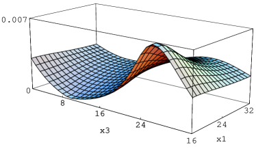
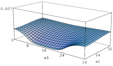
(a)	(b)

Figure 7: Space-space plots of the modulus of the lowest eigenstate for a large caloron on a $32^{3}\cdot 4$ lattic, with (a) periodic and (b) intermediate boundary condition.

In order to clarify how finite volume effects influence these findings, we have doubled both the spatial extension of the lattice and the size of the caloron, which now has its constituents at $x_{1}=x_{2}=16$, $x_{3}=8$ and $25$. The lowest eigenstate with periodic boundary condition, shown in Fig. 7 (a), has a slightly more pronounced maximum, still shifted, to $x_{3}=26$. Around the maximum the modulus is actually close to spherically symmetric as expected since the constituents are quite well separated compared to the typical scale $N_{4}=4$. The minimum is shifted as well, namely to $x_{3}=10$.

This configuration also clarifies the behaviour of the minimum under the change of boundary conditions. Fig. 7 (b) shows that for an intermediate boundary condition the minimum extends to a valley between the minimum locations corresponding to the periodic and antiperiodic modes, respectively.

It is instructive to see how the lowest Laplacian eigenmode looks like in the background of a smaller caloron. The configuration that we employ for this demonstration has only one lump of action density, but the typical dipole behaviour of the Polyakov loop, the latter being close to $-\Eins_{2}$ at $x_{3}=15$ and close to $\Eins_{2}$ at $x_{3}=18$. The modulus of the lowest Laplacian eigenmode has a strong gradient at the location of the lump, too, see Fig. 8 (a). As a matter of fact, the minimum ($x_{3}=15$) reflects the Polyakov loop minimum quite well, while the maximum ($x_{3}=23$) is shifted far outwards.

The maximum is also less pronounced compared to the one of the large caloron. Actually all the presented profiles of the lowest Laplacian eigenmodes away from the monopoles become close to the value an entirely constant mode would have on the corresponding lattice (0.0078 for $16^{3}\cdot 4$, 0.0028 for $32^{3}\cdot 4$). Therefore, the Laplacian modes should be viewed as a wave with local modifications rather than a localized state. The rationale behind that might be the absence of an effective mass that would localize the modes exponentially. For the fermion zero modes this role is played by (the difference of the boundary condition and) the eigenvalues of the holonomy.

Moreover, the maximum of the Laplacian mode is almost static, even for the small ‘instanton-like’ caloron, as can be seen in Fig. 8 (b). The minimum, on the other hand, shows up in a particular time-slice, exactly where the action density is maximal. This is another sign that, from a practical point of view, the use of the minimum is superior compared to the maximum when looking for small calorons (or instantons). The time dependence of the minimum becomes much weaker for large calorons as we have observed (but not shown here), reflecting the more static character of the solution. In the continuum, Laplacian eigenmodes in nontrivial backgrounds will have a zero of topological origin, like fermions do [25].

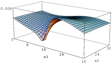
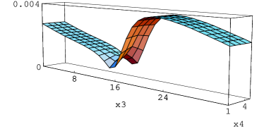
(a)	(b)

Figure 8: (a) Space-space and (b) space-time plot of the modulus of the lowest eigenstate with periodic boundary conditions on the background of a small caloron on a $32^{3}\cdot 4$ lattice.

To summarize, the assignment of a maximum and a minimum in the modulus of the lowest Laplacian eigenmode to the constituents in a caloron is similar to the behaviour of the fermion zero mode. Yet the profile is less localized and shifted. For small calorons it is recommendable to use the minimum, as it was done in Ref. [33], to find instantons on the lattice (in the continuum, the coincidence of the minimum with the instanton center was shown analytically in [34]). The shift observed in that reference nicely agrees with our findings.

By inspecting the components of the Laplacian modes one finds signatures of the Taubes winding. We plot the real and imaginary part of $\phi^{a=1,2}_{\zeta=0}$ in Fig. 9, showing the time dependence at both monopoles. At one monopole core the components are fully static, Fig. 9 (b). At the other monopole, carrying the Taubes winding, they oscillate over one period, however, they seem to contain an additional constant part, Fig. 9 (a).

(a)	(b)

Figure 9: Components of the lowest eigenstate with periodic boundary conditions, in both the fundamental (full lines, real and imaginary part of both components) and the adjoint representation (dashed line, the $\tau_{3}$-component as dotted line), as function of $x_{4}$ at (a) the point $x_{1}=x_{2}=16$, $x_{3}=8$ showing the Taubes winding and (b) the point $x_{1}=x_{2}=16$, $x_{3}=25$ (no winding). Two pairs of lines fall on top of each other in plot (b): real and imaginary part of the second fundamental component and the first two adjoint components.

The general picture of Laplacian modes described so far passes over to the caloron examples of charge $Q=2$. The periodic and antiperiodic modes possess maxima and minima near the corresponding constituents. However, the ring structure in the action density of two overlapping like-charge monopoles is not resolved by the Laplacian modes, in contrast to the fermion zero modes.

3.3 Adjoint representation

In this subsection we discuss (in short) the properties of the lowest Laplacian eigenmode in the adjoint representation. In the Laplacian, the fundamental links $U_{\mu}^{ab}(x)$ are simply replaced by the adjoint ones ${\rm tr}(\sigma^{A}U_{\mu}(x)\sigma^{B}U_{\mu}^{\dagger}(x))/2$ with indices $A,\,B$ running from 1 to 3. The eigenfunctions $\phi_{n}^{A}(x)$ are real in this representation and so there is no continuous phase available to modify the boundary conditions as this was possible in the fundamental representation, Eq. (3) and (4). Nevertheless, we have included the possibility of antiperiodic boundary conditions in the computations.

In caloron backgrounds we basically reproduce the findings of [35], namely that the constituent monopoles are localized by minima in the modulus of the lowest-lying adjoint Laplacian eigenmode with periodic boundary condition. In other words, the single adjoint mode ‘sees’ monopoles of both kinds simultaneously. As Fig. 10 shows, these minima have no shift problems and start to join for a small caloron. That the lowest adjoint Laplacian eigenmode on an instanton background has a zero of second order at the instanton location has been shown in the continuum in [34]. Zeroes in this mode underly the construction of Abelian projected monopoles in the Laplacian Abelian gauge [36]. Thus, for calorons these monopoles coincide with the (gauge independent) constituent monopoles.

Figure 10: The lowest adjoint eigenmodes (with periodic boundary condition) for the large and the small caloron on a $32^{3}\cdot 4$ lattice. The dashed line shows the lowest adjoint eigenmode with antiperiodic boundary condition for the large caloron.

(a)	(b)

Figure 11: The semiclassical configuration described in the text: (a) isosurfaces of the topological density (positive as dark green, negative as light red), (b) isosurfaces locating the minima of the modulus of the lowest adjoint modes, both for periodic (pointlike, balls corresponding to the constituents seen in (a)) and antiperiodic boundary conditions (one-dimensional network).

The lowest adjoint Laplacian eigenmode with antiperiodic boundary condition develops an extended static zero sheet between the monopoles (similar to the lowest fundamental eigenmode with intermediate boundary conditions). The corresponding profile is shown in Fig. 10 as a dashed line.

This feature can be of interest for detection purposes, too. In order to illustrate this, we have investigated a semiclassical case. The gauge field configuration has been obtained by cooling down to a plateau with an action of 1.92 instanton units and a topological charge of $-1$ [31]. As has been described in that reference, there are one selfdual and three antiselfdual monopoles, distinguished by color in Fig. 11 (a). The Polyakov loop at one of the cores is found close to $\Eins_{2}$ and close to $-\Eins_{2}$ at the three others. Isosurfaces (at small value) of the modulus of the lowest adjoint Laplacian eigenmode with either boundary condition are shown in Fig. 11 (b). As for the simple (dissociated) caloron, the periodic mode has static minima at the monopole locations, whereas the regions of small modulus of the lowest antiperiodic mode form a network connecting them.

The lowest adjoint Laplacian eigenmode with periodic boundary condition actually reveals the Taubes winding in a very clear manner, cf. Fig. 9. At the ‘rotating’ monopole (a) the $\tau_{1}$ and $\tau_{2}$ components rotate around the holonomy subgroup generated by $\tau_{3}$, whereas at the other monopole (b) all components are static. For the antiperiodic lowest mode all components perform half a rotation everywhere (to account for the antiperiodicity) with the $\tau_{3}$-component being suppressed.

4 Hopping of the lowest Laplacian mode for thermalized configurations

In the last section we have shown that the lowest Laplacian eigenmodes (fundamental and adjoint) reflect certain properties of smooth classical gauge field backgrounds. Now we explore these modes as an analyzing tool for thermalized gauge field configurations and concentrate on how the dependence on boundary conditions gives additional information.

As a set of thermalized background configurations we take an ensemble of 50 configurations on a $16^{3}\cdot 4$ lattice, generated by Monte Carlo heat bath sampling with the Wilson action at $\beta=2.2$. It represents the confining phase at finite temperature, namely at $T\simeq 0.75\,T_{c}$ (deduced from $\sigma(0)a^{2}=0.22$ for our $\beta$ [37] and $T_{c}/\sqrt{\sigma(0)}=0.709$ for $SU(2)$ YM theory [38]).

Fig. 12 (a) shows a typical spectral flow of the 15 lowest-lying Laplacian modes with the boundary condition angle $\zeta$. The first outstanding feature to notice is that the eigenvalues themselves are much bigger than for the smooth backgrounds considered so far. This is most naturally ascribed to the ultraviolet noise present in the background. The latter has also removed any remnants of the vacuum (or caloron) band structure in this plot. Still, the typical near-crossing points are present, where again the IPR signals big rearrangements in Fig. 12 (b), see e.g. the behaviour of the second and third mode around $\zeta=0.12$.

(a)	(b)
(c)	(d)

Figure 12: Laplacian modes for a configuration in the confined phase. Plotted over the boundary condition $\zeta$ are (a) the 15 lowest-lying eigenvalues in lattice units, (b) the IPR of the 6 lowest-lying modes (with corresponding symbols); (c) the value of the modulus of the lowest eigenmode at its global maximum and minimum (multiplied by a factor 100), (d) coordinates of the global maximum of that mode, displaying the typical $\zeta$-intervals.

Inspecting several independent configurations in the confined phase, the lowest eigenvalue takes on its smallest value around $\zeta=1/4$ (in this respect the configuration in Fig. 12 is not a typical one). This reflects the fact that the average Polyakov loop is close to traceless. On the contrary, in the deconfined phase all low-lying eigenvalues become minimal very close to $\zeta=0$ (and are much bigger at $\zeta=1/2$) with the spectrum grossly similar to Fig. 2 (b), in accordance with the asymmetric Polyakov loop distribution in that phase.

The main observation in the context of Laplacian modes for thermalized backgrounds is the effect of ‘hopping’ of these modes with changing $\zeta$. The IPR of the lowest mode already gives a hint on the existence of what we will call the ‘$\zeta$-intervals’. In the example of Fig. 12 (b) there are three such intervals, inbetween which the IPR has a minimum. It means that the lowest mode delocalizes there in order to rearrange itself. This is confirmed by the inspection of the global maximum in Fig. 12 (c): the value of the modulus at the maximum is minimal at the two transition points $\zeta=0.300$ and $\zeta=0.415$. The main feature of the $\zeta$-intervals is the pinning down of the lowest mode to particular locations. That means that the coordinates of the global maximum have constant values within the $\zeta$-intervals and jump at the transition points, as it is clearly visible in Fig. 12 (d).

For some configurations we have observed two distinct minima in the lowest eigenvalue as a function of $\zeta$, which turned out to be another signal for the existence of the $\zeta$-intervals.

Figure 13: Statistics of the spatial distance of jumps from 50 thermalized configurations (160 jumps occured with spatial distance between 1 and 2 lattice spacings but were not considered further).

In the configuration discussed above the global maximum jumps over spatial distances of 8.5 and 12.7. We will restrict ourselves for the moment to a spatial analysis, since the Laplacian modes are almost static (see below and Fig. 16). We have inspected 50 configurations with 31 boundary conditions and recorded the spatial jumps. Most of them (160) are smaller than two lattice spacings, which can be viewed as a discretization error, where coordinates of the maximum change by one lattice spacing. We have not considered these minimal jumps further.

There remained 120 jumps over at least two lattice spacings. Their distribution is plotted in Fig. 13. It is still dominated by small jumps, however, the jump distance also reaches values almost as high as the maximally possible distance $13.9=(16/2\cdot\sqrt{3})$. There seems to be no correlation of this distance to the $\zeta$-value at which the jump occurs. Instead, the fact that the jump distribution is rather flat around half the linear extension of the lattice (here 8), may point to a random distribution of pinning centres, as suggested for the hopping of fermions in [14]. In order to make such a statement more precise, one would need a model also for the small jumps.

Having underlying calorons in mind, small jumps would be related to small calorons (and larger calorons might actually be suppressed in the same way as large instantons). However, calorons of holonomy close to maximally nontrivial (as expected for the confined phase) would prefer one jump at $\zeta\simeq 1/4$. On the other hand, out of the 50 thermalized configurations we find only 11 configurations with only one jump, but 16 with two, 15 with three and 8 with even four jumps, respectively, and the jumps are scattered between $\zeta=0$ and $\zeta=1/2$.

In the last section we have argued that actually the minima of the modulus of the lowest Laplacian mode are good markers for classical topological objects. In the thermalized background, however, the global minimum is not as stable as the global maximum. Fig. 12 (c) shows that for our example its value is changing smoothly only in a certain fraction of the first $\zeta$-interval. For most values of $\zeta$ the value is highly fluctuating and so is the location (not shown). Furthermore, the number of local minima is typically an order of magnitude bigger than the number of local maxima. Therefore, it is difficult to employ those minima to eventually localize background instantons or calorons within a thermalized gauge field.

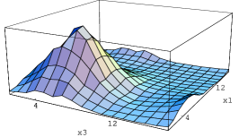
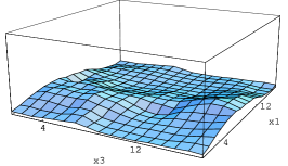
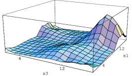
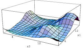
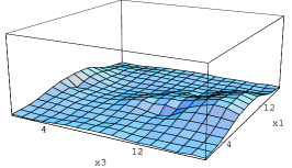
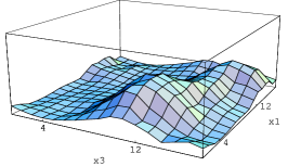
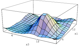
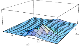
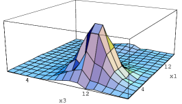
Figure 14: ‘Hopping’ of the modulus of the lowest Laplacian eigenmode. The rows represent different modes. First row: periodic adjoint mode; second to fourth row: fundamental mode with $\zeta=0.020$, $0.355$ and $\zeta=0.480$ representing the three $\zeta$-intervals; fifth row: antiperiodic adjoint mode. The columns show different planes through the lattice. Left: plane through $(x_{2},x_{4})=(12,1)$ with the maximum at $(x_{1},x_{3})=(6,6)$ occurring in the first interval as seen in the second row; middle: plane through $(x_{2},x_{4})=(4,4)$ with the maximum at $(x_{1},x_{3})=(14,14)$ occurring in the second interval as seen in the third row; right: plane through $(x_{2},x_{4})=(6,3)$ with the maximum at $(x_{1},x_{3})=(6,11)$ occurring in the third interval as seen in the fourth row; such that the plots contain the respective global maximum. The vertical scale is 0.1 for the adjoint and 0.05 for the fundamental plots, respectively.

In Fig. 14 we inspect the lowest mode locally. As can be seen immediately, the modulus of the lowest mode is quite smooth which justifies the expectation that these modes do not possess UV fluctuations. Horizontally in the figure we have plotted three lattice planes that contain the locations of the global maximum taken in the different $\zeta$ intervals. The precise $\zeta$-values representing the intervals are chosen by the demand for a maximal IPR. Following the maxima one can see that they either remain as local maxima or disappear in the other $\zeta$-intervals. In other words, the hopping effect comes about by local maxima turning into global ones in particular $\zeta$-intervals, as visualized in Fig. 15.

For comparison we show in the first and fifth row of Fig. 14 the lowest adjoint mode with periodic and antiperiodic boundary condition, respectively. These modes are correlated to the fundamental ones with the closest boundary conditions. Hence the adjoint Laplacian modes are also subject to hopping (when one allows for antiperiodic boundary conditions).

Figure 15: Value and location ($\pm$ one lattice spacing) of all local maxima that become global ones in some $\zeta$-intervals.

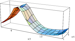
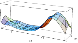
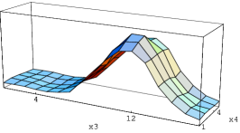
Figure 16: Time dependence of the maxima in the three intervals, i.e. at $\zeta=0.020$, $\zeta=0.355$ and $\zeta=0.480$ with $(x_{1},x_{2})=(6,12)$, $(x_{1},x_{2})=(14,4)$ and $(x_{1},x_{2})=(6,6)$, from left to right, respectively. The vertical scale is 0.05 as in the corresponding space-space plots of Fig. 14.

When compared to the classical backgrounds the maxima in thermalized backgrounds are more pronounced, i.e. more localized (compare the scales in Fig. 12 (c) and Fig. 6). Accordingly, the IPR’s are higher, varying between $I=4$ and $I=11$ for the lowest fundamental mode (cf. Fig. 12 (b)). Moreover, the regions outside the lumps have now a lower modulus. This can be quantified by the average of $|\phi|$, which for the thermalized background is lower than the classical one (and rises at the points of transition). For the lowest adjoint mode the IPR is even higher, $I=21$ and $I=53$ for periodic and antiperiodic, respectively, an effect which has already been observed in [17].

Thus, the overall behaviour of the lowest Laplacian eigenmodes in equilibrium background fields is again analogous to the behaviour of fermionic zero modes [8]. Still the lowest Laplacian mode seems to be broader than the fermionic counterpart, which is probably also the reason why the maxima are quite static, see Fig. 16.

(a)	(b)	(c)
(d)	(e)

Figure 17: Characterization of the cluster(s) occupied by Laplacian modes: accumulated norm (smooth curve) together with the relative size (step curve) as a function of the space-time filling fraction of the mode. The upper row shows (a) the lowest fundamental Laplacian mode with $\zeta$ inside the first interval (the mode is localized), (b) at the first transition (where it has turned to global) and (c) inside the second interval (less global). The lower row shows the lowest adjoint Laplacian mode with (d) periodic boundary condition and (e) antiperiodic boundary condition (both are highly localized).

At this point it is desirable to discuss more quantitatively the feature of localization of the Laplacian modes. We have found it useful to add to the IPR measurements done so far a description suggested by Horvath [39]. It compares how quickly clusters (in our case of large modulus of the Laplacian mode) grow in size and how much – at the same time – they gain in norm, when their total volume increases by lowering the lower cutoff in the cluster definition. The size of the cluster has been defined here as the diagonal of the enclosing 3D cube (since the modes are almost static) and then divided by the diagonal of the 3D lattice. According to this description, a profile is called localized when small clusters already accumulate a large norm fraction.

For the Laplacian modes we find mostly one big cluster. As Fig. 17 shows, the adjoint modes are always local, but the fundamental modes are sometimes rather global, depending on the boundary condition $\zeta$. This is the case for instance for $\zeta=0.300$ (first transition point) and $\zeta=0.355$ (second $\zeta$-interval), cf. Fig. 17 (b) and (c). There the cluster has already its maximal size, i.e. has percolated through the lattice, although the accumulated norm is around three quarters only.

Thus this analysis supports the view of Laplacian modes being close to wave-like (as has already been argued in the caloron background). Hence they should be able to reflect the background gauge field quite well everywhere on the lattice. This is an advantage for Laplacian gauge fixing and the filter method proposed in the next section.

To end this section about Laplacian modes in equilibrium backgrounds, we want to mention a possibility to connect the behaviour of Laplacian modes in thermalized and classical backgrounds. It involves the smoothing of the gauge field background by applying smearing (for instance 5 steps) to it. Then the maximum decreases in modulus (and can move or join with local maxima), whereas the minimum value increases. More importantly, the number of local minima decreases drastically and from some stage on it should be possible to use the minima as markers of the (gradually emerging) topological structure. However, such an approach mixes two techniques to suppress UV fluctuations and it would be cleaner to interpret directly the Laplacian modes of the original configuration.

(a)	(b)

Figure 18: Scatterplots of the Polyakov loop (horizontal) at lattice sites where the modulus of the Laplacian modes (vertical) with $\zeta=0.02$ (close to periodic, crosses) and $\zeta=0.48$ (close to antiperiodic, circles) is large: (a) for the original configuration and (b) for the Polyakov loop measured on the configuration with 5 smearing steps applied.

(a)	(b)

Figure 19: Comparison of contours of constant Polyakov loop (dashed curves) after smearing and of the unsmeared Laplacian modes at large modulus (70% and 90% of the maximum, full curves), in lattice planes where the latter become maximal. (a) the periodic mode vs. positive Polyakov loop (0.7 and 0.9) in $(x_{2},x_{4})=(12,1)$, (b) the antiperiodic mode vs. negative Polyakov loop ($-0.7$ and $-0.9$) in $(x_{2},x_{4})=(6,3)$.

Interestingly, we have found an interrelation of the pinning of the Laplacian modes to a gluonic observable, namely the Polyakov loop. The maximum of the modulus of the periodic mode is correlated to a positive Polyakov loop, whereas the maximum of the antiperiodic mode prefers negative values, see Fig. 18 (a). Of course, this expresses only an overall tendency, because there is a mismatch between the smoothness of the Laplacian mode and the roughness of the Polyakov loop. To make this statement quantitative one can measure the sum over the Polyakov loop weighted with $|\phi|^{2}$ of the periodic and antiperiodic mode (the horizontal coordinate of the ‘center of mass’ of that figure). This gives weighted averages of 0.206 and $-0.1154$ for the two cases, respectively, while the ordinary Polyakov loop average is 0.005.

We have smeared the gauge field which results also in smoothing the Polyakov loop, then we compared the latter to the Laplacian modes of the original configuration. The mentioned tendency becomes more pronounced, see Fig. 18 (b) and is now locally visible. As Fig. 19 shows, the smeared Polyakov loop provides a collection of pinning centres for the modes to settle down at Polyakov loops near $\Eins_{2}$ and $-\Eins_{2}$, repectively. Hence the Laplacian modes on the unsmeared configuration know about the Polyakov loop landscape, which only emerges after smearing.

The direction of this correlation agrees with the findings in classical solutions (compare Fig. 1 (a) and Fig. 6) which seems to suggest calorons as ‘underlying’ the thermalized gauge fields. However, it can also be interpreted within the Anderson localization scenario, with the Polakov loop localizing the candidate ‘minima of a random potential’ to be occupied by the scalar or fermionic modes.

5 A new filter method

In the following we will introduce a new low-pass filter based on the Laplacian modes. It uses an exact representation of the links in the form of a sum of the latter, which, by truncation, should remove UV noise and find the ‘underlying IR structures’. Hence, the spirit of our method is close to a Fourier decomposition or a (gauge invariant) high momentum cut-off.

Technically, our approach is similar to the one in [18], where the field strength was given in terms of a sum over fermionic modes. A similar mode truncation for the overlap-based topological charge has been used in [40] and studied in more detail in [41, 42]. However, we will obtain directly the link variables and in this ‘reconstructed’ configuration any observable can be measured.

5.1 Derivation and properties

We combine the definition of the gauge covariant Laplace operator, Eq. (1), with a decomposition into its eigenmodes:

$$-\triangle^{ab}_{xy}=\sum_{n=1}^{\mathcal{N}}\lambda_{n,\zeta}\phi^{a}_{n,\zeta}(x)\phi^{*b}_{n,\zeta}(y)$$ (11)

At $y=x+\hat{\mu}$ one immediately obtains

$$U_{\mu}^{ab}(x)=-\sum_{n=1}^{\mathcal{N}}\lambda_{n,\zeta}\phi^{a}_{n,\zeta}(x)\phi^{*b}_{n,\zeta}(x+\hat{\mu})$$ (12)

The corresponding formula for $U^{\dagger}_{\mu}$ at $y=x-\hat{\mu}$ is fully equivalent to Eq. (12), while

$$\delta^{ab} \!= \!\frac{1}{2}\sum_{n=1}^{\mathcal{N}}\lambda_{n,\zeta}\phi^{a}_{n,\zeta}(x)\phi^{*b}_{n,\zeta}(x)$$ (13)

$$0 \!= \!\sum_{n=1}^{\mathcal{N}}\lambda_{n,\zeta}\phi^{a}_{n,\zeta}(x)\phi^{*b}_{n,\zeta}(y)\qquad\forall y\neq x,x\pm\hat{\mu}$$ (14)

could be used as a check for the approximation to be discussed now. Notice that the eigenfunctions enter these expressions in a combination that is invariant under a multiplication of the eigenfunctions with a complex phase. More general, at a level with degeneracy $k$ the expressions are invariant under a change of the basis (a global $U(k)$ rotation acting on the index $n$).

The idea of the filter is to truncate the sum in Eq. (12) at a rather small number $N$ of eigenmodes. When doing so, the question arises, how to relate the r.h.s. of Eq. (12) to a unitary link variable. We remind the reader that in the cooling method staples are added. This gives a quaternion, which becomes an element of $SU(2)$ upon multiplying by a real number. We will use the same projection. However, the non-trivial task here will be to arrive at a quaternion in the first place. We will show now that the charge conjugation symmetry of the Laplacian helps to resolve this issue.

For the $\phi$-terms in the sum we use the abbreviation

$$u_{\mu}^{ab}(x)_{n,\zeta}=\phi^{a}_{n,\zeta}(x)\phi^{*b}_{n,\zeta}(x+\hat{\mu})\,.$$ (15)

The charge conjugation symmetry (5) implies

$$u_{\mu}^{\prime}(x)_{n,-\zeta}=\epsilon\,u_{\mu}(x)_{n,\zeta}^{*}\,\epsilon^{-1}\,,\qquad\epsilon=i\sigma_{2}\,.$$ (16)

For $\zeta=0$ (periodic) and $\zeta=1/2$ (antiperiodic) these contributions are automatically included in the sum in Eq. (12) (as every level is two-fold degenerate with eigenmodes $\phi$ and $\phi^{\prime}$). To make use of this relation for general $\zeta$, we take the average of the link formula (12) over $\zeta$ and $-\zeta$

$$U_{\mu}(x) = -\frac{1}{2}\,\sum_{n=1}^{\mathcal{N}}\left[\lambda_{n,\zeta}u_{\mu}(x)_{n,\zeta}+\lambda^{\prime}_{n,-\zeta}u^{\prime}_{\mu}(x)_{n,-\zeta}\right]$$ (17)

$$= -\frac{1}{2}\,\sum_{n=1}^{\mathcal{N}}\lambda_{n,\zeta}\left[u_{\mu}(x)_{n,\zeta}+\epsilon\,u_{\mu}(x)_{n,\zeta}^{*}\,\epsilon^{-1}\right]\,.$$

So far this manipulation is exact, but seems artificial. However, it will help in the truncation of the sum. Parametrising the matrix in the bracket we have

$$\left(\begin{array}[]{cc}a&b\\ c&d\end{array}\right)+\left(\begin{array}[]{cc}d^{*}&-c^{*}\\ -b^{*}&a^{*}\end{array}\right)=\left(\begin{array}[]{cc}u&v\\ -v^{*}&u^{*}\end{array}\right)$$ (24)

For a matrix of this form the inverse is the same as the hermitean conjugate up to a factor, which is the determinant $|u|^{2}+|v|^{2}$ and positive for all practical purposes. Hence, the matrix obtained by truncating the sum is an element of $SU(2)$ up to the square root of the determinant by which we will divide.

An alternative way to arrive at a unitary link is to use the unitary matrix in the singular value or polar decomposition. It agrees with our procedure under special circumstances, for instance if the matrix to start with has a real determinant as is the case for $\zeta=0$ and $\zeta=1/2$. In our point of view the inclusion of both $\zeta$ and $-\zeta$ is very natural since these boundary conditions contain the same information of the Laplacian mode (same eigenvalue and charge conjugated eigenmode).

To summarize, there is an exact formula for the link variables in terms of the Laplacian modes, namely Eq. (17). It is this sum we truncate to obtain the filtered links

$$\tilde{U}_{\mu}(x)_{N,\zeta}=\left(-\sum_{n=1}^{N}\lambda_{n,\zeta}\left[u_{\mu}(x)_{n,\zeta}+\epsilon\,u_{\mu}(x)_{n,\zeta}^{*}\,\epsilon^{-1}\right]\right)_{{\rm det}=1}\quad M_{{\rm det}=1}\equiv M/\sqrt{{\rm det}\,M}\,,$$ (25)

where the operation $(\ldots)_{{\rm det}=1}$ forces the link variable to have unit determinant (and we have dropped the factor $1/2$).

Eq. (25) is our final proposal for a low-pass filter acting on lattice configurations. It is a mapping from the original links $U_{\mu}(x)$ to the filtered ones $\tilde{U}_{\mu}(x)_{N,\zeta}$ via the Laplacian eigenmodes with the phase $\zeta$ in the boundary condition as a free parameter. The quality of the filter is controlled by $N$, where $N=\mathcal{N}$ reproduces the original configuration exactly (with no determinant correction necessary). Formally, the filtered links $\tilde{U}_{\mu}(x)$ look like composite fields, as they are produced by bilinears in $\phi$, Eq. (15).

Our approximation keeps the full gauge covariance, because if a gauge transformation $g(x)$ acts on $\phi(x)$ from the left, then $g^{\dagger}(x+\hat{\mu})$ acts on $\phi^{*}(x+\hat{\mu})$ from the right (and the determinant is gauge invariant) resulting in $g(x)\tilde{U}_{\mu}(x)g^{\dagger}(x+\hat{\mu})$ as it should be.

It is instructive to investigate the extreme case of $N=1$, i.e. the contribution from the lowest mode only. Then the filter gives – independent of the starting configuration – a pure gauge $\tilde{U}_{\mu}(x)$, but with a Polyakov loop given by $\zeta$.

The best way to understand this is going into Laplacian gauge [16]. That is to rotate the lowest mode to have only an upper nonvanishing component, which is real. Then the matrices $u_{\mu}(x)$ would have only a real 11-component and adding the charge conjugate and normalising by the square root of the determinant makes all $\tilde{U}_{\mu}(x)$ equal to the identity. However, for the nontrivial boundary conditions of Eq. (3) one has to slightly rethink this procedure. The simplest way to define the gauge fixing then is to demand the form $({\rm real},\,0)^{T}$ for the (always periodic) $\varphi_{\zeta}(x)$. By transforming back to $\phi_{\zeta}(x)$, Eq. (4), and plugging this into Eq. (15) the same considerations hold, with the only exception that $u_{\mu=4}^{a=b=1}(x)$ receives an additional factor $\exp(-2\pi i\zeta/N_{4})$. After charge conjugation and normalising the filtered links become $\tilde{U}_{4}(x)=\exp(-2\pi i\zeta\tau_{3}/N_{4})$. Hence the filtered Polyakov loop is

$$\frac{{\rm tr}}{2}\,\tilde{\mathcal{P}}(\vec{x})_{N=1,\zeta}=\cos(2\pi\zeta)\quad\forall\vec{x}\,.$$ (26)

These considerations did not use that $\phi(x)$ is the ground state. Thus every eigenmode alone gives vanishing action and a Polyakov loop as above. Since the superposition in Eq. (25) is nonlinear, we expect $N=2$ to be the first nontrivial filter with nonvanishing action. As we will see in the next section, the trace of the Polyakov loop will start to fluctuate in this case, but on average is still close to the value of Eq. (26).

Let us add a few remarks on the possible stability of the filtered links $\tilde{U}_{\mu}(x)_{N,\zeta}$ under variations of $N$. From the normalization of $\phi_{n}(x)$ follows that the entries of $u_{\mu}(x)$ are roughly $O(1/\mathcal{N})$. The prefactor $\lambda_{n}$ is rising slightly with $n$, such that one can expect the terms in the sum to be of the same order of magnitude.

The only exception to this argument is the caloron background at $\zeta=1/4$, where the lowest Laplacian eigenvalue is strongly suppressed w.r.t. the other eigenvalues. As a result, the lowest mode practically does not contribute to the filtered links. Here the situation is analogous to the fermionic filter in [18], where the zero mode does not contribute.

Actually, the staggered symmetry of the Laplacian can be used to improve the convergence. Relation (6) between low and high modes immediately gives

$$u_{\mu}^{\prime\prime}(x)_{\mathcal{N}-n,\zeta}=-u_{\mu}(x)_{n,\zeta}\,.$$ (27)

Therefore, the inclusion of the upper end of the spectrum does not change the contributions to the filtered links locally. It only reweights the terms in the sum (25)

$$-\lambda_{n}\rightarrow 4D-2\lambda_{n}\,.$$ (28)

With this insertion one has to sum in Eq. (25) only over half the spectrum to obtain the original link. Now each subsequent term $u_{\mu}(x)_{n}$ has a smaller weight. In particular, the weight of the ground state is the biggest.

The price to pay is to include the upper end of the spectrum of the Laplacian, which a priori contradicts the meaning of a low-pass filter. We decided not to include the highest modes and to stick to Eq. (25). Nevertheless, we have checked the consequences of such a modification for the results presented below. The changes are quite small apart from the case of reconstructing the caloron background from $N=2$ modes at $\zeta=1/4$, the case discussed above. Therefore, it seems that the local information $u_{\mu}(x)_{n}$ is more important for the filtered links than the relative weights $\lambda_{n}$ of the eigenfunctions. One might speculate whether eigenmodes other than the lowest ones could be used and whether the weights could be chosen arbitrarily (constant or random).

5.2 Classical objects seen through the filter

In this subsection we test the filter in a controlled environment, namely for calorons as smooth configurations.

First we want to study a technical detail, namely how big the determinant is that appears in (25) to scale up the sum to an $SU(2)$-valued link. In other words, how much of the link is captured by the superposition of a finite number of modes (in a naive sense without inspecting any structure in the links).

$N$	1	4	10	50	200
min${}_{x}\,\log_{10}$ det	$-15.3$	$-12.1$	$-8.5$	$-6.1$	$-4.1$
max${}_{x}\,\log_{10}$ det	$-11.9$	$-8.6$	$-7.6$	$-5.5$	$-3.9$

Table 1: Behaviour of the determinant used to project to an $SU(2)$-element in the truncated sum (25), depending on the number $N$ of modes. The background is the large caloron on $16^{3}\cdot 4$ with $\zeta=1/4$.

From Tab. 1 one can read off that this determinant is small (the correction factor is large) when only a few modes are taken. This is to be expected from the smallness of the $\phi_{n}(x)$ that are square-normalized on the entire lattice. The determinant grows with $N$. Of more relevance is that the minimum and the maximum of the determinant taken over the lattice approach each other, such that all links appear ‘equally well filtered’.

The most important question in the caloron context is whether the filtered links produce the action density lumps of the two constituent monopoles including the typical structure in the Polyakov loop. In Fig. 20 we give the observables corresponding to Fig. 1 (a) in the filtered configuration with different $\zeta$ and $N$.

For the chosen $N\ll\mathcal{N}$, the boundary condition parameter governs the average Polyakov loop. In the intermediate case $\zeta=1/4$ the average Polyakov loop trace is 0 with extrema of nearly $\pm 1$ at the monopole cores, see Fig. 20 (b). In the periodic case $\zeta=0$ the Polyakov loop is almost everywhere $\Eins_{2}$ with a dip resembling $\mathcal{P}=-\Eins_{2}$ at the corresponding monopole, see Fig. 20 (a). The antiperiodic case (not shown) is complementary, $\mathcal{P}\simeq-\Eins_{2}$ with a signal at the other monopole.

(a)	(b)	(c)

Figure 20: Action density, topological density and Polyakov loop computed from filtered links in the background of the large caloron of Fig. 1. (b) $\zeta=1/4$ with $N=4$ modes (action and topological density multiplied by 100); (c) more modes $N=150$ (scale 400 just as in the original plot Fig. 1 (a)). (a) periodic boundary condition $\zeta=0$ with $N=4$ modes (scale 30).

This picture stays the same when more modes are taken into account. The Polyakov loop for the periodic case develops a stronger dip then, but is still very close to $\Eins_{2}$ anywhere else. For the intermediate case the average stays close to 0. Locally it agrees almost perfectly with the one of the original configuration, see Fig. 20 (c) for $N=150$ vs. Fig. 1 (a). To make this more quantitative we give the values of the Polyakov loop at the action density lumps (see below) and on average in Tab. 2.

$N$	4	10	100	150	200	original
$x_{3}$ at lumps	4.0	3.7	4.1	4.3	3.7	4.4
	13.0	13.3	12.9	12.8	13.3	12.6
action density	0.014	0.010	0.0023	0.0037	0.0026	0.0032
top. density	0.013	0.010	0.0019	0.0035	0.0026	0.0032
Pol. loop	$\pm\,$0.84	$\pm\,$0.80	$\pm\,$1.00	$\pm\,$0.99	$\pm\,$0.99	$\pm\,$0.97
total action	2.4	2.2	1.62	1.34	1.63	1.07
total top. charge	0.98	0.99	1.00	1.00	1.00	1.00
average Pol. loop	$-2\cdot 10^{-6}$	$-4\cdot 10^{-6}$	$-0.02$	$0.0001$	$-0.0002$	$-0.0003$

Table 2: Quality of the reconstruction of a large caloron from the filter with different number of modes. Both, local quantities (interpolated) and global quantities converge to the original values within some error margin.

The findings for the reconstructed action and topological charge are analogous. In order to compare the two, we have computed them with the help of an $O(a^{4})$ improved field strength tensor [43]. The periodic case sees only one monopole, while the intermediate case is able to detect both (Fig. 20). We conclude that the boundary condition $\zeta=1/4$ is the appropriate one when one wants to describe calorons with maximally nontrivial holonomy through the filter, as is also clear from the discussion of the contribution of a single mode in the last section.

Remarkably, the filter with the number of modes as low as $N=4$ already has quite some knowledge about the classical structures. Although the action density lumps are a bit spiky and their locations are not perfect as recorded in Tab. 2 (notice also the different scales for the action and topological density used in Fig. 20 (b) vs. (c) and Fig. 1 (a)), they clearly reflect the constituent structure with opposite Polyakov loops. The two lumps are almost selfdual (cf. third and fourth row in Tab. 2). Furthermore, the adopted definition of the topological charge works quite well for the filtered links and gives a total topological charge close to 1. We stress that the filtered configurations have not undergone further cooling and their approximate selfduality is a remnant of the original configuration passed on by its lowest-lying Laplacian modes.

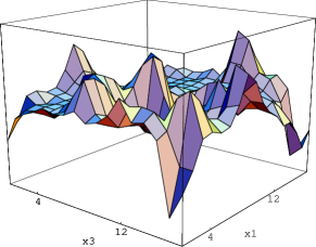
(a)		(b)
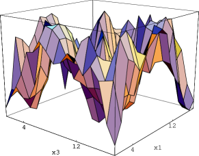
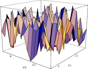
(c)		(d)

Figure 21: Polyakov loop ‘evolution’ with increasing number $N$ of modes for a thermalized configuration in a fixed lattice plane (the one of Fig. 25). (a) $N=2$, (b) $N=10$, (c) $N=100$ and (d) the original configuration. The vertical axes are from $-1$ to $1$.

The inaccuracies of the $N=4$ case are cured by increasing the number $N$ of modes used in the filter, however, not systematically. The quite perfect case $N=150$ used for the plot in Fig. 20 (c) is contrasted by $N=200$, where some of the observables are further away from the original configuration. We interpret this as a limitation on the precision of the filter. Away from the ultimately exact limit $N=\mathcal{N}$, the filter will reproduce the classical background only within some error and hence it is not useful to take more than a few hundred modes into account (at least for this example). This does not spoil the use of the filter at all, since its intended application will be mainly to thermalized configurations (see below). There it is not the aim to reproduce the rough background to a high precision, but to keep only a minimal structure of it such that it still captures the physical randomness.

We note in passing that the Taubes winding inside caloron configurations as well as the ring structure for the charge 2 example are displayed by the filtered configurations, too.

5.3 Are the filtered fields confining?

The next two subsections are devoted to the application of the filter to thermalized configurations. One of the main issues here is whether the filtered links still give rise to confinement.

To this end we have measured the Polyakov loop correlator on the ensemble of 50 configurations on a $16^{3}\cdot 4$ lattice created at $\beta=2.2$. The Polyakov loop as the deconfinement order parameter has average $0$ and therefore we choose $\zeta=1/4$ in the construction of the filter, Eq. (25). Indeed, the filtered Polyakov loop $\langle{\rm tr}\,\tilde{\mathcal{P}}/2\rangle$ averaged over the lattice has an expectation value compatible with 0 (with 50 configurations giving standard devitations from 0.015 for $N=2$ to 0.083 for $N=100$ whereas the original standard deviation is 0.025). This again confirms that the average Polyakov loop for small $N$ follows the one of the trivial case $N=1$. In a way, we adapt the Polyakov loop average by a parameter in our filter and then look at correlations in fluctations on top of it.

Fig. 21 shows how the Polyakov loop looks locally (for a fixed configuration and lattice plane). When taking more modes into account, the Polyakov loop deviates further and more often from the average 0. Fig. 22 makes this statement more quantitative. It displays the distribution of Polyakov loops for one filtered configuration. As is clear from the discussion so far, the distribution for $N=2$ is quite narrow and broadens with growing $N$. At $N=100$ it is very close to the one of the original distribution and the Haar measure $\sqrt{1-({\rm tr}\,\mathcal{P}/2)^{2}}$.

Figure 22: Distribution of Polyakov loops over the lattice sites for one configuration when filtered with the intermediate boundary condition $\zeta=1/4$ for $N=2$ (narrow distribution around 0, divided by 15 to fit in the same plot) and $N=100$ (solid line) compared to the orignal configuration (dashed) and the Haar measure (dotted).

Fig. 23 shows the logarithm of the Polyakov loop correlator, related to the interquark potential, measured at the filtered ensembles with $N=2$ to $N=100$ together with the unfiltered one. There is clear evidence that the filtered Polyakov loop correlator decays exponentially with the distance, in roughly the same window as the original one does. The potential after filtering has no sign of a Coulomb regime since the filter has washed out short range fluctuations as it should. The filtered curves are also shifted vertically. The value at zero distance represents the width of the Polyakov loop distribution. It approaches the original one from below, because the filtered distributions are narrower, as was shown in Fig. 22.

In order to cast the confining behaviour into numbers we have performed an exponential fit $c\,\exp(-\bar{\sigma}r)$ in the range between $3$ and $6$ lattice spacings. The slope $\bar{\sigma}$ is directly proportional to the string tension $\sigma=\bar{\sigma}/N_{4}\,a^{2}$. We will use the corresponding string tension of the original configurations as the reference observable. The lower end of the fit region was taken such that the numerical value of $\bar{\sigma}$ for the original configuration is stable when compared with a fit over 1 to 6 lattice spacings including a Coulomb part. Towards large distances the fit was limited by statistical errors. The obtained values for the string tension and estimates of its error are given in Tab. 3. Although the approach of the filtered string tensions for the number of modes between $N=2$ and $100$ to the original one is again not monotonic, the latter is reproduced within 15% (for $N=4$ modes the reproduced string tension is almost perfect).

Figure 23: Polyakov loop correlator plotted on an inverse logarithmic scale over the distance for different $N$ compared to the original one.

Figure 24: Test whether the original and filtered configurations contain correlated fluctuations disordering the Polyakov loop. Correlators $C(r)$ (upper curve) and $C_{\rm ind}(r)$ (lower curve), see text.

A priori it is not obvious whether the Polyakov loop fluctuations in the filtered and the original configurations are correlated or whether the filter creates independent fluctuations (a pointwise scatterplot of the two respective Polyakov loops against each other shows a correlation setting in not below $N=50$ modes). A similar question has been investigated in [45] concerning two Wilson loops $W_{1}(C)$ and $W_{2}(C)$. There the correlation $\langle W_{1}(C)W_{2}(C)\rangle$ (i.e. between different Wilson loops along the same curve $C$) was compared to $\langle W_{1}(C)\rangle\langle W_{2}(C)\rangle$ representing the hypothetic independence of the Wilson loops (and decaying exponentially with the area of $C$). Adopting this idea to our case we have to compare

$$C(|\vec{x}-\vec{y}|) = \frac{1}{16}\,\langle{\rm tr}\,\mathcal{P}(\vec{x}){\rm tr}\,\mathcal{P}(\vec{y})\cdot{\rm tr}\,\tilde{\mathcal{P}}_{N}(\vec{x}){\rm tr}\,\tilde{\mathcal{P}}_{N}(\vec{y})\rangle\qquad{\rm to}$$ (29)

$$C_{{\rm ind}}(|\vec{x}-\vec{y}|) = \frac{1}{16}\,\langle{\rm tr}\,\mathcal{P}(\vec{x}){\rm tr}\,\mathcal{P}(\vec{y})\rangle\langle{\rm tr}\,\tilde{\mathcal{P}}_{N}(\vec{x}){\rm tr}\,\tilde{\mathcal{P}}_{N}(\vec{y})\rangle\,.$$ (30)

We did this for $N=4$ and show in Fig. 24 that the correlator $C(r)$ becomes independent of the distance $r$ rather quickly. $C_{{\rm ind}}(r)$ of course decays exponentially with the sum of the string tensions of the original and the filtered case. We conclude that the fluctuations disordering the Polyakov loop for the original and the filtered configuration are not independent but rather correlated.

5.4 Structures found by the filter

Finally, we give a first description of the vacuum structures that appear when the filter is applied to an individual configuration from an equilibrium ensemble, representing finite temperature in our case.

$N$	2	4	10	50	100	original
$\sigma/10^{5}\,MeV^{2}$	$1.732(31)$	$1.447(25)$	$1.299(17)$	$1.385(13)$	$1.574(25)$	$1.509(70)$
Wilson action	66	84	106	177	234	2131
max. # clusters	37	50	70	79	104	342

Table 3: Observables to characterise the filter when acting on equilibrium configurations. The string tension is computed from 50 configurations, the other two observables are for the example configuration characterised locally in Fig. 21 and 25.

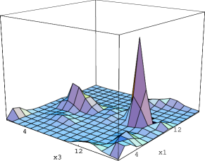
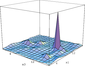
(a)		(b)
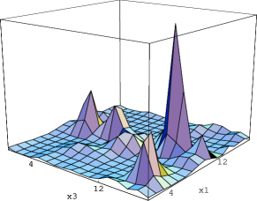
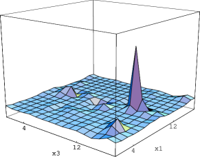
(c)		(d)
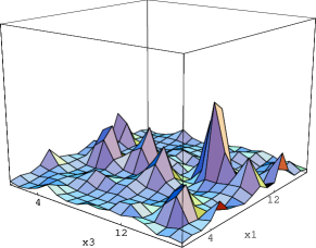
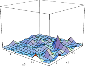
(e)		(f)
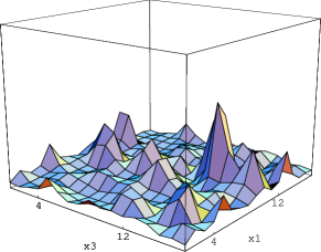
(g)		(h)

Figure 25: Left column: ‘Evolution’ of the action density with growing number of modes in the filter, (a) $N=4$, (c) $N=10$, (e) $N=50$ and (g) $N=100$. Chosen is the lattice plane $(x_{2},x_{4})=(6,4)$ which contains the global maximum for $N=10$ sitting at $(x_{1},x_{3})=(10,13)$. For comparison the action densities for the same configuration after 5 steps of smearing (b), after 2 steps of cooling (f) and for the original configuration (h) are presented with uniform scale. In the second row a comparison is made between the action density (c) and the topological density (d), both after filtering with $N=10$.

The behaviour of the Polyakov loop was shown in the previous section (Fig. 21). The total action of the filtered configuration behaves like $N^{1/3}$ in a range from $N=2$ to $N=100$ eigenmodes. The interpretation of this particular dependence is not obvious, but the overall picture is clear: the more modes are included in the filter, the more fluctuations occur and contribute to the total action. In the example we use (cf. Fig. 21 and 25) the action in the first nontrivial case $N=2$ is 66 in instanton units of $2\pi^{2}$, compared to a total plaquette action of 2131 for the original configuration. The first number should be read as the minimal content that survives the filter. The only way to achieve an ‘even smoother configuration’ would be to apply the filter to the already filtered configuration.

The global maximum of the action density is only weakly varying with $N$, meaning that there are peaks of about the same height at every stage of the filter. From Fig. 25, showing the action density in a fixed lattice plane for different $N$, it is evident that these peaks are quite narrow. This effect is counterintuitive, but has also been observed for caloron backgrounds in the last section. The peaks look the same in a space-time plane, too, i.e. they are not static. The figure also shows that at least some of the peaks are stable w.r.t. $N$, that is they stay as local maxima. Their width is not changing much either.

In order to more quantitatively describe the filtered structure we have performed a cluster analysis. Lowering the threshold we have recorded the number of clusters and their respective volume, size and accumulated action. The number of clusters first raises and after reaching a plateau decreases again due to cluster mergings, while the peaks remain.

As shown in Fig. 26, the corresponding curves fall almost on top of each other, when the number of clusters is taken relative to its maximum at that $N$ (see Tab. 3). That suggests that the difference in the filtered action for different $N$ is due to the different number of clusters. Otherwise they are rather similar. Other indications for that are the volume, the size and the action per cluster, which – plotted as a function of the threshold – fall on top of each other as well.

Figure 26: Relative number of action density clusters as a function of the lower threshold for a filtered configuration at different $N$.

In Tab. 3 we give for each $N$ the maximal number of clusters. The latter appears at a threshold of roughly a third of the global maximum, where all clusters together have accumulated a few percent of the lattice volume and roughly 15% of the action. It is interesting to notice that the maximal number of action density clusters roughly agrees with half the total action (in instanton units, see Tab. 3 third and second row). A lower bound for the estimated action per peak is thus 0.3. More realistic is to assign part of the remaining action below the threshold to the peaks (sitting in their tails). From Fig. 26 we read off that at a threshold of 0.01 (around $1/15$ of the global maximum) the number of clusters starts to fluctuate because the region of action density noise has been reached. At that threshold the accumulated action of the clusters is roughly 60% of the full one. This results in an average action per peak of 1.2 in instanton units. Hence, from an action density point of view, this estimate is compatible with an interpretation of the peaks as (possibly fractional) instanton lumps.

Indeed, the local maxima of the action density are often accompanied by local extrema in the topological charge density. This is visualized for $N=10$ in Fig. 25 (d). However, the topological charge density does not equal the action density at the peaks. For the global maximum at $N=10$ the ratio of both quantities is 0.87, but for other local maxima no signature of (anti)selfduality was found. Moreover, the total topological charge of generic configurations expressed in terms of the filtered links is not close to an integer. In this respect, the configuration, although it is filtered, is not smooth enough to make the $O(a^{4})$ improved field strength definition of the topological charge work. Fermionic definitions via the index should be used to determine whether the filter preserves the total topological charge.

The peaks seem to have nothing to do with the maxima of the modulus of the Laplacian mode in that background, but with the determinant used as the normalization factor in Eq. (25). Obviously this determinant is given in terms of eigenmodes (and eigenvalues) of the Laplacian, too, thus it also contains information about the gauge background.

Another interesting question is whether the new filter is related to smearing and cooling. In Fig. 25 we compare the corresponding action densities to the filtered ones, where the number $N$ of modes was chosen such that the total actions are comparable. For instance, 2 cooling steps result in an action of 172, which therefore compares to $N=50$ (see Fig. 3 second row) and 5 smearing steps result in 84 which compares to $N=4$. As the third and the first row of Fig. 25 show, the corresponding peaks seem to agree locally, which is a nontrivial correlation, because both methods lower the total action by a smoothing procedure, but in completely different ways. In contrast, 5 cooling steps lead to an action of 56, which seems to be comparable to $N=2$. The action density, however, looks very different. It is clear that for more cooling steps the correlation to the filter has to break down, since cooling typically drives towards action plateaus of a few instanton units and finally removes the string tension. This is avoided in the filter method.

More work has to be done to better understand the ($N$-dependent) spiky structures induced by the filter.

6 Discussion and outlook

We have investigated Laplacian eigenmodes in both classical and thermalized gauge configurations with respect to their capability to analyze certain properties of the background. Our localization studies for classical backgrounds lead to the conclusion that there is an analogy to fermionic (near zero) modes. In caloron backgrounds they detect the monopoles by a minimum and a maximum and hop between these constituents upon changing the boundary condition angle $\zeta$. We conclude that such a localization is merely due to information about the gauge background in the covariant derivative, which is modified by the angle $\zeta$ in the same way, and does not depend much on the spin of the analyzing field.

Yet, there is some difference between fermionic and Laplacian modes. This concerns for instance the behaviour under intermediate boundary conditions. For the caloron fermionic zero mode one lump grows at the expense of the other, while the Laplacian ground state develops a valley. Also the precision of the localization is lower than for the fermions: the maximum of the modulus is less pronounced and static even for a time-dependent action density of the background. For the minimum these problems do not occur, but the locations of both, minimum and maximum, deviate from the constituents. Moreover, the modulus of the mode approaches the average value away from those structures and hence the IPR’s are rather small. That is why the Laplacian modes resemble modified waves rather than exponentially localized discrete states (in continuum language).

The wave character also applies to the Laplacian modes in the adjoint representation, where the underlying structures (constituent monopoles or instantons) are detected by minima only. We expect them to become zeros in the continuum, which is natural from the point of view of the Laplacian Abelian projection. For antiperiodic adjoint modes these minima form even two-dimensional sheets between the constituent monopoles. We have illustrated this for a semiclassical background, too. Signatures of the Taubes winding can be found in both representations.

In thermalized backgrounds, there is clear evidence that the lowest mode changes its global maximum with the boundary conditions. Different intervals in the boundary condition angle $\zeta$ emerge, where different local maxima take over the role of the global maximum. We have observed up to 4 jumps per configuration and the corresponding lattice locations seem to be close to randomly distributed. These locations are also visited by excited Laplacian modes and those in the adjoint representation.

The corresponding global minima are not stable under the boundary condition (and the number of local minima is large). Therefore they could not be used as a practical tool for localization. Thus, a straightforward interpretation of Laplacian modes on thermalized backgrounds in terms of classical objects is not possible. In this context it would be interesting to study the effect of quantum fluctuations on the Laplacian modes by heating a classical background.

Actually, the IPR is basically insensitive to minima. Another observation that questions the use of the IPR is that, in most cases we studied, it is proportional to the value at the global maximum. This large value apparently dominates the sum in the IPR definition and therefore the latter gives no new information. In addition to the IPR measurements we have performed a cluster investigation. Somewhat unexpectedly we have found that the fundamental Laplacian mode can even be characterised as a global structure (depending on $\zeta$).

Apart from the weaker localization and their more static nature, the Laplacian modes behave again similar to fermionic modes. A natural next step is to clarify whether Laplacian and fermionic modes on the same configuration see the same locations. In order to eventually go beyond a purely empirical description it is desirable to sort out and measure the relevant gluonic features in the gauge field backgrounds, for instance the topological charge density.

Smoothing techniques like smearing could be used for this purpose, although they have the disadvantage to modify the gauge background. Then the Laplacian modes become similar to those in classical backgrounds: they level off thereby lowering (and joining or slightly moving) the lumps and smoothing the minima.

We have pointed out an interesting relation of the unsmeared Laplacian mode to a gluonic observable after smearing: the smeared Polyakov loop provides pinning centres, some of which the Laplacian mode occupies. Such a finding in itself is in accordance with both hypotheses, calorons underlying the thermalized configuration and Anderson localization. More work has to be done to better assess the real mechanism.

Another interesting question is whether the Laplacian modes reveal signatures of the deconfinement phase transition. As a first signal we have seen a qualitative difference in the $\zeta$-dependence of the spectrum. Of course the Laplacian modes should also be investigated at zero temperature, to see to what extent the properties described in this paper remain.

Laplacian eigenmodes are the natural ingredients for a Fourier-like filter. We have described a new method to reconstruct the link variables by truncating a sum over Laplacian modes. Because of the use of eigenmodes one might view this technique as a nonlocal smoothing. It is actually not too expensive, the computation of $N=10$ modes on a $16^{3}\cdot 4$ lattice including the reconstruction of the links takes a minute on a 1.7 GHz PC. It should be stressed that the filtered links allow for the measurement of any quantity and that the procedure is not biased towards any particular degree of freedom in the QCD vacuum.

The striking properties of the filter are that it reproduces classical structures, in particular selfduality, and preserves the string tension (within 15%) when applied to equilibrium configurations. The number of Laplacian modes can be kept remarkably low, typically 4 out of more than $10^{5}$ eigenmodes start to reproduce the mentioned features qualitatively. Because the filter keeps the relevant long-range disorder, we claim a ‘low mode dominance’ in the confining properties of lattice gauge theory.

The filter has a lower limit, namely $N=2$ modes. It might well be that the content of action density and Polyakov loop fluctuations for this case is minimally required to keep the long-range physics. For the same reason it is clear that the observed similarity of the filter with smearing and cooling is limited, for instance to early stages of cooling.

Apart from the number of modes the only filter parameter is the phase in the boundary condition. We have shown that it influences the quality of the filter and that in the confined phase (at finite temperature) it is best set to the intermediate value $\zeta=1/4$.

Concerning the tomography of the filtered configurations we have not yet reached a final understanding. The filtered Polyakov loop is narrowly distributed around 0 and approaches the original distribution for $N\simeq 100$. In the emerging action density isolated peaks appear, both for caloron and equilibrium configurations. This seems counterintuitive, taking into account that the filter uses the lowest Laplacian modes. One should keep in mind, though, that the contribution of the high end of the spectrum is almost the same as for the low end (due to the staggered symmetry).

It seems that the peaks are correlated to the normalization factor (inverse square root of the determinant) that has to be applied to project the filtered link back to $SU(2)$. This mechanism as well as a possible relation to the structures found by Fourier-filtering in Landau gauge [46] and to singular gauge fields [47] has to be clarified.

In this context it might be helpful to improve the filter procedure. First of all, the lattice Laplace operator could be replaced by an improved version. The second opportunity is to interpolate the eigenmodes. This leads to filtered links on finer lattices (similar to inverse blocking [48, 49]), which can be subject to blocking. A prerequisite for this idea is that not only the modulus but also the components of the lowest-lying eigenmodes are fairly smooth. This is actually the case in Laplacian gauge.

There are some possibilities to generalize our method or to apply it in another physical context. The obvious applications are to zero temperature and to the deconfined phase, respectively. For the latter we have checked that filtering with $\zeta=1/4$ results in no string tension, however, one might be forced to fix $\zeta$ in a different way. The quality of the filter in this phase could be checked by virtue of the spatial string tension.

The generalization to higher gauge groups is not completely trivial. We have used the charge conjugation symmetry (relying on the pseudoreal nature of $SU(2)$) in the derivation of the filtered links becoming unitary. For gauge groups $SU(N)$ the singular value decomposition seems to be the only alternative.

Fermionic modes could also be used to reconstruct the gauge field, provided one is able to project out the spin indices to arrive at an exact formula for the links. This variant of the filter will be more expensive, but might be advantageous concerning topological properties of the gauge field background.

References

- [1] T. DeGrand, A. Hasenfratz, and T. G. Kovacs, Revealing topological structure in the SU(2) vacuum, Nucl. Phys. B520 (1998) 301–322, [hep-lat/9711032].
- [2] M. Feurstein, E.-M. Ilgenfritz, M. Müller-Preussker, and S. Thurner, Topology at the deconfinement transition uncovered by inverse blocking in SU(2) pure gauge theory with fixed point action, Nucl. Phys. B511 (1998) 421–447, [hep-lat/9611024].
- [3] F. Niedermayer, Exact chiral symmetry, topological charge and related topics, Nucl. Phys. Proc. Suppl. 73 (1999) 105–119, [hep-lat/9810026].
- [4] I. Horvath et. al., Low-dimensional long-range topological charge structure in the QCD vacuum, Phys. Rev. D68 (2003) 114505, [hep-lat/0302009].
- [5] MILC Collaboration, C. Aubin et. al., The scaling dimension of low lying Dirac eigenmodes and of the topological charge density, Nucl. Phys. Proc. Suppl. 140 (2005) 626–628, [hep-lat/0410024].
- [6] F. V. Gubarev, S. M. Morozov, M. I. Polikarpov, and V. I. Zakharov, Evidence for fine tuning of fermionic modes in lattice gluodynamics, hep-lat/0505016.
- [7] A. Gonzalez-Arroyo and R. Kirchner, Adjoint modes as probes of gauge field structure, hep-lat/0507036.
- [8] C. Gattringer and S. Schaefer, New findings for topological excitations in SU(3) lattice gauge theory, Nucl. Phys. B654 (2003) 30–60, [hep-lat/0212029].
- [9] T. C. Kraan and P. van Baal, Periodic instantons with non-trivial holonomy, Nucl. Phys. B533 (1998) 627–659, [hep-th/9805168].
- [10] K. Lee and C. Lu, calorons and magnetic monopoles, Phys. Rev. D58 (1998) 025011, [hep-th/9802108].
- [11] A. A. Belavin, V. A. Fateev, A. S. Schwarz, and Y. S. Tyupkin, Quantum fluctuations of multi-instanton solutions, Phys. Lett. B83 (1979) 317–320.
- [12] F. Bruckmann et. al., Calorons with non-trivial holonomy on and off the lattice, Nucl. Phys. Proc. Suppl. 140 (2005) 635–646, [hep-lat/0408036].
- [13] M. Garcia Perez, A. Gonzalez-Arroyo, C. Pena, and P. van Baal, Weyl-Dirac zero-mode for calorons, Phys. Rev. D60 (1999) 031901, [hep-th/9905016].
- [14] C. Gattringer and R. Pullirsch, Topological lumps and Dirac zero modes in SU(3) lattice gauge theory on the torus, Phys. Rev. D69 (2004) 094510, [hep-lat/0402008].
- [15] P. W. Anderson, Absence of diffusion in certain random lattices, Phys. Rev. 109 (1958) 1492.
- [16] J. C. Vink and U.-J. Wiese, Gauge fixing on the lattice without ambiguity, Phys. Lett. B289 (1992) 122, [hep-lat/9206006].
- [17] J. Greensite, S. Olejnik, M. I. Polikarpov, S. N. Syritsyn, and V. I. Zakharov, Localized eigenmodes of covariant Laplacians in the Yang-Mills vacuum, Phys. Rev. D71 (2005) 114507, [hep-lat/0504008].
- [18] C. Gattringer, Testing the self-duality of topological lumps in SU(3) lattice gauge theory, Phys. Rev. Lett. 88 (2002) 221601, [hep-lat/0202002].
- [19] F. Gutbrod, A visualization of the SU(2) vacuum on the lattice, Eur. Phys. J. direct C3 (2001) 8, [hep-lat/0011046].
- [20] http://www.caam.rice.edu/software/ARPACK/.
- [21] B. Harrington and H. Shepard, Periodic Euclidean solutions and the finite temperature Yang-Mills gas, Phys. Rev. D17 (1978) 2122.
- [22] D. Diakonov, N. Gromov, V. Petrov, and S. Slizovskiy, Quantum weights of dyons and of instantons with non-trivial holonomy, Phys. Rev. D70 (2004) 036003, [hep-th/0404042].
- [23] C. H. Taubes, Morse theory and monopoles: Topology in long-ranged forces, . in: Progress in gauge field theory, G. ’t Hooft, ed., Plenum Press, New York, 1984.
- [24] E.-M. Ilgenfritz, B. V. Martemyanov, M. Müller-Preussker, S. Shcheredin, and A. I. Veselov, On the topological content of SU(2) gauge fields below , Phys. Rev. D66 (2002) 074503, [hep-lat/0206004].
- [25] F. Bruckmann, Zero of the fermion zero mode, Phys. Rev. D71 (2005) 101701, [hep-th/0411252].
- [26] C. Callias, Index theorems on open spaces, Commun. Math. Phys. 62 (1978) 213–234.
- [27] E.-M. Ilgenfritz, B. V. Martemyanov, M. Müller-Preussker, and A. I. Veselov, The monopole content of topological clusters: Have KvB calorons been found?, Phys. Rev. D71 (2005) 034505, [hep-lat/0412028].
- [28] C. Gattringer et. al., Searching for KvBLL calorons in SU(3) lattice gauge field ensembles, Nucl. Phys. Proc. Suppl. 129 (2004) 653–658, [hep-lat/0309106].
- [29] M. Garcia Perez, A. Gonzalez-Arroyo, J. Snippe, and P. van Baal, Instantons from over - improved cooling, Nucl. Phys. B413 (1994) 535–552, [hep-lat/9309009].
- [30] E.-M. Ilgenfritz, M. Müller-Preussker, and D. Peschka, Calorons in SU(3) lattice gauge theory, Phys. Rev. D71 (2005) 116003, [hep-lat/0503020].
- [31] F. Bruckmann, E.-M. Ilgenfritz, B. Martemyanov, and P. van Baal, Probing for instanton constituents with -cooling, Phys. Rev. D70 (2004) 105013, [hep-lat/0408004].
- [32] F. Bruckmann, D. Nogradi, and P. van Baal, Higher charge calorons with non-trivial holonomy, Nucl. Phys. B698 (2004) 233, [hep-th/0404210].
- [33] P. de Forcrand and M. Pepe, Laplacian gauge and instantons, Nucl. Phys. Proc. Suppl. 2001 (1994) 498–501, [hep-lat/0010093].
- [34] F. Bruckmann, T. Heinzl, T. Vekua, and A. Wipf, Magnetic monopoles vs. Hopf defects in the Laplacian (Abelian) gauge, Nucl. Phys. B593 (2001) 545–561, [hep-th/0007119].
- [35] C. Alexandrou, M. D’Elia, and P. de Forcrand, The relevance of center vortices, Nucl. Phys. Proc. Suppl. 83 (2000) 437–439, [hep-lat/9907028].
- [36] A. J. van der Sijs, Laplacian Abelian projection, Nucl. Phys. B (Proc. Suppl.) 53 (1997) 535, [hep-lat/9608041].
- [37] J. C. R. Bloch, A. Cucchieri, K. Langfeld, and T. Mendes, Propagators and running coupling from SU(2) lattice gauge theory, Nucl. Phys. B687 (2004) 76–100, [hep-lat/0312036].
- [38] B. Lucini, M. Teper, and U. Wenger, Properties of the deconfining phase transition in SU(N) gauge theories, JHEP 02 (2005) 033, [hep-lat/0502003].
- [39] I. Horvath, The analysis of space-time structure in QCD vacuum. i: Localization vs global behavior in local observables and Dirac eigenmodes, Nucl. Phys. B710 (2005) 464–484, [hep-lat/0410046].
- [40] I. Horvath et. al., On the local structure of topological charge fluctuations in QCD, Phys. Rev. D67 (2003) 011501, [hep-lat/0203027].
- [41] Y. Koma et. al., Localization properites of low lying eigenmodes of overlap fermions in gluodynamics, Proceedings of Sciene (LAT2005) 300.
- [42] V. Weinberg et. al., Probing the chiral phase transition with valence overlap fermions and flavours of dynamical Wilson fermions, Proceedings of Science (LAT2005) 171.
- [43] S. O. Bilson-Thompson, D. B. Leinweber, and A. G. Williams, Highly-improved lattice field-strength tensor, Ann. Phys. 304 (2003) 1–21, [hep-lat/0203008].
- [44] R. D. Pisarski and O. Alvarez, Strings at finite temperature and deconfinement, Phys. Rev. D26 (1982) 3735.
- [45] L. D. Debbio, M. Faber, J. Giedt, J. Greensite, and S. Olejnik, Detection of center vortices in the lattice Yang-Mills vacuum, Phys. Rev. D58 (1998) 094501, [hep-lat/9801027].
- [46] F. Gutbrod, Gauge singularities in the SU(2) vacuum on the lattice, hep-lat/0412010.
- [47] V. I. Zakharov, Lower-dimension vacuum defects in lattice Yang-Mills theory, Phys. Atom. Nucl. 68 (2005) 573–581, [hep-ph/0410034].
- [48] T. DeGrand, A. Hasenfratz, and D.-c. Zhu, Instantons and fixed point actions in SU(2) gauge theory, Nucl. Phys. B475 (1996) 321–338, [hep-lat/9603015].
- [49] T. DeGrand, A. Hasenfratz, and D.-c. Zhu, Scaling and topological charge of a fixed point action for gauge theory, Nucl. Phys. B478 (1996) 349–364, [hep-lat/9604018].