Lattice Gauge Fields Topology Uncovered by Quaternionic $\sigma$-model Embedding

Abstract

We investigate SU(2) gauge fields topology using new approach, which exploits the well known connection between SU(2) gauge theory and quaternionic projective $\sigma$-models and allows to formulate the topological charge density entirely in terms of $\sigma$-model fields. The method is studied in details and for thermalized vacuum configurations is shown to be compatible with overlap-based definition. We confirm that the topological charge is distributed in localized four dimensional regions which, however, are not compatible with instantons. Topological density bulk distribution is investigated at different lattice spacings and is shown to possess some universal properties.

I Introduction

It is hardly possible to overestimate the significance of the topological fluctuations in the vacuum of Yang-Mills theories. The discovery of instantons Polyakov , merons Callan and other topologically non-trivial solutions was the clue to understand the major non-perturbative phenomena in QCD and to construct rather successful phenomenological low-energy models (see, e.g., Ref. Schafer:1996wv and references therein). At the same time the validity of these models was in fact questioned from very beginning Witten:1978bc and in particular because in the strong coupling regime they become unreliable with no control on the degree of approximation made.

The unique approach to investigate the issue would be the numerical lattice simulations. However, until mid 90’s all lattice methods aimed to investigate the topological aspects of the gauge theories were plagued by essentially the same decease since they could not be applied reliably to ’hot’ vacuum configurations. Here we mean the field-theoretical DiVecchia:1981qi and geometrical Luscher ; Stone definitions of the topological charge on the lattice which are known to be an art rather then the unambiguous first-principle investigation tools (see, e.g., Ref. Pugh ). The situation was ameliorated when the lattice chiral fermions were constructed Neuberger:1997fp and a nice alternative topological charge definition was provided overlap via Atiyah-Singer index theorem.

Since then a lot of data had been accumulated and we’re not in the position to review the current status of the problem. Instead we note that strictly speaking the usual field-theoretical topological charge and the one constructed from fermionic modes are equivalent in the continuum limit and for smooth fields only. In the context of regularized quantum field theory they are a priori distinct and are sensitive quite differently to the details of regularization. It is believed that the continuum limit of both definitions is the same, but at finite cutoff the overlap-based construction is much more advantageous although it is not ideal either, in particular, because of its complexity.

The purpose of this paper is to develop an alternative approach to the topology of $D=4$ pure SU(2) lattice gauge theory, which ideologically is very close to what had been said above. Namely, we propose to consider the definition of the topological charge which is known to be equivalent to the standard one in the continuum limit. However, at finite cutoff it becomes an independent construction and for this reason is worth to be investigated. Our approach could be best illustrated in the context of $D=2$ $\mathrm{CP}^{1}$ (or $O(3)$) $\sigma$-model where the topological charge

$$Q_{\mathrm{CP}^{1}}=\frac{1}{8\pi}\int d^{2}x\,\varepsilon^{\mu\nu}\,\vec{n}\cdot[\partial_{\mu}\vec{n}\times\partial_{\nu}\vec{n}]$$ (1)

could be identically rewritten in terms of U(1) gauge potentials $A_{\mu}=-iz^{*}\partial_{\mu}z$

$$Q_{\mathrm{CP}^{1}}=\frac{1}{4\pi}\int d^{2}x\,\varepsilon^{\mu\nu}\,F_{\mu\nu}\,,$$ (2)

where $F_{\mu\nu}$ is the usual Abelian field-strength and complex $z$ is related to $\vec{n}$ by standard stereographic projection. The idea is to follow the above equations in the opposite order and formulate the topological charge of $D=2$ U(1) gauge fields as the corresponding one in $\mathrm{CP}^{n}$ $\sigma$-model, where we have indicated that in fact the $\sigma$-model rank $n$ is a free parameter. The above reasoning generalizes almost trivially to SU(2) case. The difference is that we have to consider the field of real quaternions $\mathrm{H}$ instead of the complex numbers and the corresponding $D=4$ $\sigma$-model target space is the quaternionic projective space $\mathrm{HP}^{n}$. Note that the deep connection between $\mathrm{HP}^{n}$ $\sigma$-models and SU(2) Yang-Mills theory is in fact well known (see, e.g., Refs. Gursey:1979tu ; HPN-reviews ; Dubrovin and references therein). In particular, the geometry of gauge fields could best be analyzed in the $\mathrm{HP}^{n}$ context. In fact, all known instantonic solutions of Yang-Mills theory could be induced from the topological configurations of suitable $\mathrm{HP}^{n}$ $\sigma$-model.

Thus it is natural to expect that the construction of ’nearest’ to the given gauge background $\mathrm{HP}^{n}$ fields captures accurately the gauge fields topology leaving aside their non-topological properties. Clearly, the notion of ’nearest’ is crucial and it is described in details below. Here we note that it inevitably introduces a sort of ambiguity in our approach the significance of which is hardly possible to analyze a priori for quantum vacuum configurations. Although for classical gauge fields the corresponding $\mathrm{HP}^{n}$ $\sigma$-model is known to be unique, the mathematical rigour is lost in case of ’hot’ vacuum fields and the corresponding systematic errors are to be investigated separately, presumably using numerical methods. This concerns, in particular, the topological charge defined via $\mathrm{HP}^{n}$ $\sigma$-model embedding and therefore its properties near the continuum limit are to be carefully studied. These issues are considered only preliminary in present publication and therefore the values of physical quantities quoted below are to be taken with care. Note, however, that our results do indicate that the ambiguity of $\mathrm{HP}^{n}$ $\sigma$-model construction for equilibrium vacuum configurations is likely to be irrelevant while other systematic errors could easily be reduced algorithmically.

The paper is organized as follows. In section II we give basic theoretical background, introduce our notations and describe the proposed approach in the continuum terms. Section III is devoted to the detailed description and investigation of our method on the lattice. In particular, we consider the dependence of the topological charge and its density definitions upon the $\mathrm{HP}^{n}$ $\sigma$-models rank and other parameters involved. Then the algorithm is tested on semiclassical fields and compared with overlap-based topological charge on ’hot’ SU(2) configurations, where we found a quite remarkable agreement.

Section IV is devoted exclusively to the investigation of SU(2) gauge fields topology as it is seen by our method and a few closely related issues. We show in section IV.1 that the dynamics of embedded $\mathrm{HP}^{1}$ $\sigma$-model closely reflects the dynamics of the original gauge fields, in particular, the mass gap of the $\sigma$-model is given by SU(2) string tension. Next in section IV.2 the topological susceptibility is considered and we find that it scales rather precisely being in agreement with the existing literature. Then in section IV.3 we investigate in details the local structure of the topological charge at the particular value $0.1193(9)\mathrm{~{}fm}$ of the lattice spacing. We confirm that the topological charge bulk distribution has rather peculiar lumpy structure discovered in previous studies Gattringer ; DeGrand ; Hip ; Horvath:2002gk which, however, has nothing to do with instantons. In particular, the lumps are distributed according to $N(V_{\cal L})\sim V_{\cal L}^{-3/2}$, where $V_{\cal L}$ is the lump 4-volume, and are dominated by UV small lumps. Nevertheless, the topological susceptibility turns out to be lumps saturated. It is amusing that setting the parameters involved in the lumps definition to unphysical (as we believe) values we are able to qualitatively reproduce the recently discovered Horvath-structures global topological structures (section IV.3.2). Namely, the lumps organize themselves into a few (typically two) percolating structures per configuration plus the divergent amount of UV small lumps consisting mainly of just one lattice point. However, for reasons which we discuss in details it is unclear for us what is the physical significance of this result. Then in section IV.3.3 the topological density correlation function is considered and we argue that it should not be necessary negative within our approach. Instead it reflects the lumpy structure mentioned above and the corresponding correlation length is determined by the characteristic lump size, which turns out to be of order half the lattice spacing. Finally, in section IV.3.4 we confront the data obtained at two different $\beta$ values and argue that the parameters involved in the lumps definition are likely to be given in physical units. Moreover, the lumps volume distribution $N(V_{\cal L})\sim V_{\cal L}^{-3/2}$ seems to be spacing independent. As far as the characteristic lump size is concerned, we are not confident in its scaling properties, more data is needed to quantify the issue.

II $\mathrm{HP}^{n}$ $\sigma$-models and their Embedding into SU(2) Yang-Mills theory

The purpose of this section is to outline in the continuum terms the approach we proposed to investigate SU(2) gauge fields topology. In particular, we briefly remind the construction of quaternionic projective spaces $\mathrm{HP}^{n}$ and corresponding four dimensional $\sigma$-models. The material of this section is by no means new, for review and more details see, e.g., Refs. Gursey:1979tu ; HPN-reviews ; Dubrovin .

II.1 Quaternionic Projective Spaces and $\mathrm{HP}^{n}$ $\sigma$-models

$\mathrm{HP}^{n}$ is an example of quaternionic Grassmann manifold and is a compact symmetric space of quaternionic dimensionality $n$ on which the group $Sp(n+1)$ acts transitively. It can be viewed as the factor space

$$\mathrm{HP}^{n}~{}=~{}\frac{Sp(n+1)}{Sp(n)\times Sp(1)}$$ (3)

and therefore for arbitrary $n$ we have

$$\pi_{4}(\mathrm{HP}^{n})=\pi_{3}(Sp(1))=\pi_{3}(SU(2))=Z\,.$$ (4)

Another useful representation of $\mathrm{HP}^{n}$ is

$$\mathrm{HP}^{n}=S^{4n+3}/S^{3}\,,$$ (5)

hence $\mathrm{HP}^{n}$ is the fibering of $S^{4n+3}$ over quaternionic lines passing through origin. In the particular case $n=1$, which will be the most important below, we have

$$\mathrm{HP}^{1}~{}=~{}S^{7}/S^{3}$$ (6)

(second Hopf fibering). The simplest explicit parametrization of $\mathrm{HP}^{n}$ is as follows. Consider normalized quaternionic vectors

$$|\,q\,\rangle=[q_{0},...,q_{n}]^{T}\,,\qquad\langle\,q\,|\,q\,\rangle=\sum\limits_{i=0}^{n}\bar{q}_{i}q_{i}=1\in\mathrm{H}\,,$$ (7)

where $[...]^{T}$ denotes transposition, $q_{i}=q_{i}^{\alpha}e_{\alpha}$, $\alpha=0,...,3$ are real quaternions (homogeneous coordinates) with $e_{\alpha}$ being the quaternionic units

$$e_{0}=1\,,\quad e_{i}e_{j}=-\delta_{ij}+\varepsilon_{ijk}e_{k}\,,\,\,\,\,i,j,k=1,2,3$$ (8)

and quaternion conjugation is defined by

$$\bar{q}_{i}=q_{i}^{\alpha}\bar{e}_{\alpha}\,,\qquad\bar{e}_{0}=e_{0}\,,\,\,\,\,\bar{e}_{i}=-e_{i}\,,\,\,\,\,i=1,2,3\,.$$ (9)

Therefore the states $|\,q\,\rangle$ describe the $(4n+3)$-dimensional sphere, $|\,q\,\rangle\in S^{4n+3}$. According to Eq. (5) the $\mathrm{HP}^{n}$ space is the set of equivalence classes of vectors $|\,q\,\rangle$ with respect to the right multiplication by unit quaternions (right action of SU(2) gauge group)

$$|\,q\,\rangle\sim|\,q\,\rangle\,\upsilon\,,\qquad|\upsilon|^{2}\equiv\bar{\upsilon}\upsilon=1\,,\quad\upsilon\in\mathrm{H}\,.$$ (10)

As usual it is convenient to introduce quaternionic $(n+1)\times(n+1)$ projection matrices

$$P=|\,q\,\rangle\langle\,q\,|\quad\left(P_{ik}=q_{i}\bar{q}_{k}\right)\,,\qquad P^{2}=P=P^{\dagger}\,,$$ (11)

which are invariant under (10) and therefore parametrize $\mathrm{HP}^{n}$. Alternatively, one could consider the matrix

$$N=2P-1\,,\qquad N=N^{\dagger}\,,\,\,\,\,N^{2}=1\,,$$ (12)

which generalizes to $\mathrm{HP}^{n}$ case the familiar stereographic projection of $S^{4}=\mathrm{HP}^{1}$. Indeed, for $n=1$ the two-component vector (7) is uniquely defined by inhomogeneous coordinate $\omega=q_{1}q^{-1}_{0}\in\mathrm{H}$ and in terms of unit five dimensional vector $n^{A}$

$$n^{\alpha}=\frac{2\omega^{\alpha}}{1+|\omega|^{2}}\,,\,\,\,\,\alpha=0,...,3\,,\qquad n^{4}=\frac{1-|\omega|^{2}}{1+|\omega|^{2}}$$ (13)

we have $N=\sum_{A=0}^{4}\gamma^{A}n^{A}$, where $\gamma^{A}$ are the five Euclidean Dirac matrices $\{\gamma^{\mu},\gamma^{5}\}$.

As far as the $\mathrm{HP}^{n}$ $\sigma$-models are concerned it is clear from Eq. (4) that the model is non-trivial provided that the base space is taken to be the 4-sphere $S^{4}$. The index of the mapping $S^{4}\to\mathrm{HP}^{n}$ is given in terms of the projectors (11) by

$$Q=\frac{1}{4\pi^{2}}\int d^{4}x\,\,\varepsilon^{\mu\nu\lambda\rho}\,\,\mathrm{Sc}\,\mathrm{tr}\left(P\partial_{\mu}P\partial_{\nu}P\partial_{\lambda}P\partial_{\rho}P\right)\,,$$ (14)

where $\mathrm{tr}$ means the trace over quaternionic indices and scalar part is defined by $\mathrm{Sc}\,q=(q+\bar{q})/2$. The action of the model is given also in terms of projectors (11), but its explicit form will not be needed in what follows. Note that Eq. (14) simplifies greatly in $n=1$ case. In terms of five dimensional unit vector (13) the topological charge is

$$Q=\frac{1}{(8\pi)^{2}}\int d^{4}x\,\,\varepsilon^{\mu\nu\lambda\rho}\,\varepsilon_{ABCDE}\cdot~{}~{}~{}~{}~{}~{}~{}~{}~{}~{}~{}~{}~{}~{}~{}~{}~{}~{}~{}$$ (15)

$$~{}~{}~{}~{}~{}~{}~{}~{}~{}~{}~{}~{}~{}~{}~{}~{}~{}~{}~{}\cdot n^{A}\partial_{\mu}n^{B}\partial_{\nu}n^{C}\partial_{\lambda}n^{D}\partial_{\rho}n^{E}$$

and geometrically is the sum of the oriented infinitesimal volumes in the image of the mapping $n^{A}(x):S^{4}\to S^{4}$.

An alternative way to describe the $\mathrm{HP}^{n}$ $\sigma$-models is to consider auxiliary SU(2) gauge fields $A_{\mu}$ transforming as usual $A_{\mu}\to\bar{\upsilon}A_{\mu}\upsilon-\bar{\upsilon}\partial_{\mu}\upsilon$ under (10). The covariant derivative

$$D|\,q\,\rangle=\partial|\,q\,\rangle+|\,q\,\rangle A$$ (16)

transforms homogeneously $D|\,q\,\rangle\to D|\,q\,\rangle\upsilon$ and both the topological charge and the action could be written equally in terms of $D|\,q\,\rangle$. The potentials $A_{\mu}$ are not dynamical degrees of freedom and could be eliminated in favor of $|\,q\,\rangle$

$$A_{\mu}=-\langle\,q\,|\partial_{\mu}|\,q\,\rangle=-\sum\limits_{i=0}^{n}\bar{q}_{i}\partial_{\mu}q_{i}\,.$$ (17)

However, it is crucial that the topological charge (14), (15) is expressible solely in terms of $A_{\mu}$

$$Q=\frac{1}{32\pi^{2}}\int d^{4}x\,\,\varepsilon^{\mu\nu\lambda\rho}\,\,\mathrm{Tr}\,F_{\mu\nu}F_{\lambda\rho}\,,$$ (18)

$$F_{\mu\nu}=\partial_{\mu}A_{\nu}-\partial_{\nu}A_{\mu}+[A_{\mu},A_{\nu}]\,,$$

being essentially equivalent to the familiar topological charge of the gauge fields (17). A particular illustration is provided by hedge-hog configuration of $n^{A}$ fields of $\mathrm{HP}^{1}$ $\sigma$-model. One can show that indeed Eq. (17) leads in this case to the canonical instanton solution of SU(2) Yang-Mills theory.

II.2 Relation to SU(2) Yang-Mills Theory

The difference between the $\mathrm{HP}^{n}$ $\sigma$-models and the usual SU(2) Yang-Mills theory lies in the fact the gauge potentials (17) are not independent but composite fields constructed in terms of elementary scalars. However, this difference becomes less significant due to the theorem by Narasimhan and Ramanan theorem (see also Dubrovin ). Namely, it was shown that any sourceless SU(2) gauge fields considered on a compact manifold can be induced from the canonical connection of suitable Stiefel bundle (it goes without saying that the theorem applies to smooth fields only). In particular, that means that any classical SU(2) gauge potentials on $S^{4}$ could be realized it terms of $\mathrm{HP}^{n}$ $\sigma$-fields as in Eq. (17) for sufficiently large but finite $n$. It should be noted that in fact the representation (17) is well known and was used, in particular, in Ref. Atiyah:1978ri to construct the general instanton solutions in Yang-Mills theory. Moreover, one could formulate Dubois-Violette:1978it the gauge theories entirely in terms of projectors (11).

Notice also a particular logic underlying the considerations above. Namely, one starts from the $\mathrm{HP}^{n}$ $\sigma$-fields the topology of which could be analyzed either directly with Eq. (14) or indirectly with Eq. (18) when the gauge fields (17) are introduced. In the continuum limit once the differentiability is assumed these two approaches are essentially the same. However, it is crucial that in quantum field theory regularized with finite UV cutoff  these two approaches need not be identical anymore. Moreover at finite cutoff various methods are expected to be sensitive quite differently to the details of regularization and, in particular, to UV-scale fluctuations and lattice artifacts. The well known example of this kind is provided by the topological charge (18) in Yang-Mills theory for which the field-theoretical DiVecchia:1981qi , geometrical Luscher ; Stone and Atiyah-Singer index theorem based Seiler ; overlap constructions are quite distinct at finite $a$ (for review and further references see, e.g., Ref. topo-review ).

Since our ultimate goal is to investigate the topology of Yang-Mills fields at finite UV cutoff, we could try to reverse the above logic and attempt to use Eqs. (14), (15) in the context of gauge theories. Therefore generically our approach looks as follows.

i) For given SU(2) gauge potentials and for given rank $n$ one finds the corresponding closest $\mathrm{HP}^{n}$ $\sigma$-model fields for which the approximation (17) is as best as possible. The quality of approximation a priori depends upon the rank and deserve a separate investigation.

ii) Then the topology of the gauge fields could be analyzed in terms of $\mathrm{HP}^{n}$ $\sigma$-model. In particular, the topological charge density is given by oriented four-dimensional volume of infinitesimal tetrahedron in the image of the map $P:S^{4}\to\mathrm{HP}^{n}$ provided by projectors (11).

It is clear that the actual implementation of the above program is challenging, there are a wealth of technical issues to be discussed below. However, right now let us mention the following.

a) Comparing the number of degrees of freedom one concludes that the approximation (17) could not be exact for small rank $n$. At the same time it is well known that the classical instanton solution in Yang-Mills theory is exactly reproduced by $\mathrm{HP}^{n}$ $\sigma$-model already for $n=1$. This means, in particular, that for gauge fields representing classical instanton plus perturbative fluctuation the above construction for $n=1$ is likely to reproduce correctly the gauge fields topology while being almost blind to the perturbative noise. Naively, one could expect that the approximation (17) is to be more stringent as rank is increased. Then it follows that the rank of the $\mathrm{HP}^{n}$ $\sigma$-model could play the role of ultraviolet filter: the larger the rank $n$ the better is the approximation (17) and therefore the above approach becomes more sensitive to the ultraviolet fluctuations.

b) In the continuum limit the topological charge density is given by the oriented volume of infinitesimal 4-dimensional tetrahedron embedded into $\mathrm{HP}^{n}$ space. However, at any small but finite lattice spacing the tetrahedron need not be infinitesimal and its vertices could be far away from each other (in the standard $\mathrm{HP}^{n}$ metric). The commonly accepted prescription in this case (see, e.g., Refs. Luscher ; Stone ; Berg ; Gerrit ) is to connect vertices pairwise by shortest geodesics and calculate the 4-volume of corresponding ’geodesic’ tetrahedron. Unfortunately, it seems that this procedure is impossible to implements practically for $n>1$. Indeed, to the best of our knowledge even in the simplest case $n=1$ the analytical expression for the volume of 4-dimensional spherical tetrahedron embedded into $S^{4}$ space does not exist. Moreover, for $n>1$ we don’t see any practical way to calculate the volume even numerically. However, for $n=1$ the simple geometry of the space $\mathrm{HP}^{1}=S^{4}$ admits a reasonable numerical solution (see below for details). Therefore in the investigation of the gauge fields topology we are forced to consider the $\mathrm{HP}^{1}$ $\sigma$-model only. However, in view of the item a) above this should not be considered as fatal restriction of our method (see also the next section).

III Lattice Implementation

In this section we describe in details the implementation of the above approach on the lattice. Section III.1 is devoted to the problem of $\sigma$-model embedding for given SU(2) lattice gauge fields background. In particular, we discuss the dependence of approximation (17) upon the rank $n$ and investigate the Gribov copies issue. In section III.2 we describe the topological charge density calculation method which uses solely the $\mathrm{HP}^{1}$ $\sigma$-model fields.

III.1 $\mathrm{HP}^{n}$ $\sigma$-models Embedding on the Lattice

The construction of $\mathrm{HP}^{n}$ $\sigma$-model starts from assigning quaternionic vectors $|\,q_{x}\,\rangle$, Eq. (7), to each lattice site and then the actual problem is how Eq. (17) translates to the lattice. The l.h.s. of Eq. (17) should evidently be given by link matrices $U_{x,\mu}$. As far as the r.h.s. is concerned its lattice counterpart is in principle ambiguous. In fact, the correct lattice replacement of Eq. (17) could be found by analogy with corresponding case of $\mathrm{CP}^{n}$ $\sigma$-models Berg or deduced from considerations of quaternionic quantum mechanics Adler

$$U_{x,\mu}~{}=~{}\frac{\langle\,q_{x}\,|\,q_{x+\mu}\,\rangle}{|\langle\,q_{x}\,|\,q_{x+\mu}\,\rangle|}\,.$$ (19)

Since generically it is not possible to satisfy Eq. (19) identically the best what we can do is to minimize the functional

$$F=\frac{1}{V}\sum\limits_{x}\delta F_{x}\,,$$ (20)

$$\delta F_{x}=\frac{1}{4}\sum\limits_{\mu}(1-\mathrm{Sc}[U^{\dagger}_{x,\mu}\frac{\langle\,q_{x}\,|\,q_{x+\mu}\,\rangle}{|\langle\,q_{x}\,|\,q_{x+\mu}\,\rangle|}])$$

over all $\{|\,q_{x}\,\rangle\}$ configurations (here $V$ denotes the lattice volume). Note that the minimization tasks of this kind are expected to be plagued by Gribov copies problem to be discussed below. We implemented the usual local overrelaxed minimization of the functional (20). The stopping criterion is that the difference of $F$ values between two consecutive sweeps should be smaller then $10^{-6}$.

The first question to be addressed is the quality of the approximation (19), the natural measure of which is given by $\langle\delta F_{x}\rangle$. We measured $\langle\delta F_{x}\rangle$ on about 20 thermalized statistically independent SU(2) gauge configurations on $12^{4}$ lattice with $\beta=2.35$ (the rank of the $\sigma$-model was $n=1$). The averaged value turns out to be $\langle\delta F_{x}\rangle\approx 0.12$ (see also below) which in fact indicates rather good approximation quality. What is more important is that $\langle\delta F_{x}\rangle$ appears to be slightly decreasing function of $\beta$. For instance, on $16^{4}$ lattice at $\beta=2.40$ we found $\langle\delta F_{x}\rangle\approx 0.10$.

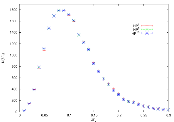
Figure 1: Typical distribution of $\delta F_{x}$, Eq. (20), on thermalized $12^{4}$, $\beta=2.35$ lattices for various $\sigma$-model ranks.

Next we have to investigate how the quality of approximation depends upon the $\sigma$-model rank $n$. We calculated the distribution of $\delta F_{x}$ for $n=1,8,15$ on several fixed thermalized SU(2) configurations ($12^{4}$ lattice at $\beta=2.35$). The corresponding typical histograms are presented on Fig. 1 and clearly show that the approximation quality does not depend at all upon the rank. Thus the naive expectation that rank could serve as an ultraviolet filter turns out to be wrong. Instead we found that the approximation quality is 10-20% for ’hot’ SU(2) gauge fields irrespectively of the concrete $\mathrm{HP}^{n}$ $\sigma$-model considered. The plausible explanation of this might be as follows: from the continuum considerations we know that the equality (17) is valid for smooth (e.g., classical) SU(2) fields only. It is commonly believed that the configurations at $\beta=2.35$ are not smooth. For this reason the approximation (19) could not be exact for any rank and its quality is mainly given by the gauge fields roughness and indeed rank independent. Note that if this reasoning is valid then the approximation quality (20) provides a quantitative measure of gauge fields smoothness. The conclusion is that it is unnecessary to consider $\mathrm{HP}^{n}$ $\sigma$-models with $n>1$ and from now on we confine ourselves to the case $n=1$.

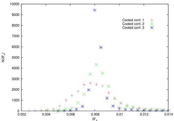
Figure 2: Distribution of $\delta F_{x}$, Eq. (20), for $\mathrm{HP}^{1}$ $\sigma$-model on three highly cooled $12^{4}$ configurations containing respectively three instantons, one anti-instanton and no instantons at all.

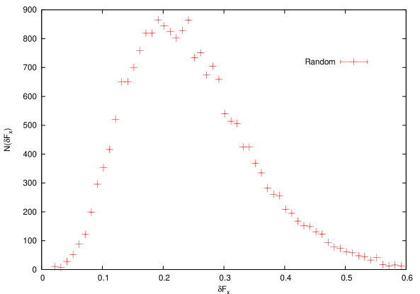
Figure 3: $\delta F_{x}$ distribution on $12^{4}$ lattice for random input gauge fields.

In view of the above discussion it is instructive to consider semiclassical and completely random input gauge fields. Using the cooling procedure (see, e.g., GarciaPerez:1998ru and references therein) we generated three highly cooled $12^{4}$ configurations containing respectively three instantons, one anti-instanton and no instantons at all. The corresponding distribution of $\delta F_{x}$ is shown on Fig. 2. It is worth to mention that the approximation quality (19) turns out be excellent, the gauge fields are reproduced with accuracy $\lesssim$ 1% in the whole lattice volume. Note that for non-trivial classical background the distribution of $\delta F_{x}$ is slightly broader then that for trivial case still reproducing the input gauge fields almost exactly. As far as the random gauge fields are concerned, the results obtained in this case (Fig. 3) support the above argumentation. Namely, the distribution of $\delta F_{x}$ values is much broader being significantly large even at $\delta F_{x}\approx 0.5$. The corresponding quality of approximation could be estimated as $\langle\delta F_{x}\rangle\approx 0.3$ and indeed is much worse then that in previous cases.

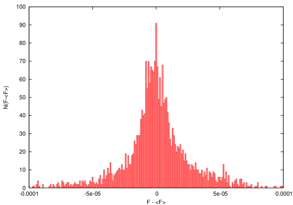
Figure 4: Distribution of the minimal values of the functional (20) (with mean value subtracted) calculated on $12^{4}$ $\beta=2.35$ thermalized lattices and averaged over 20 configurations, see text.

The last problem to be considered in this section is the problem of Gribov copies usually associated with minimization of functionals like (20). The problem lies in the fact that there might be many local minima of (20) which are relatively far apart in the configuration space of $|\,q_{x}\,\rangle$ fields. To investigate this issue we performed the following calculation. For a particular thermalized gauge configuration ($12^{4}$ lattice at $\beta=2.35$) the minimization of (20) was repeated 50 times starting every time with some random $|\,q_{x}\,\rangle$. From the deviations of found minimal values from their mean the distribution histogram was constructed and averaged over 20 input gauge configurations. In order to quantitatively address the Gribov copies problem one should compare the width of $F$ values distribution obtained this way and the precision of the functional (20) calculation which in our case could be estimated as $\approx 10^{-6}$. The distribution of the minimal values of $F$ is shown on Fig. 4 and its width turns out to be of order $\approx 10^{-5}$. The conclusion is that the Gribov copies problem is likely to be inessential in finding the $\mathrm{HP}^{1}$ $\sigma$-model for given SU(2) gauge background. However, for safety reasons we always tried 10 random initial configurations $|\,q_{x}\,\rangle$ in our minimization procedure and then selected the best minimum found.

III.2 Topological Charge Density

As we already mentioned the topological charge density in terms of the $\mathrm{HP}^{1}$ $\sigma$-model fields is given by the oriented 4-volume of spherical tetrahedron $T$ embedded into $S^{4}$. The necessity to consider 4-dimensional simplices could be deduced already from the continuum expression (15) which depends upon unit vectors $n^{A}_{(i)}$ at five infinitesimally close neighboring points marked by index $i=0,...,4$. On the lattice the vertices of the tetrahedron $T=\{n^{A}_{(i)}\}\in S^{4}$ become finitely separated and should be connected pairwise by shortest geodesics thus forming a spherical tetrahedron embedded into $S^{4}$.

To the best of our knowledge the volume of spherical four dimensional tetrahedron is unknown analytically contrary to the case of three dimensions (see, e.g., Refs. 3tetrahedron and references therein). Therefore, the only way to proceed is to invent some reasonable numerical algorithm to evaluate the 4-volume in question. Note that this is so because we are specifically interested in the topological charge density. As far as only the global topological charge is of concern, one could proceed in usual way utilizing the fact that the topological density is almost the total derivative (see, e.g., Ref. Gerrit ). Then the evaluation of the global charge reduces to the calculation of the volumes of three-dimensional spherical simplices which could be done analytically.

The most straightforward way to estimate the 4-volume of spherical simplex is to use the Monte Carlo technique, the essence of which is to pick up a random point in $S^{4}$ and to decide whether it is inside or outside the spherical tetrahedron. Due to the simplicity of $S^{4}$ geometry the last question reduces to the relatively fast calculation $5\times 5$ determinants analogously to the case of $S^{3}$ sphere considered in Stone . However, proceeding this way we definitely loose the integer valuedness of the topological charge since volume of every simplex (topological charge density) is calculated with finite accuracy. Evidently the accuracy should be small enough to recover the topological charge and simultaneously large enough to be practically reasonable. In our test runs (see below) we found that the optimal relative accuracy of the spherical tetrahedron volume estimation should be smaller then 2%.

Now we can summarize our algorithm of topological charge density calculation.

1. On input there are five unit 5-dimensional vectors $n^{A}_{(i)}$, $i=0,...,4$ sitting at five vertices of simplex ${\cal T}$ of the physical space triangulation. The vectors $n^{A}_{(i)}$ are constructed via Eq. (13) and provide the mapping of ${\cal T}$ into the spherical tetrahedron $T\in S^{4}$, the oriented volume $V(T)$ of which is to be calculated. Generically the set $n^{A}_{(i)}$ is not degenerated $\mathrm{det}_{iA}\,[n^{A}_{(i)}]\neq 0$. Note that for $|\mathrm{det}_{iA}\,[n^{A}_{(i)}]|<10^{-10}$ we equate $V(T)$ to zero.

2. In order to speed up the Monte Carlo integration we calculate the normalized mean vector $N\propto\sum_{i}n_{(i)}$ and find the 5-dimensional cone $C$ around $N$ containing all the $n_{(i)}$. Since $V(T)<V(C\cap S^{4})$ the tetrahedron volume is equated to zero if $V(C\cap S^{4})<10^{-8}$.

3. The Monte Carlo estimation of $V(T)$ begins with picking up $10^{3}$ random points uniformly distributed in $C\cap S^{4}$. If none of them falls into the interior of $T$ the tetrahedron volume is equated to zero. Otherwise we continue to generate uniformly in $C\cap S^{4}$ random points until the volume $V(T)$ is known with accuracy 2%. Finally, the topological charge density in the simplex ${\cal T}$ of physical space triangulation is given by

$$q({\cal T})=\frac{3}{8\pi^{2}}\,\mathrm{sign}\left(\mathrm{det}_{iA}\,[n^{A}_{(i)}]\right)\cdot V(T)\,,$$ (21)

where the normalization factor $8\pi^{2}/3$ is the volume of $S^{4}$. The corresponding topological charge is

$$Q_{float}=\sum\limits_{\cal T}q({\cal T})\,,$$ (22)

where we have explicitly indicated that it is not integer valued. We remark that in order exploit this procedure on usual hypercubical lattices the hypercubes should be sliced into simplices. We did this according to the prescription of Ref. Kronfeld:1986ts .

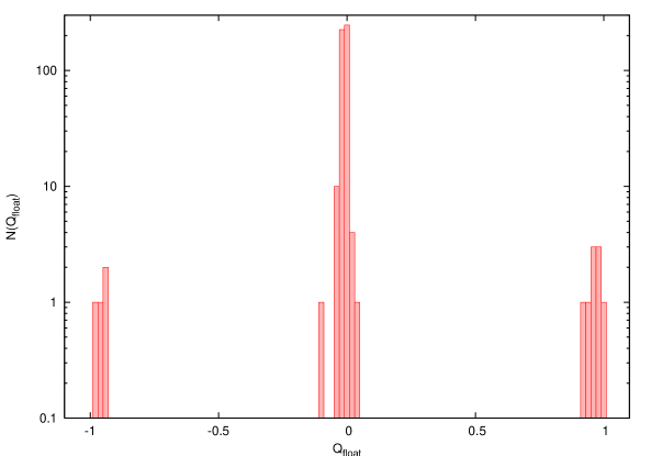
Figure 5: Distribution of the topological charge $Q_{float}$, Eq. (22), for single 5-dimensional simplex with random $\mathrm{HP}^{1}$ $\sigma$-model fields at its vertices.

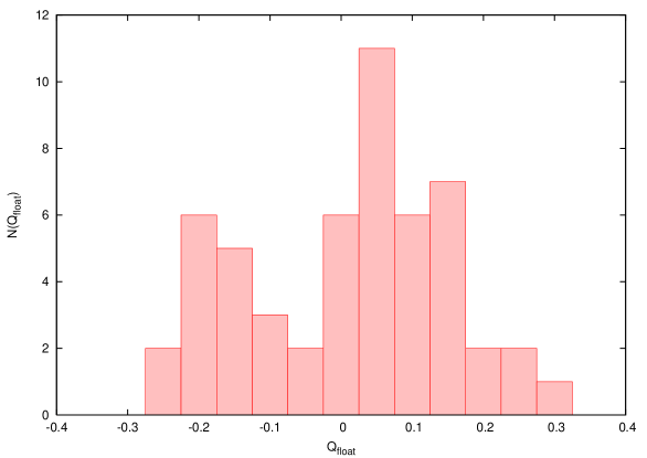
Figure 6: Distribution of $Q_{float}-Q$, Eqs. (22), (23), calculated on 55 configurations thermalized at $\beta=2.40$ on $16^{4}$ lattice.

The disadvantage of the algorithm is that the topological charge is not integer valued. However, for small enough accuracy of calculation at each simplex the problem is likely to be inessential. In order to check this we performed the following tests. First, we generated 500 sets of six random 5-dimensional unit vectors which are geometrically assigned to the vertices of 5-dimensional tetrahedron, the boundary of which consists of six 4-dimensional simplices and is $S^{4}$ topologically. Each generated set is the mapping $S^{4}\to S^{4}$ and we applied our algorithm to calculate the distribution of $Q_{float}$. The resulting histogram is presented on Fig. 5 and clearly shows that for this test the chosen accuracy is more then enough since the topological charge is sharply peaked around integer values. However, this simple test could not be completely convincing since in Eq. (22) the uncertainties coming from each simplex ${\cal T}$ are accumulating. Thus the deviation of the topological charge (22) from nearest integer increases with lattice volume $V$ and for given accuracy per each simplex the distribution of the topological charge flattens in the limit $V\to\infty$. Therefore we must ensure that for the lattices we’re going to consider and for the chosen accuracy per each simplex the distribution of $Q_{float}$ is indeed peaked around integers. Below we discuss the physically relevant results obtained on $16^{4}$ lattices at $\beta=2.4,2.475$. Since the distribution of $Q_{float}$ is technical rather then physical issue it is presented in this section. The distribution of non-integer part of the topological charge (22) calculated on $16^{4}$ lattice at $\beta=2.40$ with 55 configurations is shown on Fig. 6. As expected the histogram is much broader then that on Fig. 5, but nevertheless is still reasonably sharp with distribution width being $\approx 0.2$. We conclude therefore that for the chosen parameters and lattice volumes we could safely identify the topological charge as

$$Q=\left[\,Q_{float}\,\right]\,,$$ (23)

where $[x]$ denotes the nearest to $x$ integer number. We stress that the identification (23) is not universal and is valid only for particular range of parameters and lattice volumes. From now on the term “topological charge” will refer exclusively to the integer valued quantity $Q$.

Unfortunately, the presented algorithm turns out to be very time consuming. As a matter of fact there is no hope to use it on single processor machines. Indeed, the considered triangulation of one 4-dimensional hypercube consists of $16$ simplices and their total number becomes prohibitively large for any reasonable lattice volumes. However, it is very easy to implement the method on computer clusters since calculation of the topological charge density is done independently for each simplex.

III.2.1 Testing the Algorithm

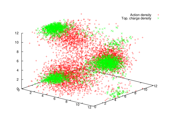
Figure 7: Time slice of the action and the topological charge densities (21) on cooled $12^{4}$ configuration containing three instantons.

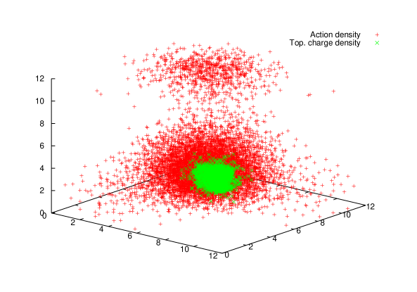
Figure 8: Time slice of the action and the topological charge densities (21) on cooled $12^{4}$ configuration containing one anti-instanton.

The approximate integer valuedness of the topological charge is not the only test which our algorithm should pass. At least we should convince ourselves that the method works in the case of (quasi)classical configurations and compare it with known topological charge constructions.

As far as the quasi-classical fields are concerned we applied our method to the same set of highly cooled $12^{4}$ configurations generated in section III.1. We have seen that the approximation quality of SU(2) gauge matrices by the corresponding $\mathrm{HP}^{1}$ $\sigma$-model fields was almost excellent (about 1%). Now we compare the local gauge action and the density of the topological charge on these configurations. It turns out that they agree just nicely as shown on Fig. 7, 8, where for a particular time slice $t=2$ the amount of red (green) points per 3-dimensional lattice cube is proportional to the action (absolute value of the topological charge) density. On the first configuration (Fig. 7) our algorithm identified three instantons with total topological charge being $Q_{float}=2.91$. On the second configuration (Fig. 8) we found one anti-instanton and the topological charge is $Q_{float}=-0.98$. Note that the regions where the topological charge density is significant are rather large, their volumes are about $3^{4}$ in lattice units.

To summarize, we are confident that our method works as expected on quasi-classical configurations. Next we would like to compare it with becoming standard nowadays overlap-based topological charge definition overlap .

III.2.2 Comparison with Overlap-Based Topological Charge

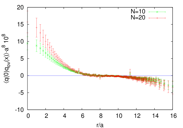
Figure 9: Correlation function (26) of the overlap- and $\mathrm{HP}^{1}$ $\sigma$-model based definitions of the topological charge density, see text.

The validity of the topological charge construction we discussed so far could only be convincing provided that we confront it with other known topological charge definitions. As far as field-theoretical DiVecchia:1981qi and geometrical Luscher ; Stone constructions are concerned, they could be applied in fact only on cooled configurations Pugh and we refuse the corresponding comparison for this reason. On the other hand, the definition overlap based on the overlap Dirac operator Neuberger:1997fp

$$q_{o}(x)=-\mathrm{tr}\,\gamma^{5}\left(1-\frac{1}{2}D_{x,x}\right)$$ (24)

is free from the above disadvantages. For reasons to be discussed in section IV.3.3 we will not consider the full trace in Eq. (24), but restrict it to $N$ lowest eigenmodes $D\psi^{(i)}=\lambda_{i}\psi^{(i)}$

$$q^{N}_{o}(x)=-\sum\limits_{i<N}(1-\frac{\lambda_{i}}{2})c^{(i)}(x)\,,$$ (25)

$$c^{(i)}(x)={\psi^{(i)}_{x}}^{\dagger}\gamma^{5}\psi^{(i)}_{x}\,.$$

The quantity $q^{N}_{o}$ is known as the effective topological density Horvath-qq .

In order to make a quantitative comparison of the definitions (21) and (25) we measured the correlation function Cundy:2002hv

$$C(x)=\langle q(0)\,q^{N}_{o}(x)\rangle$$ (26)

on 18 statistically independent $16^{4}$ configurations thermalized at $\beta=2.475$. The results corresponding to $N=10$ and $N=20$ lowest eigenmodes taken into account are presented on Fig. 9. It is apparent that both definitions are indeed compatible with each other and determine the topological density consistently. Moreover, the graph shown on Fig. 9 is very similar to the corresponding one given in Ref. Cundy:2002hv , where the overlap-based and field-theoretical constructions were compared.

To summarize, we found clear evidences that our construction of the topological charge density is locally correlated with overlap-based definition. This provides a stringent test of our approach and allows us move directly to the investigation of the SU(2) gauge fields topology.

IV Topology of SU(2) Gauge Fields

$\beta$ $a$,fm $L_{s}$ $L_{t}$ $V^{phys},\mathrm{fm}^{4}$ $N_{conf}$ 2.40 0.1193(9) 16 16 13.3(4) 55 2.475 0.0913(6) 16 16 4.6(1) 18

Table 1: Simulation parameters.

In this section we discuss the measurements performed with $\mathrm{HP}^{1}$ $\sigma$-model construction of the topological charge in pure SU(2) lattice gauge theory. In section IV.1 the dynamics of embedded $\mathrm{HP}^{1}$ $\sigma$-model is briefly considered. Then in section IV.2 we present our results concerning global topological charge distribution and topological susceptibility. Section IV.3 is devoted to the detailed investigation of the topological charge density bulk distribution and the corresponding correlation function. Our calculations were performed on two sets (Table 1) of statistically independent SU(2) gauge configurations generated with standard Wilson action. The lattice spacing values quoted in the Table 1 are taken from Ref. Lucini:2001ej and fixed by the physical value of SU(2) string tension $\sqrt{\sigma}=440~{}\mathrm{MeV}$. As we noted already the method we employed for topological charge density calculation is very time consuming and this explains the relatively small number of configurations we were able to analyze.

IV.1 Dynamics of the Embedded $\mathrm{HP}^{1}$ $\sigma$-model

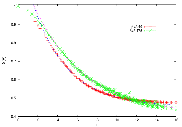
Figure 10: The correlation function (27) in the embedded $\mathrm{HP}^{1}$ $\sigma$-model. Lines correspond to the best fitting curves (28).

Given that in our approach the calculation of the topological properties of SU(2) gauge fields requires the construction of $\mathrm{HP}^{1}$ $\sigma$-model it is natural to consider the dynamics of the embedded scalar fields. The basic correlation function in the $\mathrm{HP}^{n}$ $\sigma$-models is given by

$$G(x)~{}=~{}\langle\mathrm{Sc}\,\mathrm{tr}\,[\,P(0)P(x)\,]\rangle\,,$$ (27)

where $P_{ik}$ are the quaternionic valued projector matrices (11). Note that we didn’t subtracted the disconnected part of $G(x)$. The physical meaning of the correlation function (27) could well be illustrated for $\mathrm{HP}^{1}$ $\sigma$-model where it reduces up to irrelevant constant contributions to $G(x)=\langle\sum_{A}n^{A}_{0}n^{A}_{x}\rangle$. On general grounds one expects that the embedded $\mathrm{HP}^{n}$ $\sigma$-models could be in two different phases distinguished by $G(x)$. Namely, the correlator (27) falls off exponentially at large $|x|$ in massive (disordered) phase and only with some inverse power of $|x|$ in the massless (ordered) phase. Taking into account the quality of the approximation (19) discussed in section III.1 one could argue that the confinement (deconfinement) phase of gluodynamics might be reflected by the disordered (ordered) phase in the corresponding $\sigma$-models. At present it is too early to discuss this conjecture quantitatively, but our preliminary studies indicate that it is indeed reasonable. The data we have right now refer to the confinement phase exclusively where we expect the exponential behavior of the correlator (27)

$$G(|x|\to\infty)~{}\approx~{}C_{0}\,\,e^{-m|x|}~{}+~{}C_{1}\,.$$ (28)

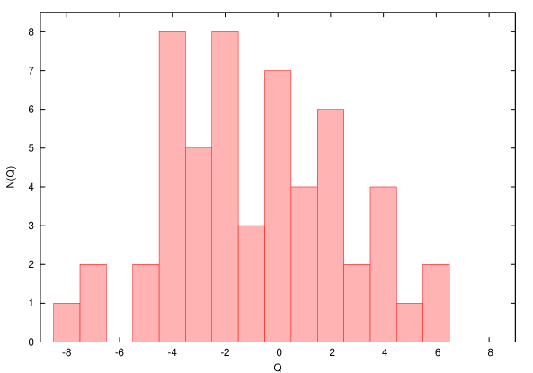
Figure 11: Topological charge distribution calculated on $\beta=2.40$ configurations.

The results of our measurements of the correlation function (27) are presented on Fig. 10 (left). To investigate the large distance behavior of $G(x)$ we fitted the data to Eq. (28) in various ranges of $R=|x|$. The fits turn out to be rather stable, the best fitting curves are shown on Fig. 10 by dashed lines. The results of various fits strongly suggest that the parameter $m$ entering Eq. (28) is nothing but the SU(2) string tension

$$m~{}=~{}a\,\sqrt{\sigma}\,,$$ (29)

being equal to $m_{\beta=2.40}=0.28(2)$ and $m_{\beta=2.475}=0.19(1)$ at the $\beta$ values considered. In fact, Eq. (29) indirectly supports the above made conjecture on the phase diagram of the embedded $\mathrm{HP}^{1}$ $\sigma$-model.

IV.2 Topological Charge

We should mention that the limited set of configuration we have in our disposal prevents us from studying the topological charge distribution and related quantities with sufficient accuracy. Nevertheless our results allow to draw some preliminary conclusions about the method we presented. There are two basic quantities to be discussed here, the topological charge (23) distribution and the topological susceptibility $\chi=\langle Q^{2}\rangle/V$.

The distribution of the topological charge for $\beta=2.40$ is shown on Fig. 11. Although the width of the histogram is roughly what is expected at this $\beta$ value, the shape of the distribution seems to indicate the lack of statistics. In particular, it is hardly possible to fit it with Gaussian profile. Moreover, the noticeable asymmetry in odd/even $Q$ values should also be mentioned, which probably hints on some subtle issues in our topological charge definition. Anyhow, the evident lack of statistics prohibits us to make solid conclusions at the moment. For the same reason we do not present the analogous histogram at $\beta=2.475$ since the statistics in this case is even worse.

As far as the $\langle Q^{2}\rangle$ and the topological susceptibility are concerned, their values turn out to be

$$\begin{array}[]{c|c|c}\beta&\,\,\,\,\langle Q^{2}\rangle&\,\,\,\,\chi\\ \hline\cr 2.40&\,\,\,\,10.8\pm 1.8&\,\,\,\,(190(10)\mathrm{~{}MeV})^{4}\\ \hline\cr 2.475&\,\,\,\,3.9\pm 1.0&\,\,\,\,(192(12)\mathrm{~{}MeV})^{4}\end{array}$$ (30)

which indicate a perfect scaling and are fairly consistent with data of Ref. Lucini:2001ej .

To summarize, at present our calculation of the global topological charge is plagued by the lack of statistics and should be improved to quantify our method. Nevertheless, qualitatively our results are in agreement with the literature and don’t show any pathology in the approach we have developed.

IV.3 Topological Charge Density

The topological charge density $q(x)$ is defined by Eq. (21) and provides quantitative characterization the topological charge bulk distribution. As a first qualitative illustration we present visualization of $q(x)$ in particular time-slice of four dimensional lattice. It turns out that the corresponding pictures at various slices look very similar. The typical distribution of $q(x)$ is shown on Fig. 12 (data is taken on $16^{4}$, $\beta=2.40$ lattices). Here the density of points is proportional to the absolute value $|q(x)|$ while red (green) points mark the regions of positive (negative) topological charge density. Note that the empty areas correspond to indeed either vanishing or at least utterly small $|q(x)|$.

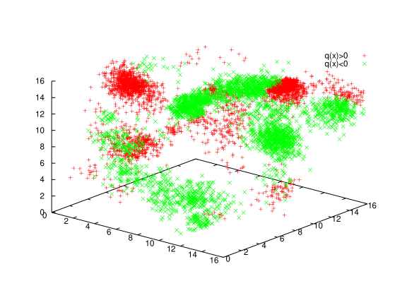
Figure 12: Visualization of the topological charge density distribution in a particular time slice of $16^{4}$, $\beta=2.40$ thermalized configuration.

Several qualitative comments are now in order. It is apparent and remarkable that the topological charge density is distributed in localized regions which roughly look like four dimensional balls. As a matter of fact this regions are almost spherically symmetric resembling instantons from the first sight. We are in hustle to add however that we don’t claim that these regions are indeed the instantons (see below). In either case the lumpy structure of the topological charge density is present in all configurations we have and could be taken as firmly established. Note that this result is not new, the lumpy distribution of the topological charge in “hot” (not cooled, smoothed or smeared in any way) vacuum configurations was observed already in Refs. Gattringer ; DeGrand ; Hip ; Horvath:2002gk . However, we found the lumps completely independently using newly developed method which not only confirms their existence but also provides new opportunities to investigate the structure of the lumps. The second point is that the lumps ${\cal L}_{i}$ in $q(x)$ distribution are significantly dilute, their total number in every time slice could be estimated as $\lesssim 10$, the corresponding lumps density being $D_{\cal L}\approx 3\cdot 10^{-3}$ in lattice units which translates to $D_{\cal L}\approx 10\mathrm{~{}fm}^{-4}$ for $\beta=2.40$. At the same time it is apparent that the lumps are clearly separated from each other and their characteristic size is of order $\rho_{\cal L}\approx(1\div 2)a\approx 0.12\div 0.24\mathrm{~{}fm}$.

The reminder of this section is organized as follows. In section IV.3.1 we describe in details our approach aimed to investigate the lumpy structure described above. In particular, we argue that in order to quantitatively define the notion of lumps it is mandatory to introduce the physically motivated cutoff $\Lambda_{q}$ on $|q(x)|$ values and to ensure that final results are cutoff independent in reasonably large range of $\Lambda_{q}$. In section IV.3.2 we explore the limit $\Lambda_{q}\to 0$ which seems to be unphysical for us, but in which we find that the topological charge organizes into some global structures reminiscent to ones discovered recently Horvath-structures . Then in section IV.3.3 we present our results for the topological charge density correlation function and discuss some related issues. Until section IV.3.4 we consider only the data collected on $16^{4}$, $\beta=2.40$ lattices, while in section IV.3.4 the comparison is made with the results obtained at $\beta=2.475$.

IV.3.1 Lumps in $q(x)$ Distribution

In order to investigate quantitatively the nature of the lumps ${\cal L}_{i}$ in the topological charge density we have to define first an algorithm to identify the lumps. The natural procedure is to apply some cutoff $\Lambda_{q}$ to the topological density and to treat the small values $|q(x)|<\Lambda_{q}$ as identical zero. It is expected that for reasonably wide range of $\Lambda_{q}$ the lumps ${\cal L}_{i}$ would look like an isolated 4-dimensional regions of sign-coherent topological charge. It is clear that the number of lumps and other their characteristics depend upon the cutoff $\Lambda_{q}$. We expect that the universal physical properties of the lumps in $q(x)$ distribution should be independent or depend only mildly on $\Lambda_{q}$ (in the second case the bias introduced by $\Lambda_{q}$ dependence is to be included into systematic errors).

Notice the following two extreme cases. Evidently, for large $\Lambda_{q}$ there would be no lumps at all and hence the maximal cutoff coincides by order of magnitude with the maximal value of $|q(x)|$. On the other hand for $\Lambda_{q}=0$ one expects to find a large amount of very small lumps consisting of just one lattice point. There are at least two reasons to justify this assumption. First, this is because we constructed the $\mathrm{HP}^{1}$ $\sigma$-model starting from “hot” thermalized gauge configurations and $|\,q\,\rangle$ fields reflect partially the ultraviolet noise present in the original gauge potentials. Therefore, away from the lumps the topological density is expected to fluctuate widely around zero while being almost vanishing in magnitude. Secondly, it is quite evident that it makes no sense to assign any physical meaning to utterly small $|q(x)|$. The physically meaningful minimal $\Lambda_{q}$ value could be estimated by order of magnitude as the ratio of typical topological charge and the lattice volume, which for our lattices is $\approx 10^{-5}$. We conclude therefore that the extremely small cutoff $\Lambda_{q}\cdot a^{4}<10^{-5}$ could not have any physical significance and the universal properties of the topological density bulk distribution (universality window) should be looked for in $\Lambda_{q}\cdot a^{4}>10^{-5}$ region.

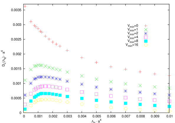
Figure 13: Dependence of the lumps density $D_{\cal L}$ upon the cutoff $\Lambda_{q}$ for various values of $V_{min}$, Eq. (31).

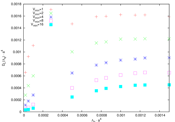
Figure 14: $D_{\cal L}(\Lambda_{q})$ dependence in the range $10^{-5}<\Lambda_{q}\cdot a^{4}<1.5\cdot 10^{-3}$ for various $V_{min}$, Eq. (31).

Let us consider first the dependence of the total lumps density $D_{\cal L}$ upon the cutoff $\Lambda_{q}$, which is shown by the upper curve on Fig. 13. As expected from the discussion above $D_{\cal L}$ is monotonically decreasing function of $\Lambda_{q}$ and diverges in the limit $\Lambda_{q}\to 0$. However, the dependence $D_{\cal L}(\Lambda_{q})$ becomes less trivial if we consider only lumps satisfying

$$V({\cal L}_{i})~{}>~{}V_{min}\gtrsim 1\,,$$ (31)

where $V({\cal L}_{i})$ is the total number of sites constituting the lump ${\cal L}_{i}$ and $V_{min}$ is taken to be of order few units. In fact, the constraint (31) is quite natural since for $V_{min}=1$ it cuts only smallest fraction of UV-scale lumps. It is remarkable that already from $V_{min}=1$ onward the shape of $D_{\cal L}(\Lambda_{q})$ dependence is universal, the only thing which distinguishes the curves at various $V_{min}$ is the scale of the density $D_{\cal L}(\Lambda_{q})$. Note that the behavior of $D_{\cal L}$ in the limit $\Lambda_{q}\to 0$ is changing qualitatively once the volume cutoff is imposed. As is apparent from Fig. 14, for any $V_{min}>0$ we have

$$\lim\limits_{\Lambda_{q}\to 0}\left.D_{\cal L}\,\right|_{V_{min}>0}=const<\infty$$ (32)

and this is discussed in the next section. The maximum of the function $D_{\cal L}(\Lambda_{q})$ at $V_{min}>0$ and its rather mild dependence on $\Lambda_{q}$ for

$$\Lambda_{q}>10^{-3}\cdot a^{-4}=(290\mathrm{~{}MeV})^{4}$$ (33)

suggests that $\Lambda_{q}$ universality window starts from this value.

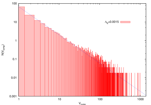
Figure 15: Distribution of lumps volumes, Eq. (34), for $\Lambda_{q}\cdot a^{4}=1.5\cdot 10^{-3}$ calculated on $16^{4}$, $\beta=2.40$ lattices and normalized by the number of configurations. Solid line is the fit to Eq. (35).

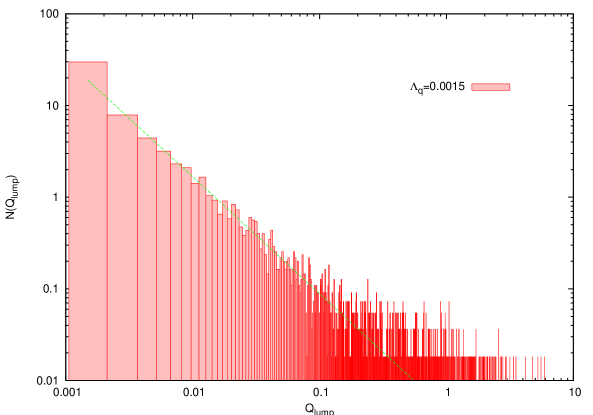
Figure 16: Lumps charge, Eq. (34), distribution for $\Lambda_{q}\cdot a^{4}=1.5\cdot 10^{-3}$ calculated on $16^{4}$, $\beta=2.40$ lattices and normalized by the number of configurations. Solid line is the fit to Eq. (35).

Let us now consider the volumes and the topological charges of the lumps ${\cal L}_{i}$

$$V({\cal L}_{i})=\sum\limits_{x\in{\cal L}_{i}}1\,,\qquad Q({\cal L}_{i})=\sum\limits_{x\in{\cal L}_{i}}q(x)\,,$$ (34)

identified for given value of $\Lambda_{q}$. The distributions of $V({\cal L}_{i})$ and $Q({\cal L}_{i})$ for $\Lambda_{q}\cdot a^{4}=1.5\cdot 10^{-3}$ calculated on $16^{4}$, $\beta=2.40$ lattices and normalized by the number of configurations are shown on Fig. 15 and Fig. 16 respectively. A few points are worth to be mentioned here. First, we see that both volume and charge distributions are well described by power laws

$$N[V({\cal L}_{i})]=c_{V}\cdot[V({\cal L}_{i})]^{-\alpha_{V}}\,,$$ (35)

$$N[Q({\cal L}_{i})]=c_{Q}\cdot[Q({\cal L}_{i})]^{-\alpha_{Q}}\,,$$

for not exceptionally large $V({\cal L}_{i})$ and $Q({\cal L}_{i})$. On the other hand the appearance of extremely large lumps with volumes $V({\cal L}_{i})\gtrsim 100\cdot a^{4}$ and charges $Q({\cal L}_{i})\gtrsim 1$ is cutoff dependent (see below). Therefore, let us concentrate on the behavior (35) valid for moderate $V({\cal L}_{i})$ and $Q({\cal L}_{i})$. It turns out that both histograms in the almost entire ranges of volumes and charges are well described by Eq. (35) and the fitted values of power exponents are given by

$$\left.\alpha_{V}\right|_{\Lambda_{q}\cdot a^{4}=0.0015} = 1.52(8)\,,$$ (36)

$$\left.\alpha_{Q}\right|_{\Lambda_{q}\cdot a^{4}=0.0015} = 1.32(20)\,,$$

where a conservative error estimates are quoted. Apparently both power exponents are compatible with each other and it is tempting to conclude that for $\Lambda_{q}\cdot a^{4}=1.5\cdot 10^{-3}$ they are equal to

$$\alpha_{V}~{}=~{}\alpha_{Q}~{}=~{}3/2\,.$$ (37)

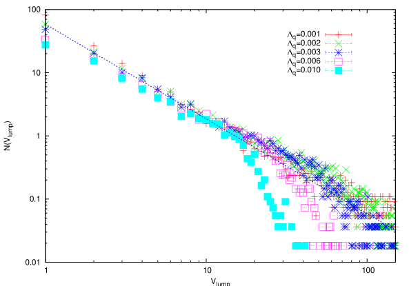
Figure 17: Lumps volume distribution for various $\Lambda_{q}$ given in lattice units. Solid line is the fit (35) with $\alpha_{V}=3/2$.

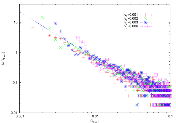
Figure 18: Distribution of lumps charges for different $\Lambda_{q}$ given in lattice units. Solid line is the fit (35) with $\alpha_{Q}=3/2$.

Clearly, we should check this conjecture at very least by investigating the dependence of power exponents upon the cutoff $\Lambda_{q}$. The corresponding histograms are presented on Fig. 17 and Fig. 18 where we have collected the distributions of $V({\cal L}_{i})$ and $Q({\cal L}_{i})$ obtained for various $\Lambda_{q}$ on $16^{4}$, $\beta=2.40$ configurations. The solid lines on the figures represent the one-parameter fits to Eq. (35) in which we have fixed $\alpha_{V}$ and $\alpha_{Q}$ according to Eq. (37). It is remarkable that the volumes of the lumps are distributed well within numerical uncertainties in agreement with (35) at all values of the cutoff. The only deviation from (35) is seen at large $\Lambda_{q}$, $V({\cal L}_{i})$ and could be easily understood. Indeed, for very large $\Lambda_{q}$ we will not find any lumps at all and with diminishing cutoff we start seeing lumps from some finite volume only. This could explain the apparent drop in the $V({\cal L}_{i})$ distribution for $\Lambda_{q}\cdot a^{4}$ equal to $6\cdot 10^{-3}$ and $10^{-2}$. Essentially the same arguments apply to the $Q({\cal L}_{i})$ histograms which show a slight deviation from (35) for large $\Lambda_{q}$ and small $Q({\cal L}_{i})$. Thus the have found an universal (cutoff independent) behavior (35), (37) of the lumps volume and charge distributions for $\Lambda_{q}\cdot a^{4}>10^{-3}$. In the next section we show that for smaller $\Lambda_{q}$ this universality does not hold. Therefore we have clear evidences that the lower bound of the cutoff universality window is indeed given by (33).

Let us make a few comments concerning the distribution (35), (37). The simplest possible picture behind the lumpy structure of the topological density is that $q(x)$ is non-vanishing only within the four dimensional balls of radius $\rho$. It is reminiscent to the well known instantonic picture of the vacuum and in this case the power law (35), (37) translates into

$$N[\rho]\,d\rho~{}\sim~{}\frac{d\rho}{\rho^{3}}\,,$$ (38)

which is precisely the instantons distribution elaborated in Ref. Diakonov . While the microscopic view of the lumps as four dimensional balls of sign-coherent topological charge looks quite natural, it is in fact incompatible with instantons. Indeed, Eqs. (35), (37) imply that the lumps are objects with fractional and arbitrary small charge. As far as the large lumps with $Q({\cal L}_{i})\approx 1$ are concerned we discuss them in the next section, but right now it is enough to mention that their number is negligible compared to the total number of lumps. The conclusion is that the majority of the lumps are not the instantons.

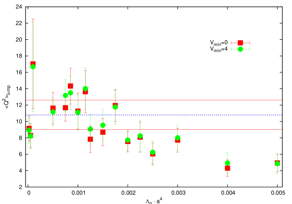
Figure 19: Lumps limited squared topological charge $\langle Q^{2}\rangle_{lump}$ versus cutoff $\Lambda_{q}$. Lines represent $\langle Q^{2}\rangle$, Eq. (30), and the corresponding error bounds.

The question of primary importance is whether the total topological charge is dominated by the lumps. The relevant quantity is the lumps limited topological susceptibility which is essentially $\langle Q^{2}\rangle$ measured on the lumps only. Note that this quantity naturally bounds the physically acceptable cutoff from above. Indeed, for vanishing cutoff the lumps limited average $\langle Q^{2}\rangle_{lump}$ coincides with the full one, $\langle Q^{2}\rangle_{lump}=\langle Q^{2}\rangle$, while at very large $\Lambda_{q}$ we would have $\langle Q^{2}\rangle_{lump}=0$. The characteristic cutoff at which the topological susceptibility drops down is definitely the upper bound on physical $\Lambda_{q}$ and a priori could be on the either side of the value quoted in (33). The lumps would be clearly unphysical if $\Lambda_{q}$ range happens to be empty.

We have measured the lumps limited squared topological charge $\langle Q^{2}\rangle_{lump}$ on $16^{4}$ $\beta=2.40$ configurations, the result is presented on Fig. 19. Note that we also checked the dependence of $\langle Q^{2}\rangle_{lump}$ on the volume cutoff (31) which turns out to be trivial as is clear from the figure. Indeed, the data points with volume cut $V_{min}=4$ imposed are falling on the top of the data with no volume cut at all. It is apparent that the topological susceptibility is indeed lumps dominated provided that

$$\Lambda_{q}<2\cdot 10^{-3}\,a^{-4}=(350\mathrm{~{}MeV})^{4}\,.$$ (39)

Note that the universality window (33), (39) appears to be rather small. However, this does not appear completely unexpected. Indeed, our original intent was to find a plateau in the cutoff dependence of various quantities characterizing the lumps, at which their first $\Lambda_{q}$ derivative vanishes. In particular, the universality window (33), (39) could be estimated rather precisely by noting that the maximum of the lumps density $D_{\cal L}(\Lambda_{q})$ at any $V_{min}\gtrsim 1$ is located roughly at

$$\Lambda^{*}_{q}~{}=~{}(1\div 1.5)\,10^{-3}\cdot a^{-4}~{}=~{}(314(16)\mathrm{~{}MeV})^{4}\,,$$ (40)

which almost coincides with the universality window range.

Finally, let us note that the question of dislocations, which a priori could be crucial for our investigation, is likely to be irrelevant in fact. For general arguments, which we could just verbosely repeat here and which show that dislocations are not essential in our case, the reader is referred to Ref. Horvath:2002gk . We could only add that the dislocation filtering (as well as partial filtering of the UV noise) is built into our approach. Moreover, we don’t see any sign of dislocations in the topological susceptibility which seems to be perfectly scaling and is in a good agreement with its accepted value. Following Ref. Horvath:2002gk we stress that the notion of dislocation is indispensable from both the gauge action and the topological charge operator. Therefore due to the specific properties of our topological charge construction we expect that the issue of dislocations inherent to Wilson gauge action is not applicable in our case.

IV.3.2 Exploring the Limit $\Lambda_{q}\to 0$

In this section we explore the limit of vanishing cutoff imposed on the topological charge density. Although it is not clear for us what is the physical relevance of the limit $\Lambda_{q}\to 0$ it nevertheless seems to be interesting to consider in connection with recent observation of low-dimensional global structures in the topological charge density distribution Horvath-structures . Essentially, these global structures are defined as topological charge sign-coherent regions and thus are similar to the lumps we’re investigating.

In fact, the non-trivial features of the $\Lambda_{q}\to 0$ limit could be seen already on Fig. 14 from which it follows that once the mildest $V_{min}=1$ volume cut is imposed the density of lumps rapidly diminishes with decreasing $\Lambda_{q}$ provided that $\Lambda_{q}\cdot a^{4}\lesssim 10^{-3}$. The dependence $D_{\cal L}(\Lambda_{q})$ in the range (see Fig. 14)

$$\Lambda_{q}\,\in\, [\,2\cdot 10^{-5}\cdot a^{-4}\,;\,10^{-3}\cdot a^{-4}\,] =$$ (41)

$$= [\,(110\mathrm{~{}MeV})^{4}\,;\,(290\mathrm{~{}MeV})^{4}\,]$$

makes it apparent that $D_{\cal L}(0)$ is very small if not non-vanishing. However, the total number of lumps (no volume cut imposed) is divergent, hence the dominant contribution at small $\Lambda_{q}$ comes from lumps consisting of just one point. Then the question is whether we have any other contributions to $D_{\cal L}$ or everything is exhausted by one-point lumps.

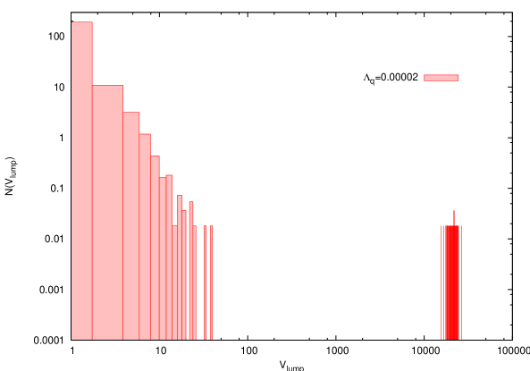
Figure 20: Lumps volume distribution for fixed cutoff $\Lambda_{q}\cdot a^{4}=2\cdot 10^{-5}$.

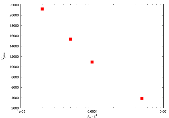
Figure 21: Volumes of percolating lumps at various $\Lambda_{q}$. Note that percolating lumps disappear at $\Lambda_{q}\cdot a^{4}\approx 7\cdot 10^{-4}$.

To investigate this issue we considered the lumps volume distribution at $\Lambda_{q}\cdot a^{4}=2\cdot 10^{-5}$ and it turns out (see Fig. 20) that it is qualitatively distinct from the case of moderate cutoff. First, we clearly see that the histogram separates into two disconnected pieces corresponding to small and extremely large (percolating) lumps. As far as the percolating lumps are concerned we didn’t investigated their properties in details for reasons to be explained shortly. We only mention that there are almost always only two percolating lumps on our configurations carrying an extremely large and opposite topological charge. Qualitatively our results are in accord with that of Refs. Horvath-structures , where the analogous percolating global structures were found. If we now turn to the consideration of small lumps distribution, it also follows sharply the law (35). However, the power exponent is drastically changing

$$\left.\alpha_{V}\right|_{\Lambda_{q}\cdot a^{4}=2\cdot 10^{-5}}=2.9(1)\,.$$ (42)

Next we compare the lumps volume distributions at various $\Lambda_{q}$ from the range (41). The first observation is that the volume of the percolating lumps strongly depends upon the cutoff imposed as is shown on Fig. 21. Moreover, the percolating lumps are present only for $\Lambda_{q}\cdot a^{4}\lesssim 7\cdot 10^{-4}$ and disappear at larger values of the cutoff. At the same time the power exponent $\alpha_{V}$ is also not universal as is clear from Fig. 22 where we have plotted the distribution of lumps with small volumes. We have also measured the function $\alpha_{V}(\Lambda_{q})$ and it is presented on Fig. 23. The power exponent $\alpha_{V}$ becomes cutoff independent only for $\Lambda_{q}\cdot a^{4}>10^{-3}$ thus justifying the choice (33), (39) made earlier for the physical range of the cutoff values.

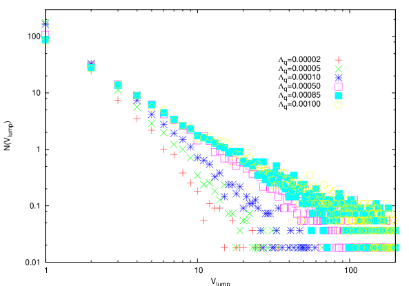
Figure 22: Distribution of the small volume lumps at various $\Lambda_{q}$. Note that it still follows the power law (35).

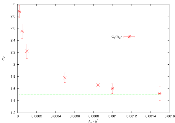
Figure 23: The power exponent $\alpha_{V}$, Eq. (35), as function of $\Lambda_{q}$ in the range (41). Line represents the conjectured universal value (37).

To summarize, it seems crucial to ensure the universality of the lumps distribution (and thus the very definition of the lumps) with respect to the a priori arbitrary choice of the cutoff on the topological charge density. Once the universality is ensured the lumps distribution follows sharply the cutoff independent power law (35) with rather remarkable value of the power exponents $\alpha_{V}\approx\alpha_{Q}\approx 3/2$. To the contrary at small $\Lambda_{q}$ we found very peculiar lumps structure. Namely the number of small lumps obeys the same power law (35) but with much large power exponent which seems to be divergent in the limit $\Lambda_{q}\to 0$. At the same time a few (typically two) percolating lumps appear which are reminiscent to the global topological structures discovered recently Horvath-structures . However, it is unclear for us what is the physical significance of the results obtained at very small $\Lambda_{q}$ since the lumps properties are strongly cutoff dependent in this limit.

IV.3.3 Topological Density Correlation Function

In this section we present our results for the topological charge density correlation function $\langle q(0)q(x)\rangle\equiv\langle qq\rangle$ obtained on our $16^{4}$, $\beta=2.40$ configurations. However, let us clarify first our view on some theoretical points concerning this correlator which were much elaborated in the recent studies Horvath-qq .

It has long been known (see Ref. Seiler:2001je and references therein) that the correlation function $\langle qq\rangle$ can not be positive at non-zero physical distances. Confronted with the positivity of the topological susceptibility $\chi=\langle Q^{2}\rangle/V=\int\langle qq\rangle$ this implies a peculiar structure of $\langle qq\rangle$ correlation function, which is to be negative for $x\neq 0$, while containing non-integrable singularity (contact term) at the origin such that the susceptibility remains positive (in the context of $\mathrm{CP}^{n}$ models this issue is also discussed in Ref. Vicari:1999xx ). In fact the negativity of $\langle qq\rangle$ correlator motivated the recent discovery of the global topological structures Horvath-structures since it implies that the topological charge could not be concentrated in four-dimensional regions of finite physical size. However, we do think that the contact term in $\langle qq\rangle$ correlator is the clear sign of the perturbation theory to which the susceptibility is believed to be unrelated.

To sort out the problem consider the instanton liquid model where the identification of perturbative and non-perturbative contributions is intuitively clean. At least at small non-zero distances we have $\langle qq\rangle_{pert}\sim-1/|x|^{8}$, while $\langle qq\rangle_{non-pert}$ is positive at small $x$ and rapidly drops down at distances comparable with the characteristic instanton size (it could even become negative at larger $x$ if the instantons interaction is significant). If we suppose that the perturbative and non-perturbative parts do not mix then the negativity requirement could be fulfilled at least in principle. The outcome is that the perturbation theory could overwhelm the non-perturbative part and reproduce qualitatively the behavior of $\langle qq\rangle$ outlined above still giving vanishing contribution to the susceptibility. Then the actual question is how do we understand the topological charge density operator. The negativity requirement could hold for perturbation theory sensitive (thus presumably local) definitions of $q(x)$ and does not apply to non-perturbative ones. Thus the problem we’re discussing is essentially the same long standing problem of perturbative and non-perturbative physics separation, which seems to have no unambiguous solution (see, e.g., Ref. Zakharov:2003vd for recent discussion).

A particular illustration of the above reasoning is provided by the overlap-based construction of the topological charge overlap . It is remarkable that once only a few lowest modes of the Dirac operator are considered the topological charge density distribution has lumpy structure DeGrand ; Hip ; Horvath:2002gk while the $\langle qq\rangle$ correlation function stays non-negative at all distances. However, the inclusion of higher Dirac modes into the $q(x)$ definition results in the appearance of some global “sheets” Horvath-structures percolating through all the lattice volume and carrying extremely large topological charge. Simultaneously with increasing number of modes the $\langle qq\rangle$ correlation function becomes negative and develops the positive singularity at the origin Horvath-qq . The interpretation might be that the more modes are included the more local the definition of topological density is and hence $q(x)$ becomes more sensitive to the perturbation theory. Essentially for this reason we considered the effective topological density (25) in section III.2.2, where the overlap-based definition was compared with our construction.

It is remarkable that we also see qualitatively the same behavior with our definition of the topological charge density. The border between perturbative and non-perturbative regions is provided in our case by the universality window with respect to $\Lambda_{q}$. We have seen that the lumpy structure gradually changes with diminishing $\Lambda_{q}$ and becomes consisting of a few percolating lumps plus the divergent number of lumps having UV-scale volume. However, we stress that not only the window (33), (39) provides the separation of perturbative and non-perturbative physics. Some degree of non-locality is built into our approach from very beginning and in the spirit of the above discussion one could say that our definition of the topological density is non-perturbative by construction to which the negativity requirement does not apply. Thus we expect that the $\langle qq\rangle$ correlation function in our case should behave roughly exponentially

$$\langle qq\rangle~{}\sim~{}\exp\{\,-|x|/\rho_{\cal L}\,\}$$ (43)

with correlation length $\rho_{\cal L}$ corresponding to the characteristic lump size.

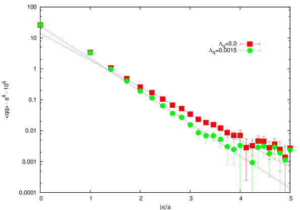
Figure 24: The topological charge density correlation function measured on $16^{4}$, $\beta=2.40$ lattices for $\Lambda_{q}\cdot a^{4}=0$ and $1.5\cdot 10^{-3}$. Lines represent the best fits (43).

The result of our measurements of the $\langle qq\rangle$ correlator on $16^{4}$, $\beta=2.40$ configurations is presented on Fig. 24. It should be noted that within the numerical errors $\langle qq\rangle$ is nowhere becoming negative and is compatible with zero from $|x|=6\cdot a$ onward. Therefore we plotted the $\langle qq\rangle$ correlator only in the range $|x|/a\in[0;5]$ where data closely follows Eq. (43). In turn, the fitted value of the characteristic lump size is given by

$$\left.\rho_{\cal L}\right|_{\Lambda_{q}=0}~{}=~{}0.50(2)\cdot a~{}=~{}0.060(3)\mathrm{~{}fm}\,,$$ (44)

where we have explicitly indicated that the data was taken without any cutoff imposed. As far as the dependence upon the cuts (33), (39) and (31) is concerned, it turns out that the $\langle qq\rangle$ correlator is independent on $V_{min}$ at non-zero separations provided that $V_{min}$ is of order unity. Indeed, the dominant contribution to $\langle qq\rangle$ comes from the extended regions of sign-coherent topological charge while the contribution of small lumps $V({\cal L}_{i})\approx 1$ averages to zero for $x\neq 0$. Note that the apparent deviation of $\langle qq\rangle$ from (43) at $|x|/a=0,1$ is due to the abundance of small lumps and practically disappears once the cut $V_{min}\approx 1$ is applied. The dependence upon $\Lambda_{q}$ could also be qualitatively established since for increasing cutoff the size of the lump contributing significantly to $\langle qq\rangle$ diminishes. In fact, $\rho_{\cal L}$ depends linearly on $\Lambda_{q}$ and for $\Lambda_{q}\cdot a^{4}=1.5\cdot 10^{-3}$ it is given by

$$\left.\rho_{\cal L}\right|_{\Lambda_{q}\cdot a^{4}=1.5\cdot 10^{-3}}~{}=~{}0.41(2)\cdot a~{}=~{}0.049(2)\mathrm{~{}fm}\,.$$ (45)

To summarize, the topological charge correlation function $\langle qq\rangle$ respects the above investigated lumpy structure of the topological charge bulk distribution. Namely, it falls exponentially with distance, the corresponding characteristic size of the lumps is given by (44) and decreases if the non-zero cutoff $\Lambda_{q}$ is applied, Eq. (45). The quoted $\rho_{\cal L}$ values are in qualitative agreement with lumps volume distribution we investigated previously, namely, it is rather small in lattice units respecting the ultraviolet divergence present in (35), (37).

IV.3.4 Scaling Check

In this section we confront the data obtained at $\beta=2.40$ and $\beta=2.475$ in order to check the scaling properties of the quantities introduced earlier. First, consider the physical range of the cutoff $\Lambda_{q}$ which could be characterized by $\Lambda^{*}_{q}$, Eq. (40). Performing the analogous calculations for $\beta=2.475$ we found that

$$\Lambda^{*}_{q}=(4\div 8)\cdot 10^{-4}\cdot a^{-4}=(340(28)\mathrm{~{}MeV})^{4}\,,$$ (46)

which is consistent with its value at $\beta=2.40$. Thus the cutoff introduced to define the lumps appears to be physical quantity with continuum value around $(300\div 350\mathrm{~{}MeV})^{4}$. Note that the range of $\Lambda_{q}$ where $\partial_{\Lambda_{q}}D_{\cal L}$ approximately vanishes is notably wider at $\beta=2.475$ then is was at $\beta=2.40$.

As far as the power exponents $\alpha_{V}$ and $\alpha_{Q}$ are concerned, at $\beta=2.475$ they turn out to be also compatible with each other. In particular, $\alpha_{V}$ values at the boundaries of the range (46) are given by

$$\left.\alpha_{V}\right|_{\Lambda_{q}\cdot a^{4}=4\cdot 10^{-4}} = 1.62(14)\,,$$ (47)

$$\left.\alpha_{V}\right|_{\Lambda_{q}\cdot a^{4}=8\cdot 10^{-4}} = 1.56(12)$$

and are consistent with the conjecture (37). On the other hand, the topological susceptibility is lumps saturated for $\Lambda_{q}\cdot a^{4}<10^{-3}$ which is even a bit beyond the upper bound quoted in (46). Therefore the estimate of the universality window (46) is in fact rather conservative.

Finally, we considered the topological density correlation function at $\beta=2.475$. It turns out that it is again non-negative within the numerical errors and falls off exponentially with distance. The corresponding characteristic lump size at $\beta=2.475$ and $\Lambda_{q}=0$ is

$$\left.\rho_{\cal L}\right|_{\Lambda_{q}=0}~{}=~{}0.57(2)\cdot a~{}=~{}0.052(2)\mathrm{~{}fm}\,,$$ (48)

which disagrees with (44) and shows instead that $\rho_{\cal L}(\Lambda_{q}=0)$ is almost constant in lattice units. However, this should not be surprising since $\Lambda_{q}=0$ is definitely outside the physically acceptable region. On the other hand, the characteristic lump size measured at $\Lambda_{q}\cdot a^{4}=6\cdot 10^{-4}$ turns out to be

$$\left.\rho_{\cal L}\right|_{\Lambda_{q}\cdot a^{4}=6\cdot 10^{-4}}~{}=~{}0.50(1)\cdot a~{}=~{}0.046(1)\mathrm{~{}fm}$$ (49)

and is compatible with (45). At present it is too early to speculate about the observed scaling in the topological charge density correlation function, obviously more data is needed to quantify the issue.

V Conclusions

In this paper we considered the alternative definition of the topological charge density in pure SU(2) lattice gauge model. Generically the idea is to exploit the well known close connection between $\mathrm{HP}^{n}$ $\sigma$-models and SU(2) Yang-Mills theory, which was proved to be very useful in the investigations of Yang-Mills fields topology. The usual approach in the past was to consider the $\sigma$-model instantons and to induce the corresponding SU(2) gauge potentials which realize the topologically non-trivial configurations in the gauge theory. We tried instead to read the above relation in the opposite way, namely, to find the unique $\mathrm{HP}^{n}$ $\sigma$-model fields which are closest to the given SU(2) gauge background. In the continuum limit and for the smooth fields we are confident that our construction is identical to any other way of the topological charge calculation. However, considered within the regularized quantum field theory the $\mathrm{HP}^{n}$ $\sigma$-model approach obtains a separate significance and provides an alternative definition of the topological charge on the lattice. Moreover, the $\sigma$-model construction naturally leads to the unambiguous definition of the topological charge density with clean geometrical meaning.

The actual realization of the above program brought out a wealth of technical issues which, we believe, were adequately addressed in the paper. Moreover, the algorithm was tested in various circumstances and, in particular, it was compared with overlap-based topological density definition. In the latter case we found a strong evidences that both approaches are consistent with each other.

As far as the topology of SU(2) gauge fields are concerned the results we obtained are at least in qualitative agreement with the literature. In particular, the topological susceptibility measured by our method seems to be perfectly scaling and coincides with its conventional value. Note that at present there is no commonly accepted picture of the topological charge bulk distribution. Here our approach provides the unique investigation tool and our main results could be summarized as follows.

We confirm the lumpy structure of the topological charge bulk distribution discovered in the previous studies and assert that these lumps are not compatible with instantons. Moreover, for carefully chosen parameters entering the lumps definition we found that their volume distribution seems to obey rather remarkable power low $N(V_{\cal L})\sim V_{\cal L}^{-3/2}$, while their topological charge is likely to be proportional to the lumps volume with distribution being essentially the same. At the same time the lumps do saturate the topological susceptibility and in the first approximation the topological charge is indeed concentrated in the lumps only.

Note that the lumps volume distribution naively implies that the characteristic size of the lumps is given by the UV scale. On the other hand, it could be probed by the topological density correlation function $\langle qq\rangle$ provided that we could separate the perturbative contribution from it. We argued that our topological density construction is inherently non-perturbative and its correlation function generically does not obey the negativity requirement. In turn the data indicate strongly that the $\langle qq\rangle$ correlator falls off exponentially, the correlation length being indeed of order half the lattice spacing. However, it increases with diminishing spacing so that the possible scaling is not excluded. In either case the characteristic lumps size extracted from $\langle qq\rangle$ correlation function is definitely smaller then $0.1\mathrm{~{}fm}\approx 2\mathrm{~{}GeV}^{-1}$ and is worth to be compared with the approximate location of $\Lambda_{q}$ universality window $(300\div 350\mathrm{~{}MeV})^{4}$. The scale of few hundred MeV is inherent the gauge fields topology, for instance, it is built into phenomenological instantonic models. In our approach this scale is the lower bound on the characteristic topological density in the lumps and separates the lumps from the UV noise present in $q(x)$. Thus at zero approximation the lumps could be viewed as highly localized $\rho_{\cal L}\lesssim 2\mathrm{~{}GeV}^{-1}$ and ’hot’ $q_{\cal L}\gtrsim[300\mathrm{~{}MeV}]^{4}$ bumps in the topological density, where $\rho_{\cal L}$ and $q_{\cal L}$ are the characteristic lumps size and density correspondingly. Therefore they could strongly influence the microscopic structure of low-lying Dirac eigenmodes. In particular, the lumps smallness could explain the unusual localization properties of low Dirac eigenmodes discovered recently Gattringer ; localization ; Gubarev:2005jm , while their characteristic topological density could reveal itself in the Dirac modes mobility edge Gubarev:2005jm .

References

- (1) A. A. Belavin, A. M. Polyakov, A. S. Shvarts and Y. S. Tyupkin, Phys. Lett. B 59 (1975) 85; A. M. Polyakov, Nucl. Phys. B 120, 429 (1977).
- (2) C. G. . Callan, R. F. Dashen and D. J. Gross, Phys. Lett. B 66, 375 (1977); Phys. Rev. D 17, 2717 (1978); Phys. Rev. D 19, 1826 (1979).
- (3) T. Schafer and E. V. Shuryak, Rev. Mod. Phys. 70, 323 (1998).
- (4) E. Witten, Nucl. Phys. B 149, 285 (1979).
- (5) P. Di Vecchia, K. Fabricius, G. C. Rossi and G. Veneziano, Nucl. Phys. B 192, 392 (1981); Phys. Lett. B 108, 323 (1982).
- (6) M. Luscher, Commun. Math. Phys. 85, 39 (1982);
- (7) A. Phillips and D. Stone, Commun. Math. Phys. 103 (1986) 599.
- (8) D. J. R. Pugh and M. Teper, Phys. Lett. B 218, 326 (1989); Phys. Lett. B 224, 159 (1989).
- (9) H. Neuberger, Phys. Lett. B 417, 141 (1998); Phys. Lett. B 427, 353 (1998).
- (10) R. Narayanan and H. Neuberger, Nucl. Phys. B 443, 305 (1995); P. Hasenfratz, V. Laliena and F. Niedermayer, Phys. Lett. B 427, 125 (1998); D. H. Adams, Annals Phys. 296, 131 (2002); R. Narayanan and P. M. Vranas, Nucl. Phys. B 506, 373 (1997).
- (11) F. Gursey and C. H. Tze, Annals Phys. 128, 29 (1980).
-
(12)
J. Lukierski, CERN-TH-2678;
Y. N. Kafiev, Phys. Lett. B 87 (1979) 219; Phys. Lett. B 96 (1980) 337; Nucl. Phys. B 178, 177 (1981);
M. A. Jafarizadeh, M. Snyder and C. H. Tze, Nucl. Phys. B 176, 221 (1980);
B. Felsager and J. M. Leinaas, Annals Phys. 130, 461 (1980);
D. Maison, MPI-PAE/PTh 52/79;
C. N. Yang, J. Math. Phys. 19, 320 (1978);
V. G. Drinfeld and Y. I. Manin, Commun. Math. Phys. 63, 177 (1978);
J. E. Avron, L. Sadun, J. Segert and B. Simon, Comm. Math. Phys. 124, 595 (1989);
M. T. Johnsson and I. J. R. Aitchison, J. Phys. A 30, 2085 (1997);
E. Demler and S. C. Zhang, Annals Phys. 271, 83 (1999). - (13) B. A. Dubrovin, A. T. Fomenko, S. P. Novikov, “Modern Geometry: Methods and Applications”, “Modern Geometry: Introduction to Homology Theory”, New York: Springer-Verlag (1992).
- (14) C. Gattringer, M. Gockeler, P. E. L. Rakow, S. Schaefer and A. Schafer, Nucl. Phys. B 617, 101 (2001); Nucl. Phys. B 618, 205 (2001).
- (15) T. DeGrand and A. Hasenfratz, Phys. Rev. D 64, 034512 (2001); Phys. Rev. D 65, 014503 (2002).
- (16) I. Hip, T. Lippert, H. Neff, K. Schilling and W. Schroers, Phys. Rev. D 65, 014506 (2002); R. G. Edwards and U. M. Heller, Phys. Rev. D 65, 014505 (2002); T. Blum et al., Phys. Rev. D 65, 014504 (2002).
- (17) I. Horvath et al., Phys. Rev. D 66, 034501 (2002).
- (18) I. Horvath et al., Phys. Lett. B 612, 21 (2005); Phys. Rev. D 68, 114505 (2003); Nucl. Phys. Proc. Suppl. 129, 677 (2004); A. Alexandru, I. Horvath and J. b. Zhang, Phys. Rev. D 72, 034506 (2005).
- (19) M.S. Narasimhan, S. Ramanan, Amer. J. of Math. 85, 223 (1963).
- (20) M. F. Atiyah, N. J. Hitchin, V. G. Drinfeld and Y. I. Manin, Phys. Lett. A 65, 185 (1978).
- (21) M. Dubois-Violette and Y. Georgelin, Phys. Lett. B 82, 251 (1979).
- (22) E. Seiler and I. O. Stamatescu, Phys. Rev. D 25, 2177 (1982) [Erratum-ibid. D 26, 534 (1982)];
- (23) P. de Forcrand, M. Garcia Perez and I. O. Stamatescu, Nucl. Phys. B 499, 409 (1997); J. B. Zhang, S. O. Bilson-Thompson, F. D. R. Bonnet, D. B. Leinweber, A. G. Williams and J. M. Zanotti, Phys. Rev. D 65, 074510 (2002); L. Del Debbio and C. Pica, JHEP 0402, 003 (2004).
- (24) B. Berg and M. Luscher, Nucl. Phys. B 190, 412 (1981); B. Berg and C. Panagiotakopoulos, Nucl. Phys. B 251, 353 (1985).
- (25) M. L. Laursen, G. Schierholz and U. J. Wiese, Commun. Math. Phys. 103, 693 (1986); M. Gockeler, M. L. Laursen, G. Schierholz and U. J. Wiese, Commun. Math. Phys. 107, 467 (1986).
- (26) S. L. Adler and J. Anandan, Found. Phys. 26, 1579 (1996); S. L. Adler, J. Math. Phys. 37, 2352 (1996).
- (27) M. Garcia Perez, O. Philipsen and I. O. Stamatescu, Nucl. Phys. B 551, 293 (1999).
- (28) A. J. Schramm and B. Svetitsky, Phys. Rev. D 62, 114020 (2000); J. Murakami, A. Ushijima, math.MG/0402087.
- (29) A. S. Kronfeld, M. L. Laursen, G. Schierholz and U. J. Wiese, Nucl. Phys. B 292, 330 (1987).
- (30) I. Horvath et al., Phys. Rev. D 67, 011501 (2003); Phys. Lett. B 617, 49 (2005).
- (31) N. Cundy, M. Teper and U. Wenger, Phys. Rev. D 66, 094505 (2002).
- (32) B. Lucini and M. Teper, JHEP 0106, 050 (2001). L. Del Debbio, H. Panagopoulos and E. Vicari, JHEP 0208, 044 (2002); L. Del Debbio, L. Giusti and C. Pica, Phys. Rev. Lett. 94, 032003 (2005).
- (33) D. Diakonov and V. Petrov, Proceedings of the Workshop on Continous advances in QCD, World Scientific , 1996; Proceedings of the International Workshop on Nonperturbative Approaches to QCD, Trento, Italy, 10-29 Jul 1995.
- (34) E. Seiler, Phys. Lett. B 525, 355 (2002).
- (35) E. Vicari, Nucl. Phys. B 554, 301 (1999).
- (36) V. I. Zakharov, “Non-perturbative match of ultraviolet renormalon”, hep-ph/0309178.
- (37) C. Aubin et al. [MILC Collaboration], hep-lat/0410024; T. G. Kovacs, Phys. Rev. D 67, 094501 (2003); C. Gattringer and R. Pullirsch, Phys. Rev. D 69, 094510 (2004);
- (38) F. V. Gubarev, S. M. Morozov, M. I. Polikarpov and V. I. Zakharov, “Low lying eigenmodes localization for chirally symmetric Dirac operator”, hep-lat/0505016, to published in JETP Letters.