First results from dynamical chirally improved fermions

Abstract:

We simulate Quantum Chromodynamics in four Euclidean dimensions with two (degenerate mass) flavors of dynamical quarks. The Dirac operator is the so-called chirally improved operator that has been studied so far in quenched calculations. We now present results of an implementation with the Hybrid Monte Carlo (HMC) algorithm including stout smearing. Our results are from an $8^{3}\times 16$ lattice with tadpole improved Lüscher-Weisz gauge action. We present our estimate of the lattice spacing, the pi and rho meson masses and evidence for tunneling between different topological sectors.

PoS(LAT2005)131

1 Introduction

The chirally improved Dirac operator is a generalized Dirac operator which approximately obeys the Ginsparg-Wilson (GW) relation. Its construction and implementation for QCD has been discussed elsewhere [1, 2]. So far this operator was used for light hadron spectroscopy in quenched calculations by the Bern-Graz-Regensburg (BGR) collaboration [3]. In those studies it was found that smearing the gauge links was important (using HYP smearing) as it resulted in better chiral properties for the operator, viz. the spectrum showed less deviation from the Ginsparg-Wilson circle compared to the unsmeared case. Therefore we decided to use one level of smearing in our studies, too.

Usual HYP smearing is not well suited for use in HMC and therefore we implement the recently introduced stout smearing. It is tailor made for HMC and is differentiable. The main difference between the stout smearing and other kinds of smearing is the way in which the general $3\times 3$ complex matrix is projected back to SU(3). Instead of the usual Gram-Schmidt orthogonalization one takes the traceless anti-hermitian part of the matrix (which is an element of the su(3) algebra) and then raises it to the group by the exponential map [4].

We now simulate full QCD (with two light fermions) by implementing the HMC-algorithm for $D_{\textrm{\scriptsize{CI}}}$ and present here our first results. Details of the implementation and performance of the HMC-updating are discussed in another contribution to these proceedings [5].

2 Setting the scale

Our Dirac operator follows [2] but uses stout smearing for the gauge configurations as part of the definition. We therefore had to reconstruct the the chirally improved Dirac operator appropriate for the combinations of gauge couplings and fermion masses used. The fermionic force in the HMC trajectory was calculated using the smeared chirally improved Dirac operator [5].

Since the stout-smearing is (to our knowledge) being used for the first time to construct the $D_{\textrm{\scriptsize{CI}}}$, we find it instructive to look at the resulting difference between HYP and stout smearing. In Fig. 1 we plot different sized Wilson loops computed from HYP-smeared and stout- smeared links obtained from identical bare link gauge configurations. Actual values of the plaquette are quite sensitive to the smearing parameter for stout-smearing. We chose this parameter to be isotropic and one that maximizes the plaquette expectation value. Nevertheless we found that stout-smearing has less effect on the loop expectation values than HYP-smearing. Since smearing is a local process, the lattice spacing, derived from long distance behavior of correlators like loops, should not be affected by smearing. However, we expect less fluctuations from HYP smeared configurations.

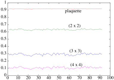
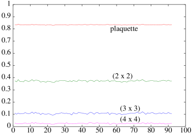
Figure 1: HYP smeared (l.h.s.) and stout smeared (r.h.s.) Wilson loops of different sizes. Note that for a $(4\times 4)$ Wilson loop the expectation value of the HYP smeared loop is $\sim$ 5 times larger than the stout smeared one. (Data from run on line 2 in Table 1.)

As a first indicator we set the scale on the lattice by using the Sommer parameter. (We may change to using hadron masses at a later stage.) We derive this from HYP smeared Wilson loops of various sizes. Computing the static potential by

$$V(r)=-\frac{1}{T_{2}-T_{1}}\,\log\left[\frac{W(r,T_{2})}{W(r,T_{1})}\right]\;.$$ (1)

and assuming the usual form of the potential $V(r)=\sigma r+\mu+c/r$, we obtain the parameters $\sigma,\,\mu$ and $c$ by fitting. Then the Sommer parameter is as usual given by $r_{0}^{2}F(r_{0})=1.65$, which in this case translates to $r_{0}=\sqrt{(1.65+c)/\sigma}$. To set the scale explicitly in fermi we use $r_{0}=0.5$ fm. The sizes of the Wilson loops are such that $r_{0}$ lies inside the range of $r$ used in the fits.

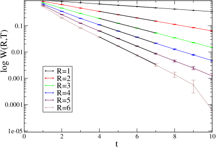
Figure 2: Sommer parameter ($r_{0}$) using HYP smeared Wilson loops. $8^{3}\times 16$ lattice with lattice spacing $a=0.135$ fm and bare quark mass $m_{q}=0.05$ in units of $a$.

To make sure that the lattice spacing obtained in this way (cf. Table 1) does not depend on the smearing procedure, we repeated the calculation with stout smearing. That reproduced the results, albeit with slightly larger error bars.

3 Results

$L^{3}\times T$	$a\,m$	$\beta_{\textrm{\scriptsize{LW}}}$	$res$	$\Delta t$	steps	acc.	HMC	$a$[fm]
							time
$8^{3}\times 16$	0.05	5.4	$10^{-10}$	0.015	50	$\sim$93%	700	0.114(3)
$8^{3}\times 16$	0.05	5.3	$10^{-10}$	0.015	50	$\sim$91%	700	0.135(3)
$8^{3}\times 16$	0.08	5.4	$10^{-10}$	0.015	50	$\sim$93%	700	0.138(3)
$12^{3}\times 24$	0.05	5.3	$10^{-8}$	0.01	100	$\sim$87%	200	0.129(3)

Table 1: Parameters, statistics and some results from our dynamical simulations.

In Table 1 we summarize our run parameters. More details are given in [5].

Next we look at the correlators of the two lightest mesons, the $\pi$ and the $\rho$ mesons. Here we measure only point-to-point correlators defined by

$$C_{\pi}(0,t) = \sum_{\vec{x}}\;\textrm{tr}\left(\gamma_{5}\,D_{\textrm{\scriptsize{CI}}}^{-1}({\vec{x}},\,t:0,\,0)\,\gamma_{5}\,D_{\textrm{\scriptsize{CI}}}^{-1}(0,\,0:{\vec{x}},\,t)\right)\;,$$ (2)

$$C_{\rho}(0,t) = \sum_{{\vec{x}},i=1,2,3}\,\;\textrm{tr}\left(\gamma_{i}\;D_{\textrm{\scriptsize{CI}}}^{-1}({\vec{x}},t:0,\,0)\,\gamma_{i}\,D_{\textrm{\scriptsize{CI}}}^{-1}(0,\,0:{\vec{x}},\,t)\right)\;.$$ (3)

To extract the masses, the data were folded about the symmetry point and fitted to the functional form $a\;\cosh[m(t-T/2)]$. For the $8^{3}\times 16$ lattices, there seemed to be some contamination from the higher states and it was not clear if we were indeed observing the asymptotic decays for the correlators (cf. Fig. 3). On $12^{3}\times 24$ lattices, such contaminations were less pronounced and within error bars we seem to obtain the asymptotic decays in the t-ranges shown in the Table 2. In this table we report on the masses for the $\pi$ and the $\rho$ meson as obtained from these correlators determined from fits in the given regions. The errors were obtained from a jackknife analysis. Due to the simple point-like sources the small distance behavior is dominated by excited states. This can be improved by using smeared sources.

Since the $D_{\textrm{\scriptsize{CI}}}$ is only approximately a Ginsparg-Wilson operator, we have to a posteriori confirm that the good chiral properties that we expect are indeed present in the operator. As a cross-check for that we compare the eigenvalue spectrum of $D_{\textrm{\scriptsize{CI}}}$ for several configurations with dynamical fermions with those of a quenched simulation. The spectra have similar “fuzzyness” and are all close to the unit circle, as shown in [5].

For Dirac operators obeying the $\gamma_{5}$ hermiticity, real eigenmodes are the carriers of non-vanishing chirality and enumerate the total net topological charge. For massless exact GW fermions the lowest-lying eigenvalues are all exactly at the zero of the complex plane. For our approximate GW operator, even in the massless case, the lowest-lying eigenvalues are not exactly at zero but have a small real offset. Their total number defines the net topological charge.

lattice-size	$a$(fm)	bare $m_{q}$	t - range	$a\,m_{\pi}$	$\chi^{2}/d.o.f$	$a\,m_{\rho}$	$\chi^{2}/d.o.f$
$8^{3}\times 16$	0.135(3)	0.05	5-8	0.520(15)	$\sim$ 0.4	0.808(14)	$\sim$ 1.5
			6-8	0.500(15)	$\sim$ 0.05	0.776(15)	$\sim$ 0.1
$8^{3}\times 16$	0.114(3)	0.05	5-8	0.598(58)	$\sim$ 0.06	0.881(26)	$\sim$ 0.7
			6-8	0.589(64)	$\sim$ 0.02	0.858(28)	$\sim$ 0.06
$8^{3}\times 16$	0.138(3)	0.08	5-8	0.621(18)	$\sim$ 0.1	0.860(13)	$\sim$ 1.3
			6-8	0.611(23)	$\sim$ 0.01	0.839(17)	$\sim$ 0.1
$12^{3}\times 24$	0.129(3)	0.05	7-10	0.384(21)	$\sim$ 0.08	0.575(37)	$\sim$ 0.01
			8-10	0.366(26)	$\sim$ 0.04	0.575(15)	$\sim$ 0.06

Table 2: $\pi$ and $\rho$ masses (in lattice units) from point to point correlators

Figure 3: $\rho\,(\ast\,,\,\Box)$ and $\pi\,(\triangle\,,\,\times)$ correlators on $8^{3}\times 16$ lattices ($a\,m_{q}=0.05$). The upper line corresponds to lattice spacing $a=0.135$ fm while the lower one is for $a=0.114$ fm in both channels.

It is important to determine the amount of autocorrelation present in the system. This is explored in [5]. Here we look at another closely related question, whether the algorithm samples all topological sectors of our model in the right way. We show a history of the number of close-to-zero modes (i.e., the absolute value of the topological charge) and symmetrized histogram of the topological charge (it is symmetrized simply because we did not compute the chirality of our real modes) in Fig.  4. Data taken from different Markov chains are separated by dashed lines in the figure. We do observe tunneling (which seems to be a problem for the overlap operator) and a Gaussian-like shape of the distribution.

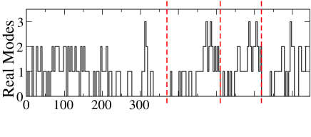
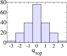
Figure 4: History of real modes and symmetrized histogram of the topological charge.

Figure 5: Distribution of “spatial” Wilson lines for $8^{3}\times 16$ lattice at $a=$0.135 fm

4 Conclusions

We have successfully implemented HMC with the chirally improved Dirac operator and our first results seem to indicate that the good chiral properties which were observed in the quenched case seem to be present in the dynamical case also. In contrast to the overlap operator, we do not have a strong barrier at the topological boundaries and we see quite often evidence of tunneling, manifested as “zero modes” of the $D_{\textrm{\scriptsize{CI}}}$. We also confirm (Fig. 5) that we have not undergone spatial deconfinement by looking at Wilson lines along any one of the shorter directions of the lattice.

We estimate the masses of the $\pi$ and $\rho$ meson using point-to-point correlators. From quenched calculations [3] we know that $8^{3}\times 16$ lattices (at $a=$0.15 fm) still have substantial size dependence and we expect the same to hold here too. However, the $12^{3}\times 24$ lattices ($\sim 1.5$ fm) should be better behaved. In this exploratory study we are at comparatively heavy quark masses $m_{\pi}/m_{\rho}\approx 0.6$. Runs using lighter masses are in progress.

References

- [1] C. Gattringer, A new approach to Ginsparg-Wilson fermions, Phys. Rev. D 63 (2001) 114501 [hep-lat/0003005].
- [2] C. Gattringer, I. Hip, and C. B. Lang, Approximate Ginsparg-Wilson fermions: A first test, Nucl. Phys. B 597 (2001) 451 [hep-lat/0007042].
- [3] C. Gattringer, M. Göckeler, P. Hasenfratz, et. al., Quenched spectroscopy with fixed-point and chirally improved fermions, Nucl. Phys. B 677 (2004) 3 [hep-lat/0307013].
- [4] C. Morningstar and M. Peardon, Analytic smearing of SU(3) link variables in lattice QCD, Phys.Rev. D 69 (2004) 054501 [hep-lat/0311018].
- [5] C. B. Lang, P. Majumdar and W. Ortner, Implementing dynamical chirally improved fermions in lattice qcd, these proceedings, PoS(LAT2005)124.