Lattice calculation of low energy constants with Ginsparg-Wilson type fermions

Abstract

We present a quenched lattice calculation of low energy constants using the chirally improved Dirac operator. Several lattice sizes at different lattice spacings are studied. We systematically compare various methods for computing these quantities, using pseudoscalar and axial vector correlators. We find consistent results for the different approaches, giving rise to $f_{\pi}=96(2)(4)\;\textrm{MeV}$, $f_{K}=106(1)(8)\;\textrm{MeV}$, $f_{K}/f_{\pi}=1.11(1)(2)$, $\Sigma=-(286(4)(31)\;\textrm{MeV})^{3}$, the average light quark mass $\bar{m}=4.1(2.4)\;\textrm{MeV}$ and $m_{s}=101(8)\;\textrm{MeV}$.

I Introduction and Motivation

Low energy theorems were derived quite early in the study of hadrons. When QCD was accepted as a prime candidate for the underlying quantum field theory it became clear that its (approximate) chiral flavor symmetry is spontaneously broken. One may use the corresponding ground state as a starting point for a systematic expansion (Chiral Perturbation Theory, ChPT) taking into account the explicit symmetry violations due to small masses of the light quarks. In such an expansion phenomenological parameters, the so-called low energy constants, have to be determined independently.

The leading order low energy parameters like the pion decay constant or the quark condensate are well-known from “classical” low energy theorems and experiments. It is a challenge, however, to find these parameters based exclusively on ab-initio calculations for QCD. Of course also QCD has its minimal set of input parameters (fixing the scale and the quark masses), but except for these, all other properties can, at least in principle, be derived. Due to the special nature as a strongly interacting quantum field theory only non-perturbative calculations lead to that numbers. The lattice formulation appears to be the prime approach for that aim, using a non-perturbative computer evaluation of the QCD path integral.

For a long time the lattice approach has been plagued by the problem of incorporating chiral symmetry in the fermionic action. It took almost two decades from the first numerical results for lattice gauge theory before it was understood how chiral symmetry may be formulated on the lattice. The Ginsparg-Wilson condition (GWC) GiWi82 , characterizes the class of Dirac operators allowing for the lattice analog of chiral symmetry Lu98 . The Dirac operators obeying the GWC exactly NaNe93a ; NaNe95 ; Ne98 ; Ne98a or approximately Ka92 ; FuSh95 ; HaNi94 ; Ga01 ; GaHiLa00 allow one to approach smaller quark masses than with the more traditional Wilson fermions.

However, the GW-fermions need additional effort for their numerical implementation. Overlap fermions, which obey the GWC exactly, are almost two orders of magnitude more expensive in terms of computer power than Wilson fermions. The approximate GW-fermions are cheaper, but still one order of magnitude more expensive. For that reason there are only few first attempts to use these Dirac operators for a simulation of full QCD with dynamical quarks. There are, however, several results for the quenched case.

In GaGoHa03a hadron masses in the quenched case have been studied for two types of Dirac operators that obey the Ginsparg-Wilson relation to a good approximation: the fixed point operator and the chirally improved operator. Due to their good chiral behavior, these fermions provide a suitable framework for the calculation of low energy constants. Since such a calculation involves quantities that are renormalized, one also has to determine renormalization constants for the connection with a continuum scheme like $\overline{\textrm{MS}}$. Whereas in the case of the overlap action there are exact symmetries relating the renormalization constants of the scalar with the pseudoscalar and the vector with the axial vector sectors, for fermions with only approximate GW-symmetry such relations have to be checked, too.

For the overlap action there have been several determinations of low energy parameters GiHoRe01E ; GiHoRe02 ; BaBeGa05 ; GiLuWe03 ; ChHs03 ; GiHeLa0304 ; DoDrHo02 ; DrDoHo03a ; HeJaLe99 ; HaHaJo02 ; WeWi05 ; BiSh05 ; DuHo05 . For the chirally improved Dirac operator $D_{\textrm{\scriptsize CI}}$ only preliminary results have been published GaGoHa03b ; GaGoHa03a . The reason was, that the renormalization constants were not available. Meanwhile the necessary constants for quark bilinears have been determined for $D_{\textrm{\scriptsize CI}}$ in GaGoHu04 . This now allows us to compute some of the basic low energy parameters in the quenched case. For this purpose we study quenched QCD at various values of the quark masses and determine results for $m_{u}=m_{d}\neq m_{s}$ in the $u\overline{d}$ and $u\overline{s}$ meson sector for several lattice sizes and lattice spacings, down to a pion mass of 330 MeV. Our gauge action is the Lüscher-Weisz action LuWe85 .

In Sect. II we fix our notation and recapitulate the basic relations like PCAC, the axial Ward identity and the Gell’Mann-Oakes-Renner (GMOR) relation. We then discuss the observables used in our analysis. In Sect. III we discuss the details of the lattice simulation and present the results for the masses and low energy parameters (like the meson and quark masses, meson decay constants, chiral condensate) in Sect. IV. We summarize and conclude in Sect. V.

II Low energy constants and their relations

All of the relations are given for Euclidean space-time. We first introduce our notation and then briefly summarize the three key relations which we need in our extraction of low energy constants from lattice simulations. A collection of the relevant vacuum expectation values and ratios thereof ends this section.

II.1 Basic definitions and relations

For flavor symmetry group SU(2) we define the unrenormalized (lattice) isovector operators for the pseudoscalar, vector and axial vector sector through (all fields are taken at the same space-time point)

$$P^{a} = \frac{1}{2}\,\overline{\psi}\,\gamma_{5}\,\tau^{a}\,\psi\;,$$ (1)

$$V_{\mu}^{a} = \frac{1}{2}\,\overline{\psi}\,\gamma_{\mu}\,\tau^{a}\,\psi\;,$$ (2)

$$A_{\mu}^{a} = \frac{1}{2}\,\overline{\psi}\,\gamma_{\mu}\,\gamma_{5}\,\tau^{a}\psi\;.$$ (3)

The fermion fields are flavor doublets $\psi=(u,\,d)$ and $\tau^{a},a=1,2,3$ are the Pauli-matrices. Charged quark bilinear operators are defined through, e.g.,

$$P^{+}=\frac{1}{2}\,\overline{\psi}\,\gamma_{5}\,(\tau^{1}-\mathrm{i}\,\tau^{2})\,\psi=\overline{d}\,\gamma_{5}\,u\;.$$ (4)

Quantities renormalized according to a continuum renormalization scheme are denoted with a superscript $(r)$. As our reference scheme we use the $\overline{\textrm{MS}}$-scheme at a scale of $\mu=2$ GeV. The renormalized quantities are related to their lattice counterparts via renormalization constants,

$$P^{(r)a} = Z_{P}\,P^{a}\;,$$ (5)

$$V_{\mu}^{(r)a} = Z_{V}\,V_{\mu}^{a}\;,$$ (6)

$$A_{\mu}^{(r)a} = Z_{A}\,A_{\mu}^{a}\;,$$ (7)

$$m^{(r)} = Z_{m}\,m\;,$$ (8)

$$\Sigma^{(r)} = Z_{S}\,\Sigma\;\;\textrm{with}\;\;Z_{S}=1/Z_{m}\;.$$ (9)

Here $m^{(r)}$ denotes the renormalized quark mass and $\Sigma^{(r)}$ the renormalized condensate, where the bare condensate reads

$$\Sigma\equiv\frac{1}{2}\langle\overline{u}u+\overline{d}d\rangle\;.$$ (10)

The renormalization constants relate different schemes. For exactly chirally symmetric actions we would have $Z_{S}=Z_{P}$ and $Z_{V}=Z_{A}$. The chirally improved Dirac action used here is only approximately chirally symmetric and we have computed the renormalization factors (in the chiral limit) in GaGoHu04 , utilizing the non-perturbative methods suggested in MaPiSa95 ; GoHoOe99 .

We now discuss the basic relations in terms of renormalized quantities (measurable experimentally and defined in the $\overline{\textrm{MS}}$-scheme). The axial vector current is related to the vector current by commutation relations in current algebra. For conserved vector currents the normalization is therefore fixed for both. The axial vector operator couples to the weak interaction currents. Its relation to the physical (renormalized) isovector pion field defines the pion decay constant, i.e.,

$$\partial_{\mu}A^{(r)a}_{\mu}=M_{\pi}^{2}\,f_{\pi}\,\phi^{(r)a}\;.$$ (11)

(There are also other conventions differing by, e.g., a factor of $\sqrt{2}$. Our definition corresponds to an experimental value of 92.4(3) MeV PDBook04 .) The (renormalized) pion field obeys ($x=(\vec{x},\,t)$)

$$\langle 0|\,\phi(x)^{(r)a}\,|{\pi^{b}(\vec{p}=0)}\rangle=\delta_{ab}\,\mathrm{e}^{-M_{\pi}\,t}\;.$$ (12)

Various equivalent expressions for expectation values may be derived, in particular the so-called partially conserved axial vector current (PCAC) relation:

$$\partial_{\mu}\langle 0|\,A^{(r)a}_{\mu}(x)\,|{\pi^{b}(\vec{p}=0)}\rangle=\delta_{ab}\,M_{\pi}^{2}\,f_{\pi}\,\mathrm{e}^{-M_{\pi}\,t}\;.$$ (13)

Global symmetries of an action at the classical level lead to conserved Noether currents. In a quantum field theory global symmetries of the action are expected to manifest themselves by an analog to the conservation of Noether currents. To derive these relations one considers infinitesimal symmetry transformations of the fermion fields in the path integral

$$\langle 0|{\cal O}|0\rangle=\frac{1}{Z}\int dU\,d\bar{\psi}\,d\psi\,\;{\cal O}[U,\bar{\psi},\psi]\;e^{-S[U,\bar{\psi},\psi]}\;,$$ (14)

where ${\cal O}$ denotes an arbitrary operator. Some classical symmetries may be spontaneously broken or broken due to anomalies resulting from the functional integration. If the integration measure is invariant under the transformation this lead to (Ward-) identities of the form

$$\langle 0|\delta{\cal O}|0\rangle-\langle 0|{\cal O}\delta S|0\rangle=0\;.$$ (15)

Thus, the quantum analog to the classical conservation law has similar (or equal, ${\cal O}=1$) form, but is an operator identity.

For the QCD Lagrangian (renormalized, e.g., in the $\overline{\textrm{MS}}$-scheme) one exploits the invariance properties under symmetry transformations to derive Ward identities. Although obtained first on the classical level and on-shell, the relations hold under quantization and one ends up with local operator identities for the full quantized theory. (For the singlet axial vector there is an additional anomaly contribution from the integration measure.)

In the quark sector chiral symmetry is broken explicitly by the quark mass matrix ${\cal M}$ and one finds

$$\partial_{\mu}V^{(r)a}_{\mu} = \frac{1}{2}\,\left(\overline{\psi}[\tau^{a},{\cal M}]\psi\right)^{(r)}\;,$$ (16)

$$\partial_{\mu}A^{(r)a}_{\mu} = \frac{1}{2}\,\left(\overline{\psi}\gamma_{5}\{\tau^{a},{\cal M}\}\psi\right)^{(r)}\;.$$ (17)

If the quark masses are degenerate, the vector current is conserved and the axial vector current obeys the axial Ward identity (AWI),

$$\partial_{\mu}A^{(r)a}_{\mu}=2\,m^{(r)}\,P^{(r)a}\;.$$ (18)

Combining this with relation (11) gives

$$2\,m^{(r)}\,P^{(r)a}=f_{\pi}\,M_{\pi}^{2}\phi^{a}\;.$$ (19)

The correlation function of the normalized pion field (cf. (12)) reads

$$\langle 0|\phi^{(r)a}(\vec{p}=0,t)\phi^{(r)b}(0)|0\rangle=\frac{1}{2\,M_{\pi}}\,\delta_{ab}\,\mathrm{e}^{-M_{\pi}\,t}\;.$$ (20)

The asymptotic behavior of the pseudoscalar field correlator

$$\langle 0|P^{(r)a}(\vec{p}=0,t)P^{(r)b}(0)|0\rangle=(G_{\pi}^{(r)})^{2}\,\frac{1}{2\,M_{\pi}}\,\delta_{ab}\,\mathrm{e}^{-M_{\pi}\,t}\;,$$ (21)

is dominated by the pion state as well. We have introduced the relative factor $G_{\pi}^{(r)}$, which, from (19), is

$$|\langle 0|P^{(r)}|\pi(\vec{0})\rangle|=G_{\pi}^{(r)}=\frac{f_{\pi}\,M_{\pi}^{2}}{2\,m^{(r)}}\;.$$ (22)

Another Ward identity may be derived taking ${\cal O}=P$, leading to

$$\Sigma^{(r)}=-\frac{m^{(r)}}{M_{\pi}^{2}}|\langle 0|P^{(r)}|\pi(\vec{0})\rangle|^{2}\;,$$ (23)

where we assume degenerate light quark masses for simplicity. This, combined with the definition of the pion decay constant and (19), leads to the usual form of the GMOR relation:

$$f_{\pi}^{2}\,M_{\pi}^{2}=-2\,m^{(r)}\,\Sigma^{(r)}\;.$$ (24)

The exploitation of the underlying principles has then led to the development of chiral perturbation theory We79 ; GaLe84 . In that context a systematic expansion of many observables in terms of low energy constants has been derived. These constants, however, have to be determined either from experiment or from basic principles, i.e., non-perturbative solution of the underlying field theory QCD. The lattice formulation of QCD allows such a determination.

II.2 Lattice relations

Let us now express the renormalized quantities through their lattice counterparts, using the relations (5) – (9). Since we need to avoid the evaluation of disconnected diagrams we restrict ourselves to the isovector charged bilinears

$$\frac{1}{2}\,\overline{\psi}\,\Gamma\,(\tau^{1}-\mathrm{i}\,\tau^{2})\,\psi=\overline{d}\,\Gamma\,u\;,$$ (25)

where $\Gamma$ is $\gamma_{5},\gamma_{\mu}$ or $\gamma_{\mu}\gamma_{5}$. Consequently from now on we drop the flavor superscript $a$.

In the simulations we always keep the quark sources (and thus the operator source) at a fixed time $t=0$ and compute propagators to all other lattice points. We sum over the spatial volume of the sink time slice in order to project to zero spatial momentum $\vec{p}=0$.

Taking into account the renormalization factors, the following correlators of lattice operators and ratios have been studied ($\mu=4$ refers to the Euclidean time direction, the symbol $\sim$ denotes the asymptotic behavior for large $t$):

$$Z_{P}^{2}\,\langle P(\vec{p}=0,t)P(0)\rangle \sim \frac{(G_{\pi}^{(r)})^{2}}{M_{\pi}}\,\mathrm{e}^{-M_{\pi}\,t}$$ (26)

$$= \frac{f_{\pi}^{2}M_{\pi}^{3}}{4\,(m^{(r)})^{2}}\,\mathrm{e}^{-M_{\pi}\,t}$$

$$= \frac{M_{\pi}\,|\Sigma^{(r)}|}{2\,m^{(r)}}\,\mathrm{e}^{-M_{\pi}\,t}\;,$$

$$Z_{A}\,Z_{P}\,\langle\,A_{4}(\vec{p}=\vec{0},t)\,P(0)\rangle \sim G_{\pi}^{(r)}\,f_{\pi}\,\mathrm{e}^{-M_{\pi}\,t}$$ (27)

$$= \frac{f_{\pi}^{2}\,M_{\pi}^{2}}{2\,m^{(r)}}\,\mathrm{e}^{-M_{\pi}\,t}$$

$$= |\Sigma^{(r)}|\,\mathrm{e}^{-M_{\pi}\,t}\;,$$

$$Z_{A}\,Z_{P}\,\langle\,\partial_{t}A_{4}(\vec{p}=\vec{0},t)\,P(0)\rangle \sim G_{\pi}^{(r)}\,f_{\pi}\,M_{\pi}\,\mathrm{e}^{-M_{\pi}\,t}$$ (28)

$$= \,\frac{f_{\pi}^{2}\,M_{\pi}^{3}}{2\,m^{(r)}}\,\mathrm{e}^{-M_{\pi}\,t}$$

$$= |\Sigma^{(r)}|\,M_{\pi}\,\mathrm{e}^{-M_{\pi}\,t}\;,$$

$$Z_{A}^{2}\,\langle\,A_{4}(\vec{p}=\vec{0},t)\,A_{4}(0)\rangle \sim M_{\pi}\,f_{\pi}^{2}\,\mathrm{e}^{-M_{\pi}\,t}\;,$$ (29)

$$Z_{A}^{2}\,\langle\,\partial_{t}A_{4}(\vec{p}=\vec{0},t)\,A_{4}(0)\rangle \sim M_{\pi}^{2}\,f_{\pi}^{2}\mathrm{e}^{-M_{\pi}\,t}\;,$$ (30)

$$Z_{A}\,Z_{P}\, \sqrt{\langle\,A_{4}(\vec{p}=\vec{0},t)\,A_{4}(0)\rangle\,\langle\,P(\vec{p}=\vec{0},t)\,P(0)\rangle}$$ (31)

$$\hskip 82.51299pt\sim|\Sigma^{(r)}|\,\mathrm{e}^{-M_{\pi}\,t}\;.$$

The pseudoscalar masses thus may be derived from the exponential decay and the other low energy parameters from its coefficient. We cannot use correlators like $\langle(\partial_{t}A_{4}(t))(\partial_{t}A_{4}(0))\rangle$ since the source is fixed to the time slice $t=0$ and thus we cannot construct the lattice derivative there.

The asymptotic behavior cancels in the following ratios:

$$\frac{Z_{A}}{Z_{P}}\,\frac{\langle\,\partial_{t}A_{4}(\vec{p}=\vec{0},t)\,X(0)\,\rangle}{\langle\,P(\vec{p}=\vec{0},t)\,X(0)\,\rangle} \sim \frac{M_{\pi}^{2}\,f_{\pi}}{G_{\pi}^{(r)}}$$ (32)

$$= Z_{m}\,2\,m=2\,m^{(r)}\;,\;\;$$

where $X$ may be $P$ or $A_{4}$. Further useful ratios are

$$\frac{Z_{A}}{Z_{P}}\,\frac{\langle\,A_{4}(\vec{p}=\vec{0},t)\,P(0)\,\rangle}{\langle\,P(\vec{p}=\vec{0},t)\,P(0)\,\rangle} \sim \frac{M_{\pi}\,f_{\pi}}{G_{\pi}^{(r)}}=Z_{m}\,\frac{2\,m}{M_{\pi}}$$ (33)

$$= \frac{2\,m^{(r)}}{M_{\pi}}=\frac{M_{\pi}f_{\pi}^{2}}{|\Sigma^{(r)}|}\;,$$

$$\frac{Z_{A}^{2}}{Z_{P}^{2}}\,\frac{\langle\,A_{4}(\vec{p}=\vec{0},t)\,A_{4}(0)\,\rangle}{\langle\,P(\vec{p}=\vec{0},t)\,P(0)\,\rangle} \sim \left(\frac{\,M_{\pi}\,f_{\pi}}{G_{\pi}^{(r)}}\right)^{2}$$ (34)

$$= \left(\frac{\,M_{\pi}\,f_{\pi}^{2}}{\Sigma^{(r)}}\right)^{2}$$

$$= \left(\frac{2\,m^{(r)}}{M_{\pi}}\right)^{2}\;,$$

$$\frac{Z_{P}}{Z_{A}}\,\frac{\langle\,\partial_{t}A_{4}(\vec{p}=\vec{0},t)\,P(0)\,\rangle}{\langle\,A_{4}(\vec{p}=\vec{0},t)\,A_{4}(0)\,\rangle} \sim \frac{G_{\pi}^{(r)}}{f_{\pi}}=\frac{M_{\pi}^{2}}{2\,m^{(r)}}\;,$$ (35)

$$\frac{\langle\,\partial_{t}A_{4}(\vec{p}=\vec{0},t)\,P(0)\,\rangle^{2}}{\langle\,A_{4}(\vec{p}=\vec{0},t)\,A_{4}(0)\,\rangle\langle\,P(\vec{p}=\vec{0},t)\,P(0)\,\rangle} \sim M_{\pi}^{2}\;.\;\;$$ (36)

Ratios involving the lattice derivative $\partial_{t}A_{4}$ depend on the way the derivative is taken. Details will be discussed in Subsection III.3.

Due to lattice periodicity and the parity properties of the meson propagators, the exponential term $\exp{(-M\,t)}$ is accompanied by another term from the propagation backwards in time, $\exp{(-M\,(T-t))}$. Depending on the correlation function we therefore observe $\cosh$- (for $\langle PP\rangle$ and $\langle A_{4}A_{4}\rangle$ correlators) or $\sinh$-behavior (for $\langle A_{4}P\rangle$ and $\langle(\partial_{t}A_{4})A_{4}\rangle$ correlators).

III Technicalities

III.1 Setup

In the fermion action we use the chirally improved Dirac operator $D_{\textrm{\scriptsize CI}}$  Ga01 ; GaHiLa00 . It is based on a systematic expansion of the lattice Dirac operator taking into account the whole Clifford algebra and terms coupling fermions within a certain range of neighbors on the lattice. The expanded Dirac operator is inserted in the GWC which then leads to a set of algebraic equations for the expansion coefficients. The equations include a normalization condition, which depends on the lattice spacing and thus on the gauge action. The solution of the system of algebraic equations gives the coefficients defining $D_{\textrm{\scriptsize CI}}$. In recent applications GaGoHa03a , as well as here, we use a set of 19 independent terms in the expansion in the action. Taking into account the lattice symmetries this then corresponds to several hundred coupling terms at each site of the lattice. Finally, in the definition of $D_{\textrm{\scriptsize CI}}$  also one step of HYP-smearing of the gauge configuration is included HaKn01 . For the gauge fields we use the Lüscher-Weisz action LuWe85 . The lattice spacings have been determined using the Sommer parameter GaHoSc02 . We summarize the simulation parameters in Table 2.

The strange quark mass parameter was set using the kaon mass (chiral extrapolation with non degenerate quark masses). This gives a value Ha05a of $a\,m_{s}=0.089(2)$ for $\beta=7.90$ and $a\,m_{s}=0.061(1)$ for $\beta=8.15$. For $\beta=8.15$ we have quark propagators at $a\,m=0.06$ and we used those for the strange quark. For $\beta=7.90$ we have quark propagators for $am=0.08$ and $a\,m=0.10$. We interpolate the hadron results from those two values to the strange quark mass at $a\,m=0.089$. All results for the $K$-meson are based on quark propagators with non-degenerate quark masses. In the discussion the corresponding meson fields, however, will still be called $P$ and $A$ in order to simplify our notation.

The necessary renormalization constants for fermionic bilinears were computed in GaGoHu04 and we list them in Table 2 for completeness. All $Z$ are in the chiral limit and for the $\overline{\mbox{MS}}$-scheme at a scale of 2 GeV. The values at $\beta=8.15$ were obtained by interpolation.

Table 1: Parameters of the simulation. Where the strange quark mass is given (in parenthesis), we also determined propagators for strange hadrons. Type denotes the type of the quark source/sink and # cf. the number of configurations entering the analysis.

$L^{3}\times T$	$\beta$	$a[\textrm{fm}]$	$a[\textrm{GeV}^{-1}]$	# cf.	Type	$a\,m$ $(a\,m_{s})$
$8^{3}\times 24$	$7.90$	$0.148$	$0.750$	200	$p,n$	$0.02-0.20$
$12^{3}\times 24$	$7.90$	$0.148$	$0.750$	100	$p,n$	$0.02-0.20$
$12^{3}\times 24$	$8.35$	$0.102$	$0.517$	100	$p,n$	$0.02-0.20$
$16^{3}\times 32$	$7.90$	$0.148$	$0.750$	99	$p,n$	$0.02-0.20$
$16^{3}\times 32$	$8.35$	$0.102$	$0.517$	100	$p,n$	$0.02-0.20$
$16^{3}\times 32$	$8.70$	$0.078$	$0.395$	100	$p,n$	$0.02-0.20$
$16^{3}\times 32$	$7.90$	$0.148$	$0.750$	100	$p,n,w$	$0.02-0.20$
						($0.08,0.10$)
$20^{3}\times 32$	$8.15$	$0.119$	$0.605$	100	$p,n,w$	$0.017-0.16$
						($0.06$)

Table 2: Renormalization constants taken from GaGoHu04 . The values for $\beta=8.15$ have been obtained by interpolation.

$\beta$	$Z_{S}$	$Z_{V}$	$Z_{T}$	$Z_{A}$	$Z_{P}^{\textrm{\scriptsize{Sub}}}$
7.90	1.1309(9)	0.9586(2)	0.9944(3)	1.0087(4)	1.0281(5)
$8.15^{*}$	1.081(1)	0.967(1)	1.014(1)	1.011(1)	1.012(3)
8.35	1.039(1)	0.973(1)	1.028(2)	1.012(1)	0.987(4)
8.70	0.959(2)	0.979(1)	1.049(1)	1.0095(7)	0.915(1)

III.2 Sources and normalization

In order to improve signals we use Jacobi-smeared Gu89 ; BeGoHo97 sources at $t=0$ for the quarks. For most runs we have one smearing width (denoted as $n(arrow)$, cf. Table 2). For some data sets, that have also been used for an analysis of the excited hadron masses BuGaGl04a , we have two different widths ($n$ and $w(ide)$). In addition we also use point-like sinks ($p(oint)$) for sake of normalizing our results as discussed below. The smearing widths are chosen such that the effective size of a given source is approximately the same for all lattice spacings. The parameters (smearing steps and coupling) thus depend on the gauge coupling BuGaGl04a .

For computing the coefficients of the exponential decay necessary for determining the pion decay constant and the condensate, we have to normalize the hadron sources to point-like bilinears. Our normalization procedure is set up as follows: Let us denote by $X_{s_{1}s_{2}}$ a mesonic operator built out of an anti-quark of smearing type $s_{1}$ and a quark of smearing type $s_{2}$ with $s_{i}=n,w$ or $p$. Guided by the arguments discussed below we find that we may safely assume factorization of the normalization factors,

$$X_{s_{1}s_{2}}=C_{s_{1}}^{X}\,C_{s_{2}}^{X}\,X_{pp}\;.$$ (37)

For ratios like

$$\frac{\langle X_{s_{1}s_{2}}X_{s_{3}s_{4}}\rangle}{\langle X_{s_{1}s_{2}}X_{pp}\rangle}\;,$$ (38)

we find excellent plateaus for $t,\,t^{\prime}\in[t_{a},t_{b}]=[4,\,T-4]$ and violations of the factorization hypothesis (37) smaller than 1.2 % for the narrow and wide results at $\beta=7.90$, and less than 2.2 % for the results at $\beta=8.15$. In this way we obtain numbers for $(C_{n}^{X})^{2}$, $(C_{w}^{X})^{2}$ and $C_{n}^{X}C_{w}^{X}$ and from them find the values for $C_{n}^{X}$, $C_{w}^{X}$. The coefficients are calculated for all operators $X$, and separately for each gauge coupling, volume and quark mass. For the large physical volumes we find very little ${\cal O}(1\%)$ dependence of the $C_{s}^{X}$ on the quark mass which increases for the smallest volumes to a variation of ${\cal O}(5-10\%)$ over the range of quark masses we consider. The relative statistical errors from the plateau fits are less than 0.0005 and were neglected in the further analysis.

As a consistency check we compared the final results for all possible smearing combinations and checked whether the resulting masses and in particular the prefactors of the exponential decay are in agreement when normalized appropriately. This was the case and in the subsequent presentation we therefore do not discuss this issue any more. All results presented here are based on the results with narrow quark sources.

III.3 Fits, error estimates and numerical derivatives

Fitting procedure: At larger $t$, where excited state contributions become negligible, the propagators have a $\cosh$ or $\sinh$ functional behavior. Therefore we may extract the prefactor $D$ and the meson mass $M$ performing a correlated least-squares fit of the correlation function $C(t)$ to

$$D(M)\,f(M,\,t)\quad\textrm{with}\quad f(M,\,t)\equiv\left(\mathrm{e}^{-M\,t}\pm\mathrm{e}^{-M\,(T-t)}\right)\;,$$ (39)

by minimizing

$$\chi^{2} = \sum_{t,t^{\prime}}\Big{[}C(t)-D(M)\,f(M,\,t)\Big{]}\,\mathrm{Cov}^{-1}(t,\,t^{\prime})$$ (40)

$$\;\;\;\times\,\Big{[}C(t^{\prime})-D(M)\,f(M,\,t^{\prime})\Big{]}\;.$$

Here $\mathrm{Cov}$ denotes the covariance matrix for the correlation function entries and $t,\,t^{\prime}\in[t_{a},t_{b}]$. The minimization may be simplified by observing, that for given $M$ the minimum of $\chi^{2}$ is obtained for

$$D(M)=\frac{\sum_{t,t^{\prime}}\;C(t)\,\mathrm{Cov}^{-1}(t,t^{\prime})\,f(M,\,t^{\prime})}{\sum_{t,t^{\prime}}\;f(M,\,t)\,\mathrm{Cov}^{-1}(t,t^{\prime})\,f(M,t^{\prime})}\;.$$ (41)

Using this relation one performs the one-dimensional minimization of (40) with regard to $M$.

Ratios of correlation functions are fitted to constants in $t\in[t_{a},t_{b}]$.

Error estimation: The correlator values are arranged in overlapping blocks according to the standard jackknife algorithm. Each block consists of typically 95% of all hadron propagators for a given set of lattice parameters.

For each such jackknife block we then determine the values of the propagator and the requested ratios at various $t$, as well as the covariance matrix for the propagator and the variance for the ratios. These are then fitted as discussed, i.e., either to asymptotic $\cosh$- or $\sinh$-behavior or to a constant. For this fit the relative weights (as defined from the covariance and variance) are important.

We also need variances for the correlators involving derivatives with regard to $t$ (discussed below), as they also enter some of the ratios. Since we need these for each jackknife set we estimate the variance of the derivatives by performing another jackknife analysis within the given set.

The fits (and the extrapolations to the chiral limit) are then repeated for all jackknife blocks and the variation of the results for coefficients, mass values and ratios leads to the estimate for the corresponding errors.

Numerical derivatives: For some of the ratios of correlators we need derivatives of the correlator with regard to time $t$. Numerical derivatives are always based on assumptions on the interpolating function. Usual simple 2- or 3-point formulas assume polynomials as interpolating functions. We can do better by utilizing the information on the expected $\cosh$- and $\sinh$-dependence. In fact, we may use these functions for local 3-point interpolation and get the derivative therefrom.

A 2-point derivative based only on function values $y_{t}$ and $y_{t-1}$ is not suitable since it provides values at half-integer $t$. We therefore use a local 3-point fit to $y_{t-1}$, $y_{t}$ and $y_{t+1}$ to the functional form (39) (depending on whether the correlator is symmetric or anti-symmetric in $t$), where the parameters $\overline{D}$ and $\overline{M}$ now depend on the actual value of $t$. We then reconstruct the derivative as

$$\partial_{t}f(\overline{M},\,t)\equiv\overline{M}\left(-\mathrm{e}^{-\overline{M}\,t}\pm\mathrm{e}^{-\overline{M}\,(T-t)}\right)\;.$$ (42)

Then the desired ratios can be computed in a straightforward manner and the plateau values obtained by fits.

When analyzing not ratios but the correlators of type $\langle(\partial_{t}A_{4})X\rangle$ directly, we perform a global fit to $\langle A_{4}X\rangle$ according to (39) and take the analytic derivative.

IV Results

Throughout the analysis we refer to the quantities as defined in Sect. II.2. Where we give physical, renormalized ($\overline{\textrm{MS}}$-scheme) values we always use the renormalization factors as obtained in the chiral limit, even in plots for non-vanishing bare quark masses. The renormalization factors $Z$ relate to the continuum $\overline{\textrm{MS}}$-scheme at a scale of $\mu=2\;$GeV and are $a$-dependent as given in Table 2.

IV.1 Meson Masses

In Fig. 1 we present results for the pseudoscalar masses as determined from the exponential fit of the $A_{4}$-correlator (29) for the time components of the axial vector. The kaon propagators are determined from the same interpolators but for non-degenerate quark masses. The translation of results in lattice units to physical mass values was done using the values for the lattice constant $a$ given in Table 2. It is interesting to note that the linear extrapolation of our pion mass results implies a small residual quark mass. We remark that when using the pseudoscalar correlator at $\beta=7.90$ and an extrapolation formula inspired by quenched chiral perturbation theory (QChPT) BeGo92 ; Sh92 ; BeGo94 no such effect was observed GaGoHa03a .

The value of the strange quark mass has been chosen such that the kaon mass agrees with experiment at the linear extrapolation in the light quark mass to the physical point. For the $16^{3}\times 32$ lattice at $\beta=7.90$ we interpolate $M_{K}^{2}$ linearly between the two values of the strange quark mass neighboring the physical point at $a\,m_{s}=0.089$, cf. Fig. 2.

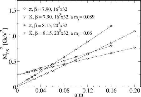
Figure 1: $M_{\pi}^{2}$ and $M_{K}^{2}$ determined from the asymptotic behavior of the $A_{4}$-correlator (29).

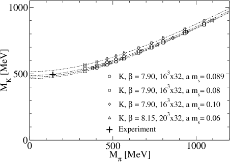
Figure 2: $M_{K}$ vs. $M_{\pi}$. For the $16^{3}\times 32$ lattice we have interpolated between two values of the strange quark mass; for the $20^{3}\times 32$ lattice $a\,m_{s}=0.06$ corresponds already to the physical point. The curves represent the linear fit in Fig. 1.

Let us now discuss possible sources of systematic errors.

Finite size dependence: In Fig. 3 we compare $a^{2}\,G_{\pi}^{(r)}/Z_{P}$ determined from (26) for $a\,m\geq 0.01$ for three volumes but at the same lattice scale. We find a strong volume dependence for the smallest lattice at bare quark masses below $0.06/a$. This is to be expected since for that quark masses the inverse pion mass becomes larger than half the spatial lattice size. For the larger lattices finite volume effects are significant only for $a\,m<0.02$. We will therefore discuss only results for the large lattices and $a\,m\geq 0.02$ (0.017 for the $20^{3}\times 32$ lattice). The lattices largest in physical units and of similar spatial extent ${\mathcal{O}}(2.4\;\textrm{fm})$ are those of size $16^{3}\times 32$ at $\beta=7.90\,(a=0.148\;\textrm{fm})$ and $20^{3}\times 32$ at $\beta=8.15\,(a=0.119\;\textrm{fm})$.

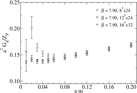
Figure 3: $a^{2}\,G_{\pi}^{(r)}/Z_{P}$ from (26) for $\beta=7.90$ and lattice sizes $8^{3}\times 24$, $12^{3}\times 24$, $16^{3}\times 32$. The finite size significantly affects the small volume data ($8^{3}\times 24$) for $a\,m\leq 0.06$. For the other volumes finite size effects become important for $a\,m<0.02$.

Topological finite size effects: Exact Ginsparg-Wilson Dirac operators have exact zero modes. In quenched simulations these are not suppressed by the fermionic determinant. However, their effects for, e.g., the pion correlators Sh97Sh00 , are hard to detect unless one approaches very small pion masses ${\cal O}(250\;\textrm{MeV})$ DoDrHo04 . For approximate GW-operators like the one studied here the main problem is the (scarce) occurrence of slightly misplaced zero modes, real eigenvalues of $D_{\textrm{\scriptsize CI}}$  below zero. These lead to contributions in the quark propagator that diverge already at some positive, albeit small, mass. The smaller the quark mass parameter is, the stronger one might notice such distortions often referred to as topological finite size effects.

There have been various suggestions to deal with the problem of zero modes in the pseudoscalar propagator BlChCh04 ; GiHoRe01E ; DoDrHo02 ; GaGoHa03a , among them the proposal to study a combination of the iso-non-singlet pseudoscalar and scalar correlators such that the zero modes cancel. Indeed, zero modes contribute differently to different propagators. For exactly chiral Dirac operators for the $A_{4}$-correlator we expect a contribution of $\mathcal{O}(1/m)$, whereas for the $P$-correlator we expect $\mathcal{O}(1/m^{2})$.

In Fig. 4 we show the ratio of pseudoscalar masses obtained from the pseudoscalar and axial propagator ${M_{\pi}(\langle\,P\,P\,\rangle)}/{M_{\pi}(\langle\,A_{4}\,A_{4}\,\rangle)}$, comparing results at two different lattice spacings for the same physical volumes. There are indications for zero mode contributions being stronger for the $P$-correlator on the coarser lattice. For the final pseudoscalar mass values we use the less affected results from the $A_{4}$-correlators.

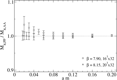
Figure 4: Ratio of the pion masses obtained from the pseudoscalar propagator $\langle PP\rangle$ and the axial propagator $\langle A_{4}A_{4}\rangle$ for the same physical volumes but two different lattice spacings.

Chiral logs: Since quenched QCD does not include the full fermion dynamics, corrections to the chiral expansion introduce new terms, including singular ones (quenched chiral logarithms). On the other hand, it has been hard to clearly identify these in numerical calculations GaGoHa03a ; DoDrHo04 ; BaBeGa05 . In particular, one needs to approach parameter regions, where the pion mass is well below 300 MeV. The situation then is furthermore obscured by the role of zero modes (depending on the fermion action), poor statistics and variation in the fit range.

In quenched chiral perturbation theory (QChPT) BeGo92 ; Sh92 ; BeGo94 one expects for the pseudoscalar mass non-analytic behavior in the quark mass parameter Sh97Sh00 ; HeSoWi00 , which arises from hairpin diagrams and $\eta^{\prime}$ would-be-Goldstone bosons

$$(a\,M_{P})^{2}\propto(a\,m)^{1/(1+\delta)}\;,$$ (43)

where values for $\delta$ ranging from 0.19 to 0.23 have been quoted in recent literature GaGoHa03a ; DoDrHo04 ; BaBeGa05 . In the range of values studied here we cannot disentangle reliably such effects from the possible spurious zero mode contributions and consequently do not attempt to determine $\delta$.

IV.2 Quark masses

In Eq. (32) one utilizes the axial Ward identity to obtain the so-called AWI-mass $m_{\textrm{\scriptsize AWI}}$; the asymptotic exponential behavior of numerator and denominator cancels and thus, including the renormalization factors, this allows one to obtain the renormalized quark mass. In Fig. 5 we plot the results for two choices of the pseudoscalar interpolator $P$, showing the results both in lattice and in physical units.

For the second choice, $X=A_{4}$, the correlators are of $\sinh$-type and therefore the ratio becomes numerically unstable near the symmetry point in $t$. We thus cannot reliably (with small errors) determine the plateau values for this choice if the quark mass parameter is small. However, at all masses where we can compare the two results they are in excellent agreement as may be seen in the figure. The subsequent analysis is based on the more stable choice $X=P$.

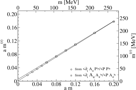
Figure 5: The renormalized quark mass $a\,m^{(r)}$ (in the $\overline{\textrm{MS}}$-scheme) vs. the bare mass parameter $a\,m$ as determined from (32) ($16^{3}\times 32$, $\beta=7.90$) using $X=P$ (squares) and $X=A_{4}$ (circles). For $X=A_{4}$ values at quark masses below $a\,m=0.06$ have been omitted due to unstable plateau fits.

In Fig. 6 we compare the values, again obtained utilizing (32) with $X=P$. The are derived for two different lattice spacings and given in physical units. The lines correspond to linear fits $m^{(r)}\propto M_{\pi}^{2}$, enforcing the simultaneous chiral limit of both observables. The data do not show deviation from that behavior, although logarithmic corrections are expected due to quenching. We observe that the linear extrapolations are in good agreement with the Particle Data Group PDBook04 average for the light quark masses at the physical pion mass. Averaging the extrapolated values obtained at the physical pion mass we obtain an average light quark mass of

$$\frac{1}{2}\left(m_{u}^{(r)}+m_{d}^{(r)}\right)\equiv\bar{m}^{(r)}\simeq 4.1(2.4)\;\textrm{MeV}$$ (44)

in the $\overline{\textrm{MS}}$-scheme. The error is essentially due to the residual quark mass (see Fig.s 6 and 1). The precise determination of this residual quark mass is obscured by the possible contribution of a quenched chiral log (cf. the discussion in GaGoHa03a ). This effect is stronger for the smaller physical volumes and thus we refrain from a determination of $\bar{m}^{(r)}$ for the lattices at $\beta=8.35$ and $8.7$. This prohibits a continuum extrapolation linear in $a$ and we therefore quote the average of the two values for the two lattices with spatial extension 2.4 fm.

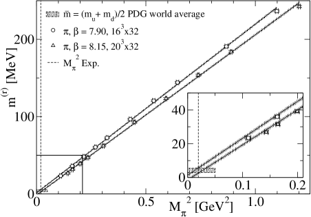
Figure 6: Plot of $m^{(r)}$ (obtained from (32)) vs. $M_{\pi}^{2}$ for two different lattice spacings but similar physical spatial lattice volume. The linear extrapolations are in good agreement with the expected light current quark masses.

As addressed in Sect. III, the bare mass parameter for the strange quark has been fixed such that the kaon mass assumes its physical value when the data are extrapolated to the physical pion mass Ha05a . Fig. 7 compares the results for the corresponding renormalized masses (in lattice units) derived from (32) for kaon and pion correlation functions. For the light quark masses (the pion propagator) the results confirm those of Fig. 5, now for two different lattice spacings superimposed. For the strange quark the fitted lines are close to being parallel with negative intercepts, in good agreement with the negative bare strange quark mass parameters. This again demonstrates that our Dirac operator has very small additive mass renormalization.

For the pion data, the slope of $m^{(r)}$ provides a value for the light quark mass renormalization factor $Z_{m}$. In Table 3 we compare these numbers with the values of $1/Z_{S}$ from GaGoHu04 and find very good agreement. From the PCAC-relation and (32) we expect for the kaon data $a\,m^{(r)}\simeq Z_{m}\,a\,(m_{s}+m)/2$ which is indeed observed.

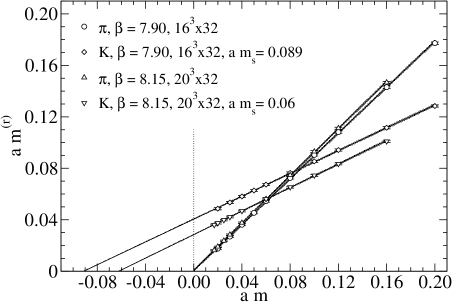
Figure 7: $a\,m^{(r)}$ vs. $a\,m$ from (32) using $X=P$. The slope of $m^{(r)}$ for the pion data provides $Z_{m}$.

Table 3: Renormalization constant $Z_{S}$ from GaGoHu04 (see Table 2) compared to the values of $Z_{m}$ as derived from the slope of the renormalized quark mass.

$\beta$	$a[\textrm{fm}]$	$a[\textrm{GeV}^{-1}]$	$Z_{S}$	$1/Z_{S}$	$Z_{m}$	$Z_{m}Z_{S}$
7.90	0.148	0.750	1.1309(9)	0.8842(7)	0.891(4)	1.007(5)
8.15	0.119	0.605	1.081(1)	0.9250(9)	0.916(5)	0.991(6)

The quark mass data shown in Fig. 8, now in physical units in the $\overline{\textrm{MS}}$-scheme, again give a very consistent picture. Note that now the abscissa gives the corresponding pseudoscalar mass, i.e., that of the pion or the kaon, for the corresponding values of $m^{(r)}$. The error bands show that for given lattice spacing the numbers for kaon and pion are on top of each other, although these states have different quark content. (This justifies the often used strategy to obtain kaon results from pion propagators using degenerate mass quarks.)

Like for the light quark masses in Fig. 6, also the result for the renormalized strange quark mass is in excellent agreement with the world average PDBook04 . Averaging the two values computed at the physical kaon mass for the two lattice spacings we obtain for the strange quark mass

$$\frac{1}{2}\left(m_{s}^{(r)}+\bar{m}^{(r)}\right)\simeq 52(3)\;\textrm{MeV}$$ (45)

in the $\overline{\textrm{MS}}$-scheme. With (44) for the light quarks this then gives $m_{s}^{(r)}=101(8)~{}\textrm{MeV}$. Possible finite size effects and other systematic effects like chiral extrapolation and quenching have not been accounted for. The given error takes into account the standard error and includes the derivations due to the dependence on the lattice spacing. As discussed above for the light quarks, we have only values at two lattice spacings available and therefore cannot perform a sensible continuum extrapolation. Our numbers for the average are in good agreement with determinations from the overlap action in GiHoRe02 ; ChHs03 , and to a less extent also with DuHo05 .

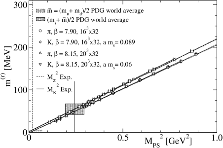
Figure 8: $m^{(r)}$ vs. $M_{PS}^{2}$ from (32) using $X=P$. Here $M_{PS}$ denotes $M_{\pi}$ or $M_{K}$, respectively. All masses are given in physical units in the $\overline{\textrm{MS}}$-scheme.

IV.3 Condensate

For exact GW-fermions the chiral condensate may be obtained from the trace of the inverse Dirac operator. In our case the subtraction constant is not known to sufficient precision and therefore this approach, successfully applied for the overlap operator HeJaLe99 ; HaHaJo02 , does not work Ho04a . Another method uses the density distribution of the small complex eigenvalues; this would be a promising method in our case but it requires the costly determination of the low lying eigenvalue spectrum for all configurations which we did not calculate.

Instead we have computed the renormalized condensate from the relations (24), (27) and (31) which all contain $\Sigma^{(r)}$. The first of these is the GMOR relation, the other two are determinations directly from the coefficients of propagators and implicitly related to GMOR as well. In Figs. 10 and 10 we show our results for $\Sigma^{(r)}$ in lattice units as a function of the bare quark mass. We find excellent agreement for all three determinations. The values are consistent within the error bars.

The dependence on the bare quark mass is compatible with the leading linear chiral behavior. Note, that we are not at small enough quark masses to be in the so-called $\epsilon$-regime but are in the $p$-regime GaLe87a (for recent studies in the $\epsilon$-regime cf. HeJaLe99 ; GiHeLa0304 ; FuHaOk05 ). We show the linear fit (with 1 s.d. error band) to the data from all three types of determination but omit the points with smallest mass value in the fit (cf. our discussion of possible finite size effects).

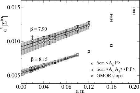
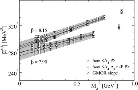
Figure 9: $a^{3}\,|\Sigma^{(r)}|$ vs. $a\,m$ for $16^{3}\times 32$, $\beta=7.90$ and $20^{3}\times 32$, $\beta=8.15$ comparing different way of extraction; circles: GMOR-slope Eq. (24), boxes: $\langle A_{4}P\rangle$ Eq. (27), diamonds: $\langle A_{4}A_{4}\rangle\langle PP\rangle$ Eq. (31). We also show linear extrapolations to the chiral limit.

Figure 10: $|\Sigma^{(r)}|$ vs. $M_{\pi}^{2}$ as in Fig. 10, but in physical units.

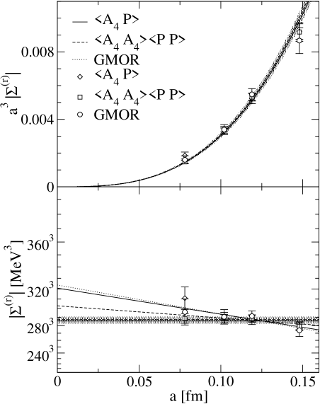
Figure 11: $a^{3}\,|\Sigma^{(r)}|$ and $|\Sigma^{(r)}|$ vs. $a$. In the legends we indicate the quantities used in the derivation of the condensate value. In the bottom plot we show a constant extrapolation (horizontal error bands) and compare it to a linear one.

So far we have restricted ourselves to the discussion of the largest physical volume results for only two lattice spacings, corresponding to $\beta=7.90$ and 8.15. In order to analyze the scaling behavior in the continuum limit we show in Fig. 11 the values for all lattice spacings (always for the largest volume) studied. Different physical lattice volumes are combined in this figure. As may be seen from the upper part of the plot, the leading $a^{3}$-dependence is suggestive.

In the lower part of the figure we exhibit the renormalized condensate by dividing out the expected leading $\mathcal{O}(a^{3})$ scale dependence. Since the Dirac action used obeys the GWC not exactly we cannot exclude linear corrections to perfect scaling. In GaGoHa03a these were found to be small for the hadron masses. For the condensate some of these corrections are already taken into account by the (independently determined) $Z$-factors in the determining equations.

For estimating the systematic error of the continuum extrapolation we therefore perform both, a constant fit (no scaling corrections) and a linear fit to the $a$-dependence. We do this for each type of derivation. The average of the resulting values for the constant fit is $|\Sigma^{(r)}|=(286(4)~{}\textrm{MeV})^{3}$; the linear fit leads to a larger value $|\Sigma^{(r)}|\approx(318(25)~{}\textrm{MeV})^{3}$. For the final value we give the result of the constant fit but quote the difference to the linear fit result as systematical error. Thus we find

$$|\Sigma^{(r)}|=(286(4)(32)~{}\textrm{MeV})^{3}\;.$$ (46)

This value is slightly larger, although still in the error limits of a determination from the overlap action BaBeGa05 and larger than the corresponding results in Ref. ChHs03 ; BiSh05 . Our numbers are in good agreement with calculations in the $\epsilon$-regime GiHeLa0304 ; FuHaOk05 . They also agree with a recent continuum extrapolation of the condensate based on the spectral distribution of the overlap operator WeWi05 .

IV.4 Pion decay constant

The pseudoscalar decay constants have been extracted from the asymptotic behavior of the pseudoscalar correlation functions according to (29) for pion and kaon, respectively. (See also DaHeSp05 for another method to determine $f_{\pi}$.)

In Fig. 13 we compare these results. When plotting them as functions of the respective pseudoscalar masses in Fig. 13, the data for pion and kaon essentially overlap each other and exhibit a universal functional behavior. We also show the error band of a quadratic extrapolation to the chiral limit.

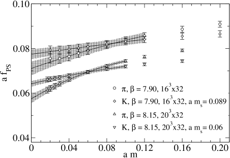
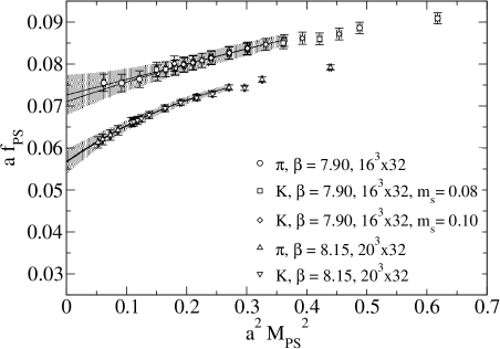
Figure 12: The dimensionless decay constants $a\,f_{\pi}$ and $a\,f_{K}$, determined with Eq. (29), vs. $a\,m$.

Figure 13: $a\,f_{\pi,K}$ vs. $(a\,M_{PS})^{2}$ with error bands for chiral extrapolations as discussed in the text. The fit includes only data in the indicated range.

For full QCD the chiral expansion of the pion decay constant should behave like CoGaLe01 :

$$f_{\pi}/f=1+\xi\,\bar{\ell}_{4}+\mathcal{O}(\xi^{2})\quad\textrm{with}\quad\xi=\left(\frac{M_{\pi}}{4\,\pi\,F_{\pi}}\right)^{2}\;.$$ (47)

The value $\bar{\ell}_{4}=-\ln(M_{\pi}^{2}/\Lambda^{2})$ depends on the intrinsic QCD scale $\Lambda$ and in CoGaLe01 it is suggested to use $\Lambda\approx 4\,\pi\,f_{\pi}$; in Ref. AnCaCo04 a value of $\bar{\ell}_{4}\approx 4.0\pm 0.6$ is quoted.

ChPT also relates the decay constant to the scalar form factor radius via

$$f_{\pi}/f=1+\frac{1}{6}\langle r^{2}\rangle_{s}M_{\pi}^{2}+\frac{13}{12}\xi+\mathcal{O}(\xi^{2})\;.$$ (48)

The relation holds for both, the pion and the kaon; this behavior is confirmed by our results in Fig. 13.

Eq. (48) may be translated to

$$\langle r^{2}\rangle_{s}=\frac{3}{8\,\pi^{2}\,f_{\pi}^{2}}\,\left(\bar{\ell}_{4}-\frac{13}{12}+\mathcal{O}(\xi)\right)\;.$$ (49)

The authors of Ref. AnCaCo04 quote an expected value of $f_{\pi}/f=1.072(4)$ and $\langle r^{2}\rangle_{s}=0.61(4)\,\textrm{fm}^{2}$.

In our quenched QCD case one expects correction terms with a logarithmic singularity in the valence quark mass $m$. As pointed out in Sh92 the leading order logarithmic term $m\,\log m$ of ChPT involves quark loops that are absent in the quenched case. There will be non-leading, e.g., logarithmic, terms, though. We therefore allow in addition to the linear term in the quark mass $m$ also a term $m^{2}\,\log m$ in the extrapolating fit (cf. the discussion in DoDrHo04 ). Actually, in the fit it makes no significant difference whether we take this term or just $m^{2}$.

When removing the leading scale dependent factors, thus changing to physical values, in Fig. 14 we find still non-negligible $a$-dependence away from the chiral limit. Note that the physical values of $f_{\pi}$ and $f_{K}$ have to be read off at the respective different values of $m_{\textrm{\scriptsize PS}}$.

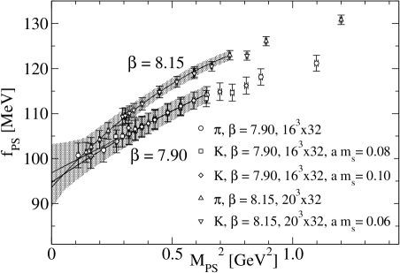
Figure 14: Chiral limit of $f_{\pi,K}$ vs. $M_{PS}^{2}$. Error bands for quadratic extrapolation.

Fig. 14 (neglecting possible quenching effects) may be analyzed according to the ChPT expansion (47). We see, however, that the slope near the chiral limit shows considerable $a$-dependence. Taking the slopes at face value we obtain values for $\langle r^{2}\rangle_{s}$ of 0.08 $\textrm{fm}^{2}$ and 0.13 $\textrm{fm}^{2}$, considerably smaller than expected for full QCD.

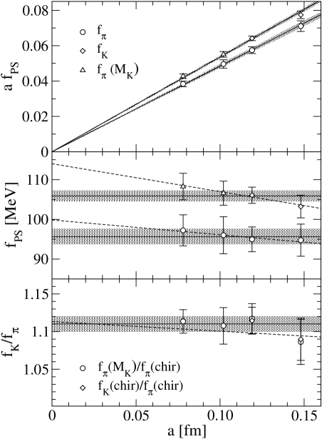
Figure 15: $a\,f_{\pi,K}$, $f_{\pi,K}$ and $f_{K}/f_{\pi}$ vs. $a$.

For a better study of the scale dependence we plot in Fig. 15 data for all lattice spacings, always for the largest volumes studied here. This plot combines different physical volumes. As can be seen in the upper part of the figure, the expected leading $a$-dependence is nicely exhibited. In the middle part of the figure we have removed the leading $a$-dependence.

As mentioned above in our discussion of the condensate, we expect the linear corrections to the leading scaling behavior to be small, but cannot exclude them, since the action is not an exact GW-operator. Like for the condensate we estimate the systematic error by fitting the data to a constant (no scaling violations) and a linear behavior in the lattice spacing and quote the difference as systematic error. The constant extrapolation for the pion gives $f_{\pi}=96(2)$ and the linear one gives $f_{\pi}=100(10)$. We therefore obtain as final continuum extrapolation

$$f_{\pi}=96(2)(4)\;\textrm{MeV}\;.$$ (50)

For the kaon we have results for non-degenerate quark masses only at two lattice spacings (same physical volume) and an extrapolation is thus underdetermined. At the other values of the lattice spacing studied we therefore compute values for $f_{PS}$ from the $f_{\pi}$-results at that mass $\overline{m}$, where at the pseudoscalar state for equal-mass quarks agrees with the kaon mass. This is the usual method when only one quark mass is considered and is justified from the universal behavior observed, e.g., in Fig. 13. The corresponding numbers are indicated by triangles in Fig. 15. Extrapolating in the same manner as discussed for the pion we end up with

$$f_{K}=106(1)(8)\;\textrm{MeV}\;.$$ (51)

We expect the leading corrections to scaling to cancel in the ratio $f_{K}/f_{\pi}$, plotted in the lower part of Fig. 15, and indeed the ratio is compatible with constant behavior. The continuum extrapolation along the lines discussed above gives the result

$$f_{K}/f_{\pi}=1.11(1)(2)\;.$$ (52)

Studies for the overlap action in quenched simulations have obtained similar results for $f_{\pi}$ DoDrHo04 ; GiHeLa0304 ; FuHaOk05 ; BiSh05 ; DuHo05 ; BaBeGa05 . The experimental values are $f_{\pi}=92.4(0.3)\;\textrm{MeV}$ and $f_{K}=113.0(1.3)\;\textrm{MeV}$ PDBook04 (taking into account the factor $\sqrt{2}$ in the definition).

V Conclusion

Within the Bern-Graz-Regensburg collaboration two Ginsparg-Wilson type Dirac operators (FP fermions and the so-called chirally improved Dirac operator) have been studied, both obeying the GWC to a good approximation. For the chirally improved Dirac operator we know the quark bilinear renormalization constants GaGoHu04 . This enables us to determine basic low energy constants for the light- and strange quark sector. All the results presented here are in the quenched approximation, i.e., without taking into account dynamical sea quarks. Due to the complicated and expensive form of the Ginsparg-Wilson type operators, a full QCD study still is a task for future work.

Since the chirally improved operator is substantially less expensive in computational means than the overlap operator, it was possible to work at several lattice spacings ranging from 0.15 fm down to 0.08 fm and with different lattice sizes. The results presented here are based mainly on simulations for lattice spacing 0.15 fm and 0.12 fm on lattices with a physical spatial extent of 2.4 fm. For an investigation of the scaling behavior and for studying finite size effects we also consider results from the other lattice parameter sets with different size and lattice constants. The data cover pion masses down to 330 MeV.

In the range of our simulation parameters we cannot reliably identify behavior specific for QChPT. Therefore the data have been extrapolated towards the chiral limit with the leading order ChPT expansion for full QCD. All physical values have been converted to the $\overline{\textrm{MS}}$-scheme (at scale 2 GeV). We end up with the following final (physical, renormalized) values:

$$\begin{array}[]{rccl}\textrm{Quark masses:}&\bar{m}&=&4.1(2.4)\;\textrm{MeV}\;,\\ &m_{s}&=&101(8)\;\textrm{MeV}\;,\\ \textrm{Condensate:}&\Sigma&=&-(286(4)(32)~{}\textrm{MeV})^{3}\;,\\ \textrm{Decay constants:}&f_{\pi}&=&96(2)(4)\;\textrm{MeV}\;,\\ &f_{K}&=&106(1)(8)\;\textrm{MeV}\;,\\ &f_{K}/f_{\pi}&=&1.11(1)(2)\;.\end{array}$$ (53)

Like many quenched results, these numbers are surprisingly close to the experimental values PDBook04 .

*

Appendix A Tables

Here we collect our main results for the meson and quark masses, for the condensate and the decay constants. All quantities are given as renormalized ones, i.e., including the renormalization factors converting them to the $\overline{\textrm{MS}}$-scheme at $\mu=2~{}\textrm{GeV}$.

Table 4: The pion and kaon masses computed from Eq. (26) on the $16^{3}\times 32$, $\beta=7.90$ lattice. As soon as the light quark mass exceed the (fixed) strange quark mass, the kaon becomes lighter than the pion.

$a\,m$	$a^{2}\,M_{\pi}^{2}$	$M_{\pi}^{2}[\textrm{GeV}^{2}]$	$M_{\pi}[\textrm{MeV}]$	$a^{2}\,M_{K}^{2}$	$M_{K}^{2}[\textrm{GeV}^{2}]$	$M_{K}[\textrm{MeV}]$
0.02	0.062(3)	0.110(5)	332(7)	0.163(2)	0.290(3)	538(3)
0.03	0.092(2)	0.163(4)	404(5)	0.178(2)	0.317(4)	563(3)
0.04	0.121(2)	0.216(4)	465(4)	0.194(2)	0.344(4)	586(4)
0.05	0.151(2)	0.269(4)	519(4)	0.209(2)	0.371(4)	609(4)
0.06	0.181(2)	0.322(4)	568(4)	0.224(3)	0.398(5)	631(4)
0.08	0.241(3)	0.429(5)	655(4)	0.254(3)	0.452(5)	672(4)
0.10	0.301(3)	0.536(6)	732(4)	0.284(3)	0.505(5)	711(4)
0.12	0.362(3)	0.644(6)	803(4)	0.314(3)	0.559(6)	747(4)
0.16	0.488(4)	0.868(7)	931(4)	0.375(3)	0.666(6)	816(4)
0.20	0.618(4)	1.098(7)	1048(3)	0.436(4)	0.775(7)	880(4)

Table 5: The pion and kaon masses computed from Eq. (26) on the $20^{3}\times 32$, $\beta=8.15$ lattice.

$a\,m$	$a^{2}\,M_{\pi}^{2}$	$M_{\pi}^{2}[\textrm{GeV}^{2}]$	$M_{\pi}[\textrm{MeV}]$	$a^{2}\,M_{K}^{2}$	$M_{K}^{2}[\textrm{GeV}^{2}]$	$M_{K}[\textrm{MeV}]$
0.017	0.052(1)	0.143(4)	378(5)	0.108(2)	0.295(5)	543(4)
0.02	0.060(1)	0.164(4)	405(4)	0.112(2)	0.305(5)	553(4)
0.025	0.073(1)	0.199(4)	447(4)	0.118(2)	0.323(4)	568(4)
0.03	0.086(1)	0.235(4)	484(4)	0.125(2)	0.341(4)	584(4)
0.04	0.112(1)	0.305(4)	552(4)	0.138(1)	0.376(4)	613(3)
0.06	0.164(1)	0.448(4)	669(3)	0.164(1)	0.448(4)	669(3)
0.08	0.217(1)	0.592(4)	769(2)	0.190(1)	0.519(4)	721(3)
0.10	0.271(1)	0.739(4)	860(2)	0.217(1)	0.592(4)	769(2)
0.12	0.326(1)	0.890(4)	943(2)	0.243(1)	0.664(4)	815(2)
0.16	0.439(2)	1.200(5)	1096(2)	0.297(1)	0.810(4)	900(2)

Table 6: The light quark condensate as derived from different observables (lattice size $16^{3}\times 32$, $\beta=7.90$). In the last line we give the extrapolation to the chiral limit as discussed in the text.

$a\,m$	$a^{3}\,|\Sigma_{\langle A_{4}P\rangle}|$	$a^{3}\,|\Sigma_{\textrm{\scriptsize GMOR}}|$	$a^{3}\,|\Sigma_{\langle PP\rangle\langle A_{4}A_{4}\rangle}|$	$\sqrt[3]{|\Sigma_{\langle A_{4}P\rangle}|}[\textrm{MeV}]$	$\sqrt[3]{|\Sigma_{\textrm{\scriptsize GMOR}}|}[\textrm{MeV}]$	$\sqrt[3]{|\Sigma_{\langle PP\rangle\langle A_{4}A_{4}\rangle}|}[\textrm{MeV}]$
0.02	0.0101(5)	0.0101(8)	0.0104(5)	289(5)	288(8)	291(4)
0.03	0.0102(5)	0.0097(7)	0.0102(5)	289(4)	284(7)	290(5)
0.04	0.0103(4)	0.0098(6)	0.0103(5)	290(4)	285(6)	290(4)
0.05	0.0105(4)	0.0101(6)	0.0104(5)	292(3)	288(6)	291(4)
0.06	0.0108(4)	0.0104(6)	0.0107(4)	295(3)	291(5)	293(4)
0.08	0.0113(4)	0.0111(6)	0.0113(4)	300(3)	297(5)	299(3)
0.10	0.0119(4)	0.0117(5)	0.0119(4)	305(3)	303(4)	304(3)
0.12	0.0125(4)	0.0123(5)	0.0125(4)	309(3)	308(4)	309(3)
0.16	0.0136(4)	0.0134(5)	0.0136(4)	318(3)	317(4)	319(3)
0.20	0.0146(4)	0.0144(5)	0.0146(4)	326(3)	324(4)	326(3)
chir.	0.0092(5)	0.0087(8)	0.0092(6)	279(5)	274(8)	279(6)

Table 7: The light quark condensate as derived from different observables (lattice size $20^{3}\times 32$, $\beta=8.15$).

$a\,m$	$a^{3}\,|\Sigma_{\langle A_{4}P\rangle}|$	$a^{3}\,|\Sigma_{\textrm{\scriptsize GMOR}}|$	$a^{3}\,|\Sigma_{\langle PP\rangle\langle A_{4}A_{4}\rangle}|$	$\sqrt[3]{|\Sigma_{\langle A_{4}P\rangle}|}[\textrm{MeV}]$	$\sqrt[3]{|\Sigma_{\textrm{\scriptsize GMOR}}|}[\textrm{MeV}]$	$\sqrt[3]{|\Sigma_{\langle PP\rangle\langle A_{4}A_{4}\rangle}|}[\textrm{MeV}]$
0.017	0.0058(4)	0.0061(3)	0.0059(2)	297(6)	302(5)	299(4)
0.02	0.0059(3)	0.0061(3)	0.0059(2)	298(6)	302(5)	299(4)
0.025	0.0060(3)	0.0061(3)	0.0060(2)	300(5)	302(5)	301(3)
0.03	0.0061(3)	0.0062(3)	0.0061(2)	302(4)	304(4)	302(3)
0.04	0.0063(2)	0.0065(2)	0.0063(2)	305(3)	308(4)	306(3)
0.06	0.0069(2)	0.0070(2)	0.0068(1)	314(3)	317(3)	314(2)
0.08	0.0074(2)	0.0076(1)	0.0074(1)	323(2)	324(2)	322(2)
0.10	0.0080(1)	0.0081(1)	0.0079(1)	330(2)	331(2)	329(1)
0.12	0.0085(1)	0.0085(1)	0.0084(1)	337(2)	338(2)	336(1)
0.16	0.0094(1)	0.0094(2)	0.0093(1)	349(2)	349(2)	348(1)
chir.	0.0052(3)	0.0055(3)	0.0053(2)	287(6)	291(6)	289(4)

Table 8: Pion and kaon decay constants (from Eq. (29)) for $16^{3}\times 32$, $\beta=7.90$ lattice. In the last line we give the extrapolation to the (semi-)chiral limit (where the light quark masses vanish) as it is discussed in the text.

$a\,m$	$a\,f_{\pi}/Z_{A}$	$a\,f_{\pi}$	$f_{\pi}[\textrm{MeV}]$	$a\,f_{K}/Z_{A}$	$a\,f_{K}$	$f_{K}[\textrm{MeV}]$
0.02	0.076(2)	0.076(2)	101(3)	0.080(2)	0.079(2)	106(2)
0.03	0.076(2)	0.075(2)	101(3)	0.080(2)	0.079(2)	106(2)
0.04	0.077(2)	0.076(2)	102(3)	0.080(2)	0.080(2)	106(2)
0.05	0.079(2)	0.078(2)	104(3)	0.081(2)	0.080(2)	107(2)
0.06	0.080(2)	0.079(2)	105(2)	0.082(2)	0.081(2)	108(2)
0.08	0.082(2)	0.082(2)	109(2)	0.083(2)	0.082(2)	109(2)
0.10	0.084(1)	0.084(1)	112(2)	0.084(1)	0.083(1)	111(2)
0.12	0.086(1)	0.086(1)	114(2)	0.085(1)	0.084(1)	112(2)
0.16	0.089(1)	0.089(1)	118(2)	0.086(1)	0.085(1)	114(2)
0.20	0.092(1)	0.091(1)	121(2)	0.087(1)	0.087(1)	115(2)
(semi-)chir.	0.072(3)	0.071(8)	95(4)	0.078(2)	0.077(2)	103(3)

Table 9: Pion and kaon decay constants (from Eq. (29)) for $20^{3}\times 32$, $\beta=8.15$ lattice.

$a\,m$	$a\,f_{\pi}/Z_{A}$	$a\,f_{\pi}$	$f_{\pi}[\textrm{MeV}]$	$a\,f_{K}/Z_{A}$	$a\,f_{K}$	$f_{K}[\textrm{MeV}]$
0.017	0.062(1)	0.061(1)	101(2)	0.067(1)	0.066(1)	109(2)
0.02	0.063(1)	0.062(1)	103(2)	0.067(1)	0.066(1)	110(2)
0.025	0.064(1)	0.063(1)	104(2)	0.067(1)	0.067(1)	110(2)
0.03	0.065(1)	0.064(1)	106(2)	0.0678(9)	0.0670(9)	111(1)
0.04	0.067(1)	0.0661(9)	109(2)	0.0686(8)	0.0679(8)	112(1)
0.06	0.0703(8)	0.0695(8)	115(1)	0.0703(8)	0.0695(8)	115(1)
0.08	0.0730(7)	0.0721(7)	119(1)	0.0716(7)	0.0708(7)	117(1)
0.10	0.0752(6)	0.0744(6)	123(1)	0.0728(7)	0.0720(7)	119(1)
0.12	0.0772(6)	0.0763(6)	126(1)	0.0737(7)	0.0729(7)	121(1)
0.16	0.0801(6)	0.0792(6)	131(1)	0.0752(6)	0.0743(6)	123(1)
(semi-)chir.	0.058(2)	0.058(2)	95(3)	0.065(1)	0.064(1)	106(2)

References

- (1) P. H. Ginsparg and K. G. Wilson, Phys. Rev. D 25, 2649 (1982).
- (2) M. Lüscher, Phys. Lett. B 428, 342 (1998).
- (3) R. Narayanan and H. Neuberger, Phys. Lett. B 302, 62 (1993).
- (4) R. Narayanan and H. Neuberger, Nucl. Phys. B 443, 305 (1995).
- (5) H. Neuberger, Phys. Lett. B 417, 141 (1998).
- (6) H. Neuberger, Phys. Lett. B 427, 353 (1998).
- (7) D. B. Kaplan, Phys. Lett. B 288, 342 (1992).
- (8) V. Furman and Y. Shamir, Nucl. Phys. B 439, 54 (1995).
- (9) P. Hasenfratz and F. Niedermayer, Nucl. Phys. B 414, 785 (1994).
- (10) C. Gattringer, Phys. Rev. D 63, 114501 (2001).
- (11) C. Gattringer, I. Hip, and C. B. Lang, Nucl. Phys. B 597, 451 (2001).
- (12) C. Gattringer et al., Nucl. Phys. B 677, 3 (2004).
- (13) L. Giusti, C. Hoelbling, and C. Rebbi, Phys. Rev. D 64, 114508 (2001); Err. ibid. 65, 079903 (2002).
- (14) L. Giusti, C. Hoelbling, and C. Rebbi, Nucl. Phys. B (Proc. Suppl.) 106, 739 (2002).
- (15) R. Babich et al., hep-lat/0509027.
- (16) L. Giusti, M. Lüscher, P. Weisz, and H. Wittig, JHEP 0311, 023 (2003).
- (17) T.-W. Chiu and T.-H. Hsieh, Nucl. Phys. B 673, 217 (2003).
- (18) L. Giusti, P. Hernandez, M. Laine, P. Weisz, and H. Wittig, JHEP 01, 003 (2004); JHEP 04, 013 (2004).
- (19) S. Dong et al., Phys. Rev. D 65, 054507 (2002).
- (20) T. Draper et al., Nucl. Phys. Proc. Suppl. 119, 239 (2003).
- (21) P. Hernandez, K. Jansen, and L. Lellouch, Phys. Lett. B 469, 198 (1999).
- (22) P. Hasenfratz, S. Hauswirth, T. Jörg, F. Niedermayer, and K. Holland, Nucl. Phys. B 643, 280 (2002).
- (23) J. Wennekers and H. Wittig, JHEP 05 059 (2005).
- (24) W. Bietenholz and S. Shcheredin, PoS (LAT2005) 138 (2005); ibid. 134 (2005).
- (25) S. Dürr and C. Hoelbling, hep-ph/0508085.
- (26) C. Gattringer et al., Nucl. Phys. B (Proc. Suppl.) 119, 796 (2003).
- (27) C. Gattringer, M. Göckeler, P. Huber, and C. B. Lang, Nucl. Phys. B 694, 179 (2004).
- (28) M. Lüscher and P. Weisz, Commun. Math. Phys. 97, 59 (1985).
- (29) G. Martinelli, C. Pittori, C. T. Sachrajda, M. Testa, and A. Vladikas, Nucl. Phys. B 445, 81 (1995).
- (30) M. Göckeler et al., Nucl. Phys. B 544, 699 (1999).
- (31) S. Eidelman et al., Phys. Lett. B 592, 1 (2004).
- (32) S. Weinberg, Physica A 96, 327 (1979).
- (33) J. Gasser and H. Leutwyler, Ann. Phys. 158, 142 (1984).
- (34) A. Hasenfratz and F. Knechtli, Phys. Rev. D 64, 034504 (2001).
- (35) C. Gattringer, R. Hoffmann, and S. Schaefer, Phys. Rev. D 65, 094503 (2002).
- (36) C. Hagen, Spectroscopy of baryons and exotic hadrons on the lattice, Diploma thesis, Univ. Regensburg (2005).
- (37) S. Güsken et al., Phys. Lett. B 227, 266 (1989).
- (38) C. Best et al., Phys. Rev. D 56, 2743 (1997).
- (39) T. Burch et al., Phys. Rev. D 70, 054502 (2004).
- (40) C. W. Bernard and M. F. L. Golterman, Phys. Rev. D 46, 853 (1992).
- (41) S. R. Sharpe, Phys. Rev. D 46, 3146 (1992).
- (42) C. W. Bernard and M. F. L. Golterman, Phys. Rev. D 49, 486 (1994).
- (43) S. R. Sharpe, Phys. Rev. D 56 (1997); Err. ibid. 62, 099901 (2000).
- (44) S. J. Dong et al., Phys. Rev. D 70, 034502 (2004).
- (45) T. Blum et al., Phys. Rev. D 69, 074502 (2004).
- (46) J. Heitger, R. Sommer, and H. Wittig, Nucl. Phys. B 588, 377 (2000).
- (47) M. Hofmayer, Hadronic properties of chirally improved Dirac operators, Diploma thesis, Univ. Graz (2004).
- (48) J. Gasser and H. Leutwyler, Phys. Lett. B 188, 477 (1987).
- (49) H. Fukaya, S. Hashimoto, and K. Ogawa, Prog. Theor. Phys. 114 451 (2005). hep-lat/0504018.
- (50) P.H. Damgaard, U.M. Heller, K. Splittorff, and B. Svetitsky, hep-lat/0508029.
- (51) G. Colangelo, J. Gasser, and H. Leutwyler, Nucl. Phys. B 603, 125 (2001).
- (52) B. Ananthanarayan, I. Caprini, G. Colangelo, J. Gasser, and H. Leutwyler, Phys. Lett. B 602, 218 (2004).