Nonperturbative $O(a)$ improvement of the Wilson quark action with the RG-improved gauge action using the Schrödinger functional method

Abstract

We perform a nonperturbative determination of the $O(a)$-improvement coefficient $c_{\rm SW}$ and the critical hopping parameter $\kappa_{c}$ for $N_{f}$=3, 2, 0 flavor QCD with the RG-improved gauge action using the Schrödinger functional method. In order to interpolate $c_{\rm SW}$ and $\kappa_{c}$ as a function of the bare coupling, a wide range of $\beta$ from the weak coupling region to the moderately strong coupling points used in large-scale simulations is studied. Corrections at finite lattice size of $O(a/L)$ turned out to be large for the RG-improved gauge action, and hence we make the determination at a size fixed in physical units using a modified improvement condition. This enables us to avoid $O(a)$ scaling violations which would remain in physical observables if $c_{\rm SW}$ determined for a fixed lattice size $L/a$ is used in numerical simulations.

I Introduction

Fully unquenched simulations of QCD with dynamical up, down and strange quarks have become feasible Ishikawa:2004nm thanks to the recent development of algorithms Kennedy:2004ae and computational facilities. However, it is still very demanding to control discretization errors below a few percent level in dynamical QCD simulations. Thus highly improved lattice actions are desirable to accelerate the approach to the continuum limit.

The on-shell improvement of the Wilson quark action through $O(a)$ requires only a single additional term, i.e. the Sheikholeslami-Wohlert (SW) term Sheikholeslami:1985ij . In Ref. Yamada:2004ja , we determined $c_{\rm SW}$ in three-flavor QCD for the plaquette gauge action, using the Schrödinger functional method SF ; NPimprovement ; NPcsw.Nf0.ALPHA ; NPcsw.Nf2.ALPHA . Applications of the resulting $O(a)$ improved Wilson-clover quark action in combination with the plaquette gauge action suffer from a serious problem, however, since it was found in Ref. Aoki:2004iq that this action combination exhibits an unphysical first-order phase transition at zero temperature in the strong coupling regime ($\beta\leq$ 5.0).

We also found in Ref. Aoki:2004iq that such a phase transition weakens, and possibly disappears, when the gauge action is improved. In this work, motivated by this observation, we extend the determination of $c_{\rm SW}$ for the case of the RG-improved action Iwasaki:1983ck for gluons for $N_{f}$=3, 2, 0 flavor QCD.

We explore a wide range of $\beta$ to work out the interpolation formula as a function of the bare coupling. The critical hopping parameter $\kappa_{c}$ in the $O(a)$-improved theory is also obtained.

In the Schrödinger functional method, $c_{\rm SW}$ is determined such that the axial Ward-Takahashi identity is satisfied for a given finite volume. Since the linear extent $L$ of a finite lattice provides an energy scale $1/L$, a determination of $c_{\rm SW}$ generally involves corrections of order $a/L$. We find that this correction is sizable for the RG improved gauge action. If the determination of $c_{\rm SW}$ is made for a fixed value of $L/a$, observables calculated in subsequent simulations using such $c_{\rm SW}$ would suffer from $O(a)$ scaling violations. To avoid this problem, we modify the standard improvement condition and determine $c_{\rm SW}$ at a fixed physical size $L$. Similar considerations have been made in the determinations of some other $O(a)$ improvement coefficients in Ref. Luscher:1996jn ; Guagnelli:2000jw .

This paper is organized as follows. In Sec.II, we briefly recall the Schrödinger functional method, mainly to fix notations. In Sec. III, corrections at finite lattice size of $O(a/L)$ that affect $c_{\rm SW}$ are discussed, and our modified method and one-loop calculations relevant for the subsequent analyses are given. Section IV is devoted to describing our numerical results, and Sec. V to systematic uncertainties in them. Our conclusions are given in Sec. VI. A preliminary report of this work has been made in Ref. Aoki:2002vh .

II Schrödinger functional method for the determination of $c_{\rm SW}$

We briefly introduce the setup of the Schrödinger functional (SF) method and the improvement condition developed in Refs. SF ; NPimprovement ; NPcsw.Nf0.ALPHA ; NPcsw.Nf2.ALPHA .

II.1 SF setup

Consider the SF defined on a four dimensional hypercubic lattice with a volume $L^{3}\times T$ and the cylindrical geometry, i.e., the periodic boundary condition is imposed in the spatial directions and the Dirichlet one in the temporal direction for both gauge and quark fields. At the temporal boundaries $x_{0}=0$ and $T$, the following conditions are imposed on the link variables and the quark fields: the spatial link variables on the boundaries are fixed to the diagonal, constant $SU(3)$ matrices given by

$$\left.U_{k}({\bf x},x_{0})\right|_{x_{0}\!=\!0}=\exp\left[aC_{k}\right],\ \ \ \left.U_{k}({\bf x},x_{0})\right|_{x_{0}\!=\!T}=\exp\left[aC_{k}^{\prime}\right],$$ (1)

$$C_{k}=\frac{i\pi}{6L_{k}}\left(\begin{array}[]{rrr}-1&0&0\\ 0&0&0\\ 0&0&1\end{array}\right),\ \ \ C_{k}^{\prime}=\frac{i\pi}{6L_{k}}\left(\begin{array}[]{rrr}-5&0&0\\ 0&2&0\\ 0&0&3\end{array}\right),$$ (8)

while all quark fields on the boundaries are set to zero.

We use the RG-improved gauge action Iwasaki:1983ck given by,

$$S_{g}=\frac{2}{g^{2}}\times\Big{[}~{}\sum_{x}~{}w^{P}_{\mu\nu}(x_{0})~{}{\rm Re~{}Tr}\left(1-P_{\mu,\nu}(x)\right)~{}+~{}\sum_{x}~{}w^{R}_{\mu\nu}(x_{0})~{}{\rm Re~{}Tr}\left(1-R^{(1\times 2)}_{\mu,\nu}(x)\right)\Big{]},$$ (9)

where $P_{\mu,\nu}(x)$ denotes a 1$\times$1 Wilson loop on the $\mu$-$\nu$ plane starting and ending at $x$, and $R^{(1\times 2)}_{\mu,\nu}(x)$ a 1$\times$2 rectangular loop with the side of length 2 in the $\nu$ direction. These terms are added up with proper weights, $w^{P}_{\mu\nu}(x_{0})$ and $w^{R}_{\mu\nu}(x_{0})$, respectively. In ordinary simulations with the periodic boundary condition in the temporal direction, the weights are given by $w^{P}_{\mu\nu}$=3.648 and $w^{R}_{\mu\nu}$=$-$0.331 independently of $x_{0}$. In the SF, these weights are modified. Among several possible choices, we select the choice B defined in Ref. Aoki:1998qd in this work,

$$w^{P}_{\mu\nu}(x_{0}) = \left\{\begin{array}[]{ll}\displaystyle\frac{1}{2}\times(3.648)&\mbox{at $t=0$ or $T$ and $\mu$, $\nu\neq$4}\\[8.61108pt] 3.648&\mbox{otherwise}\end{array}\right.,$$ (12)

$$w^{R}_{\mu\nu}(x_{0}) = \left\{\begin{array}[]{ll}0&\mbox{at $t=0$ or $T$ and $\mu$, $\nu\neq$4}\\[4.30554pt] \displaystyle\frac{3}{2}\times(-0.331)&\mbox{at $t=0$ or $T$ and $\mu$=4}\\[4.30554pt] -0.331&\mbox{otherwise}\end{array}\right..$$ (16)

The $O(a)$-improved Wilson quark action Sheikholeslami:1985ij is given by

$$S_{q} = \sum_{x,y}\bar{q}_{x}D_{xy}q_{y},$$ (17)

$$D_{xy} = \delta_{xy}-\kappa\sum_{\mu}\left\{\left(1-\gamma_{\mu}\right)U_{x,\mu}\delta_{x+\hat{\mu},y}+\left(1+\gamma_{\mu}\right)U_{x-\hat{\mu},\mu}^{\dagger}\delta_{x-\hat{\mu},y}\right\}+\frac{i}{2}\kappa\ c_{\rm SW}\sigma_{\mu\nu}F_{x,\mu\nu}\delta_{xy},$$ (18)

with the field strength tensor $F_{x,\mu\nu}$ defined by

$$F_{x,\mu\nu} = \frac{1}{8}\left\{\left(P_{\mu,\nu}(x)+P_{\nu,-\mu}(x)+P_{-\mu,-\nu}(x)+P_{-\nu,\mu}(x)\right)-\left(\mbox{h.c.}\right)\right\},$$ (19)

and $\sigma_{\mu\nu}=(i/2)\left[\gamma_{\mu},\gamma_{\nu}\right]$. The last term in Eq. (18) is the only counter term to get rid of $O(a)$ errors present for on-shell quantities on the lattice. At tree level, $c_{\rm SW}$=1. For the $O(a)$-improvement of the SF, we need to add extra terms made of the gauge and quark fields at boundaries to the lattice action. However, since these counter terms affect the PCAC relation used in the following calculations only at $O(a^{2})$ or higher, they are not necessary for the determination of $c_{\rm SW}$.

II.2 PCAC relation

We determine $c_{\rm SW}$ by imposing the PCAC relation

$$\frac{1}{2}\left(\partial_{\mu}+\partial_{\mu}^{*}\right)A_{{\rm imp},\mu}^{a}=2m_{q}P^{a},$$ (20)

up to $O(a^{2})$ corrections. The pseudo-scalar density operator, axial vector current and its $O(a)$-improved version are given by

$$P^{a} = \bar{\psi}\gamma_{5}\tau^{a}\psi,$$ (21)

$$A_{\mu}^{a} = \bar{\psi}\gamma_{\mu}\gamma_{5}\tau^{a}\psi,$$ (22)

$$A_{{\rm imp},\mu}^{a} = A_{\mu}^{a}+c_{A}\frac{1}{2}\left(\partial_{\mu}+\partial_{\mu}^{*}\right)P^{a},$$ (23)

where $\partial_{\mu}$ and $\partial_{\mu}^{*}$ are the forward and backward lattice derivatives, and $\tau^{a}$ denotes the generator of $SU(N_{f})$ flavor symmetry acting on the flavor indices of the quark fields $\bar{\psi}$ and $\psi$.

We measure two correlation functions,

$$f_{A}(x_{0}) = -\frac{1}{N_{f}^{2}-1}\langle A_{0}^{a}(x){\mathcal{O}}^{a}\rangle,$$ (24)

$$f_{P}(x_{0}) = -\frac{1}{N_{f}^{2}-1}\langle P^{a}(x){\mathcal{O}}^{a}\rangle,$$ (25)

where $x=(x_{0},{\bf x})$, and $\langle\cdots\rangle$ represents the expectation value after taking trace over color and spinor indices and summing over spatial coordinate $\bf x$. The source operator is given by

$${\mathcal{O}}^{a} = a^{6}\sum_{\bf y,z}\bar{\zeta}({\bf y})\gamma_{5}\tau^{a}\zeta({\bf z}),$$ (26)

$$\zeta({\bf x}) = \frac{\delta}{\delta\bar{\rho}({\bf x})},\ \ \ \bar{\zeta}({\bf x})=\frac{\delta}{\delta\rho({\bf x})},$$ (27)

where $\rho({\bf x})$ is the quark field at $x_{0}\!=\!0$ and is set to zero in the calculation of $f_{A}$ and $f_{P}$. The bare PCAC quark mass is then calculated using $f_{A}$ and $f_{P}$ through the PCAC relation Eq. (20) as

$$m(x_{0}) = r(x_{0})+c_{A}s(x_{0})$$ (28)

$$r(x_{0}) = \frac{1}{4}\left(\partial_{0}+\partial_{0}^{*}\right)f_{A}(x_{0})/f_{P}(x_{0})$$ (29)

$$s(x_{0}) = \frac{1}{2}a\,\partial_{0}\partial_{0}^{*}f_{P}(x_{0})/f_{P}(x_{0}).$$ (30)

Using the source operator on the other boundary

$${\mathcal{O}}^{\prime,a} = a^{6}\sum_{\bf y,z}\bar{\zeta}^{\prime}({\bf y})\gamma_{5}\tau^{a}\zeta^{\prime}({\bf z}),$$ (31)

where $\zeta^{\prime}$ is the boundary field at $x_{0}\!=\!T$, we can calculate another set of quantities $m^{\prime}(x_{0})$, $r^{\prime}(x_{0})$ and $s^{\prime}(x_{0})$ from the correlation functions defined by

$$f_{A}^{\prime}(T-x_{0}) = +\frac{1}{N_{f}^{2}-1}\langle A_{0}^{a}(x){\mathcal{O}}^{\prime,a}\rangle,$$ (32)

$$f_{P}^{\prime}(T-x_{0}) = -\frac{1}{N_{f}^{2}-1}\langle P^{a}(x){\mathcal{O}}^{\prime,a}\rangle,$$ (33)

A naive improvement condition would be $m(x_{0})\!=\!m^{\prime}(x_{0})$. However, this condition requires a nonperturbative tuning of $c_{A}$ as well as of $c_{\rm SW}$. To eliminate $c_{A}$ from the determination, it was proposed in Ref. NPcsw.Nf0.ALPHA to use an alternative definition of the quark mass given by

$$M(x_{0},y_{0}) = m(x_{0})-\frac{m(y_{0})-m^{\prime}(y_{0})}{s(y_{0})-s^{\prime}(y_{0})}s(x_{0}),$$ (34)

$$M^{\prime}(x_{0},y_{0}) = m^{\prime}(x_{0})-\frac{m^{\prime}(y_{0})-m(y_{0})}{s^{\prime}(y_{0})-s(y_{0})}s^{\prime}(x_{0}).$$ (35)

with which $c_{\rm SW}$ is obtained at the point where the mass difference

$$\Delta M(x_{0},y_{0})=M(x_{0},y_{0})-M^{\prime}(x_{0},y_{0})$$ (36)

vanishes. In principle, we can take an arbitrary choice for $(x_{0},y_{0})$, since different choices result only in $O(a^{2})$ differences in physical observables. We follow the ALPHA Collaboration and use $(x_{0},y_{0})\!=\!(3T/4,T/4)$ for $\Delta M$, and $(T/2,T/4)$ for $M$. In the following, $M$ and $\Delta M$ without arguments denote $M(T/2,T/4)$ and $\Delta M(3T/4,T/4)$, respectively.

In previous studies, $c_{\rm SW}$ has been determined through the conditions

$$\left\{\begin{array}[]{lll}M(g^{2}_{0},L/a)&=&0,\\ \Delta M(g^{2}_{0},L/a)&=&\Delta M(0,L/a),\end{array}\right.$$ (39)

at a given $g^{2}_{0}$ and $L/a$. $\Delta M(0,L/a)$ on the right hand side, which is the tree-level value of $\Delta M(g^{2}_{0},L/a)$ at the massless point, is necessary in order that the resulting $c_{\rm SW}$ reproduces its tree-level value ($c_{\rm SW}$=1) in the weak coupling limit. In the next section, we address the issue of corrections at finite lattice size, and propose a new condition to avoid the problem.

III corrections at finite lattice size and modified improvement conditions

III.1 corrections at finite lattice size

In the standard approach, we first calculate $M(g^{2}_{0},L/a)$ and $\Delta M(g^{2}_{0},L/a)$ for a set of values of $c_{\rm SW}$ and $\kappa$. The results are fitted as a function of $c_{\rm SW}$ and $\kappa$ to find $c_{\rm SW}(g^{2}_{0},L/a)$ and $\kappa_{c}(g^{2}_{0},L/a)$ satisfying Eq. (39) at a given value of $g^{2}_{0}$ and $L/a$. The asymptotic $a$ dependence of $c_{\rm SW}(g^{2}_{0},L/a)$ and $\kappa_{c}(g^{2}_{0},L/a)$ obtained in such a way is expected to be

$$c_{\rm SW}(g^{2}_{0},L/a) = c_{\rm SW}(g^{2}_{0},\infty)+c_{L}\cdot(a/L)+c_{\Lambda}\cdot(a\Lambda_{\rm QCD})+O((a/L)^{2},(a^{2}\Lambda_{\rm QCD}/L),(a\Lambda_{\rm QCD})^{2}),$$ (40)

$$\kappa_{c}(g^{2}_{0},L/a) = \kappa_{c}(g^{2}_{0},\infty)+k_{L}\cdot(a/L)+k_{\Lambda}\cdot(a\Lambda_{\rm QCD})+O((a/L)^{2},(a^{2}\Lambda_{\rm QCD}/L),(a\Lambda_{\rm QCD})^{2}),$$ (41)

where $c_{L}$, $c_{\Lambda}$, $k_{L}$ and $k_{\Lambda}$ are unknown coefficients. (In practice, a logarithmic dependence on $a/L$ also appears, but it does not alter the following discussion, and hence not written explicitly.)

Consider an on-shell physical quantity $Q$, and let $Q^{\rm latt}(a)$ be the value obtained on a lattice with lattice spacing $a$ using the SW quark action with a choice of the improvement coefficient $c_{\rm SW}^{\rm sim}$. We expect the discrepancy between $Q$ and $Q^{\rm latt}(a)$ in the measured value to be

$$Q-Q^{\rm latt}(a)=\ q\cdot\left(c_{\rm SW}^{\rm sim}-c_{\rm SW}(g^{2}_{0},\infty)\right)\cdot(a\Lambda_{\rm QCD})+O(a^{2}\Lambda_{\rm QCD}^{2}),$$ (42)

where $q$ is an unknown constant assumed to be $O(1)$. Hence, if one uses $c_{\rm SW}^{\rm sim}=c_{\rm SW}(g^{2}_{0},\infty)$ in the simulation, the $O(a)$ error is absent, while if one uses $c_{\rm SW}(g^{2}_{0},L/a)$ in Eq. (40), the above expression results in

$$Q-Q^{\rm latt}(a)=q\cdot c_{L}\cdot(a/L)\cdot(a\Lambda_{\rm QCD})+O(a^{2}\Lambda_{\rm QCD}^{2})+O(a\Lambda_{\rm QCD}(a/L)^{2}).$$ (43)

While the scaling violation appears to start from $O(a^{2})$, it is actually linear in the lattice spacing if one determines $c_{\rm SW}(g^{2}_{0},L/a)$ with a fixed value of $a/L$. Indeed, previous studies determining $c_{\rm SW}$ have used certain fixed values of $L/a$, e.g. 8, independently of $\beta$.

In Ref. Yamada:2004ja , we studied the magnitude of the corrections at finite lattice size in $c_{\rm SW}$ for the plaquette gauge action. The coefficient $c_{L}$ defined in Eq. (40) was evaluated in one-loop perturbation theory in the same SF setup, and it was found that the effect on $c_{\rm SW}$ does not exceed 3% when $L/a$=8 for $\beta\geq 5.2$. We have repeated the same perturbative analysis with the RG-improved action, and observed a sizable effect of about 15% at $\beta$=1.9, around which large-scale simulations are carried out. This enhancement of the one-loop correction for the RG improved action is mainly due to the larger value of the bare coupling compared to that for the plaquette gauge action for realizing the same value of the lattice spacing.

III.2 modified improvement condition

We propose to resolve the problem due to the sizable corrections explained above by introducing a fixed physical length $L^{*}$, and determining $c_{\rm SW}$ at the fixed physical volume ${L^{*}}^{3}\times T^{*}$ ($T^{*}=2L^{*}$). If one uses $c_{\rm SW}$ thus determined, $L$ in (43) is replaced by $L^{*}$ and scaling violations are $O(a^{2})$.

The actual procedure we use runs as follows. Instead of Eq. (39), we impose a modified improvement condition given by

$$\left\{\begin{array}[]{rrr}M(g^{2}_{0},L/a)&=&0,\\ \Delta M(g^{2}_{0},L/a)&=&0,\end{array}\right.$$ (46)

to calculate $c_{\rm SW}(g^{2}_{0},L/a)$ and $\kappa_{c}(g^{2}_{0},L/a)$. The results are converted to $c_{\rm SW}(g^{2}_{0},L^{*}/a)$ and $\kappa_{c}(g^{2}_{0},L^{*}/a)$. To do so, we must know the value of $L^{*}/a$ or $1/a$ at that value of $g^{2}_{0}$, which we obtain through the two-loop $\beta$ function,

$$a\Lambda_{L} = \exp\left(-\frac{1}{2b_{0}g_{0}^{2}}\right)(b_{0}g_{0}^{2})^{-b_{1}/2b_{0}^{2}},$$ (47)

$$b_{0} = \frac{1}{(4\pi)^{2}}\left(\frac{11}{3}N_{c}-\frac{2}{3}N_{f}\right),$$ (48)

$$b_{1} = \frac{1}{(4\pi)^{4}}\left(\frac{34}{3}N_{c}^{2}-N_{f}\left(\frac{13}{3}N_{c}-\frac{1}{N_{c}}\right)\right).$$ (49)

The transformation from $c_{\rm SW}(g^{2}_{0},L/a)$ and $\kappa_{c}(g^{2}_{0},L/a)$ to those at $L^{*}/a$ are made through

$$c_{\rm SW}(g^{2}_{0},L^{*}/a) = c_{\rm SW}(g^{2}_{0},L/a)+\delta c_{\rm SW}(g^{2}_{0},L/a;L^{*}/a),$$ (50)

$$\kappa_{c}(g^{2}_{0},L^{*}/a) = \kappa_{c}(g^{2}_{0},L/a)+\delta\kappa_{c}(g^{2}_{0},L/a;L^{*}/a),$$ (51)

where

$$\delta c_{\rm SW}(g^{2}_{0},L/a;L^{*}/a) = -c_{\rm SW}^{\mathrm{PT}}(g^{2}_{0},L/a)+c_{\rm SW}^{\mathrm{PT}}(g^{2}_{0},L^{*}/a),$$ (52)

$$\delta\kappa_{c}(g^{2}_{0},L/a;L^{*}/a) = -\kappa_{c}^{\mathrm{PT}}(g^{2}_{0},L/a)+\kappa_{c}^{\mathrm{PT}}(g^{2}_{0},L^{*}/a),$$ (53)

and $c_{\rm SW}^{\rm PT}(g^{2}_{0},L/a)$ and $\kappa_{c}^{\rm PT}(g^{2}_{0},L/a)$ are calculated at the one-loop level for the same SF setup at the given value of $L/a$.

It turned out that the tree and the one-loop coefficients for $c_{\rm SW}$ and $\kappa_{c}$ have a significant $a/L$ dependence. To describe this dependence precisely we fit them to a Pade or a polynomial-like function of $a/L$ as

$$c_{\rm SW}^{(0)}(L/a) = \frac{1+a_{1}\,(a/L)+a_{2}\,(a/L)^{2}+a_{3}\,(a/L)^{3}}{1+b_{1}\,(a/L)},$$ (54)

$$c_{\rm SW}^{(1)}(L/a) = 0.113+(c_{1}-d_{1}\ln(L/a))\,(a/L)+(c_{2}-d_{2}\ln(L/a))\,(a/L)^{2},$$ (55)

$$\kappa_{c}^{(0)}(L/a) = \frac{1}{8}+k_{1}\,(a/L)+k_{2}\,(a/L)^{2}+k_{3}\,(a/L)^{3}+k_{4}\,(a/L)^{4},$$ (56)

$$\kappa_{c}^{(1)}(L/a) = 0.002760894+(l_{1}-m_{1}\ln(L/a))\,(a/L)+(l_{2}-m_{2}\ln(L/a))\,(a/L)^{2}.$$ (57)

The coefficients are given in Table 1. We note that the one-loop coefficients have an $N_{f}$ dependence due to the tadpole diagram, although it vanishes in the large volume limit.

In our actual determination, we define $L^{*}$ by $L^{*}/a=6$ at $\beta=1.9$, $L^{*}/a=6$ at $\beta=2.0$ and $L^{*}/a=6$ at $\beta=2.6$ for $N_{f}$=3, 2, 0 flavor QCD, respectively. In Table 2–4 numerical values of $\beta=6/g^{2}_{0}$, $L/a$ and $L^{*}/a$ in our simulations for $N_{f}$=3, 2, and 0 cases are summarized. In these tables, we also show the numerical values of $\delta c_{\rm SW}(g^{2}_{0},L/a;L^{*}/a)$ and $\delta\kappa_{c}(g^{2}_{0},L/a;L^{*}/a)$. For large values of $\beta$, the perturbative corrections are small and hence reliable. On the other hand, if $L/a$ are close to $L^{*}/a$, the corrections needed for the conversion from $L$ to $L^{*}$ should again be small. Since we fix $L^{*}$ at strong coupling, the corrections, Eqs. (52) and (53), are small at both ends of our range of $\beta$ as one can see in the Tables.

IV Numerical simulations

IV.1 parameters and algorithm

The numerical simulations are performed with $N_{f}$=3, 2 and 0 degenerate dynamical quarks on a $(L/a)^{3}\times 2(L/a)$ ($L/a$= 8 or 6) lattice for a wide range of $\beta$. The simulation parameters are summarized in Tabs. 2–4 for $N_{f}$=3, 2, 0, respectively.

We employ the symmetric even-odd preconditioning introduced in Refs. Even-Odd ; PHMC.JLQCD for the quark matrix $D$. Calculation of $D^{-1}$ is made with the BiCGStab algorithm with the tolerance parameter $||R_{i}||/||B||\!<\!10^{-14}$, where $R_{i}=DX_{i}-B$ is the residual vector and $X_{i}$ is an estimate for the solution $X$ in the $i$-th BiCGStab iteration.

We adopt the standard HMC algorithm HMC for the $N_{f}$=2 and 0 flavor cases. For the three-flavor case, the polynomial HMC (PHMC) algorithm PHMC ; PHMC.JLQCD is applied to describe the third flavor, employing the Chebyshev polynomial $P[D]$ to approximate $D^{-1}$. In order to make the PHMC algorithm exact, the correction factor $P_{\rm corr}={\rm det}[W[D]]$ with $W[D]\!=\!P[D]D$ is taken into account by the noisy Metropolis method NoisyMetroP . The square root of $W[D]$, which is required in the Metropolis test, is evaluated with an accuracy of $10^{-14}$ using a Taylor expansion of $W[D]$ PHMC.JLQCD . The order of the polynomial $N_{\rm poly}$ is chosen so that an acceptance rate of about 70% or higher is achieved for the Metropolis test.

In the calculations of $aM$ and $a\Delta M$, $f_{X}$ and $f_{X}^{\prime}$ ($X$=$A$ or $P$) are first evaluated at every trajectory, and they are combined to produce $aM$ and $a\Delta M$. The bin size dependence of the jackknife error of $aM$ is investigated in the range $N_{\rm bin}\!=\!1$ – $N_{\rm traj}/20$. We adopt $N_{\rm bin}$ giving the maximum error in this range in the error analyses in the following.

IV.2 results

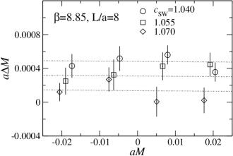
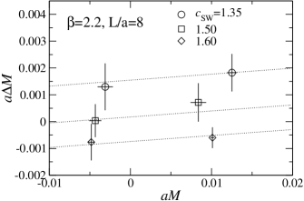
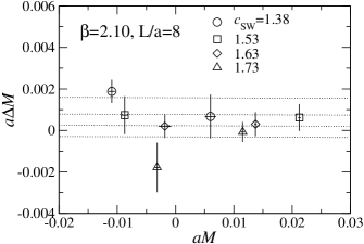
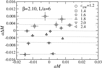
The trial values of $c_{\rm SW}$ and $\kappa$ at which simulations are made are summarized in Tables. LABEL:tab:Nf3MandDM–LABEL:tab:Nf0MandDM for $N_{f}$=3, 2, and 0, respectively, together with the results for $aM$ and $a\Delta M$ and the number of trajectories accumulated. In order to obtain $c_{\rm SW}(g^{2}_{0},L/a)$ and $\kappa_{c}(g^{2}_{0},L/a)$ satisfying Eq. (46) at each $\beta$, we make fits of those data using the functional forms,

$$aM = a_{M}+\frac{b_{M}^{(1)}}{\kappa}+\frac{b_{M}^{(2)}}{\kappa^{2}}+c_{M}^{(1)}\,c_{\rm SW}+c_{M}^{(2)}\,{c_{\rm SW}}^{2}+\frac{d_{M}}{\kappa}\,c_{\rm SW},$$ (58)

$$a\Delta M = a_{\Delta M}+\frac{b_{\Delta M}^{(1)}}{\kappa}+\frac{b_{\Delta M}^{(2)}}{\kappa^{2}}+c_{\Delta M}^{(1)}\,c_{\rm SW}+c_{\Delta M}^{(2)}\,c_{\rm SW}^{2}+\frac{d_{\Delta M}}{\kappa}\,c_{\rm SW}.$$ (59)

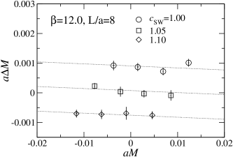
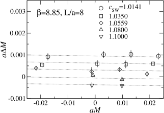
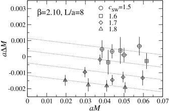
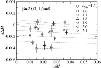
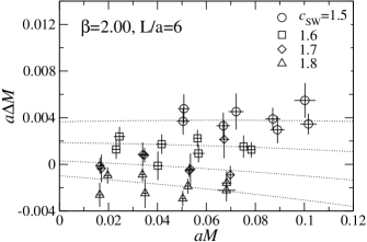
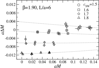
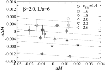
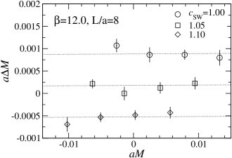
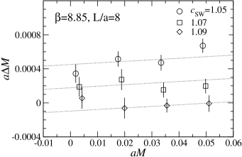
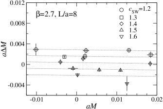
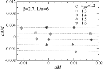
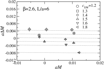
The results for $c_{\rm SW}(g^{2}_{0},L/a)$ and $\kappa_{c}(g^{2}_{0},L/a)$ obtained with the fits, and the adopted functional form are tabulated in Tabs. 8–10. The details of the fit procedure are as follows. In Figs. 1–3 we plot data on the $(aM,a\Delta M)$ plane for $N_{f}$=3, 2, 0, respectively. For those data for which the origin $(0,0)$ is contained in or close to the data region, we make a fit leaving only the constant and linear terms in Eqs. (58) and (59). This applies to all cases except for the three-flavor simulations at $\beta\leq$ 2.2, and the dotted lines in the figures show the fit results.

In the three-flavor simulations at $\beta\leq$ 2.2, the region of negative $aM$ is not covered, and the origin is missed by the data. This happens because the PHMC algorithm tends to fail at vanishing or negative PCAC quark masses at low $\beta$ due to large quantum fluctuations. Thus, at $\beta\leq$ 2.2, we are forced to extrapolate the data. In the extrapolation, three functional forms are examined: (i) linear, (ii) quadratic without the cross terms, and (iii) quadratic with the cross terms. At $\beta$=2.20 and 2.10, a linear function well fits the data, and we take this in the following analysis. The data at $\beta$=2.00 and 1.90 require the quadratic term, but it turns out that including the cross terms does not reduce $\chi^{2}$/dof significantly from that without the cross terms, and leads to $c_{\rm SW}(g^{2}_{0},L/a)$ and $\kappa_{c}(g^{2}_{0},L/a)$ consistent within one standard deviation. Thus, we adopt the quadratic function without the cross terms at these $\beta$, and $d_{M}$ and $d_{\Delta M}$ are always set to zero throughout this analysis.

Next, $c_{\rm SW}(g^{2}_{0},L/a)$ and $\kappa_{c}(g^{2}_{0},L/a)$ are transformed into those for the desired lattice volume, $(L^{*}/a)^{3}\times 2(L^{*}/a)$, along the line presented in Sec. III.2. Using Eqs. (50), (51) and the $\delta c_{\rm SW}$ and $\delta\kappa_{c}$ given in Tables 2–4, we obtain $c_{\rm SW}(g^{2}_{0},L^{*}/a)$ and $\kappa_{c}(g^{2}_{0},L^{*}/a)$ shown in Tables 11– 13. Notice that in Table 11 there are three results for $\beta$=2.0. The first and second one are obtained by transforming the data with $8^{3}\times 16$ and $6^{3}\times 12$ to those for $L^{*}/a\sim$6.805, respectively, and the third one is obtained by simply interpolating the two raw values at $L/a=8$ and $6$ in Table 8 to $L^{*}/a\sim$6.805, for which the corrections at finite lattice size are essentially corrected nonperturbatively. The two raw values, 1.670(56) at $L/a=8$ and 1.632(45) at $L/a=6$, are very close to each other and consistent within the error, and hence the linear interpolation to $L^{*}/a\sim 6.805$ is more reliable than the perturbative procedure. Similar observations are made at the second smallest $\beta$ in each $N_{f}$ flavor simulation, namely at $\beta$=2.10 for $N_{f}=2$ and at $\beta$=2.70 for $N_{f}=0$. Thus, at these $\beta$ the result interpolated to $L^{*}/a$ is adopted as our final result, and used in the following analysis. At the same time, it is worth noting that in all three cases the one-loop corrections have the right sign, which indicates that the one-loop correction dominates over higher loop corrections. Furthermore, the discrepancy between the results corrected perturbatively and nonperturbatively is found to be 5%, 3% and less than 1% for the $N_{f}$=3, 2 and 0 cases, respectively, while the size of one-loop correction itself at these $\beta$ is 6–7%, 5% and 2–3%. From this observation, we expect that the size of the one-loop correction gives a conservative estimate for the unknown higher loop corrections for all $\beta$.

IV.3 interpolation formula

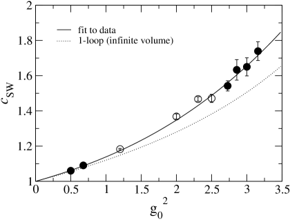
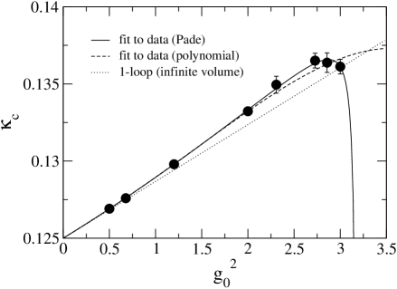
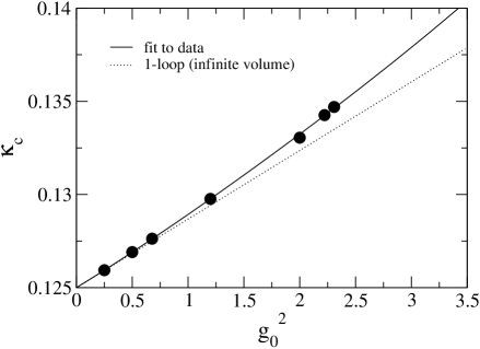
Our final results for $c_{\rm SW}(g^{2}_{0},L^{*})$ as a function of $g^{2}_{0}$ are shown in Fig. 4 for $N_{f}=3,2,0$ flavor QCD. When we interpolate $c_{\rm SW}$, not all available data are used in the fit. As mentioned in Sec. III.2, the corrections at finite lattice size estimated perturbatively is small only around the high and low ends of $\beta$ due to our choice of $L^{*}$, while in the middle range corrections may be significant. Therefore, we use data only if the correction is less than 5%. In the three flavor case, the data at $\beta$=12.0, 8.85, 2.2, 2.1, 2.0, 1.9 are employed. As a consequence, we obtain the followings interpolation formula,

$$c_{\rm SW}(g^{2}_{0},L^{*}) = 1+0.113\ g^{2}_{0}+0.0209(72)\ (g^{2}_{0})^{2}+0.0047(27)\ (g^{2}_{0})^{3},\ \ \ \ (\chi^{2}/{\rm dof}=0.58).$$ (60)

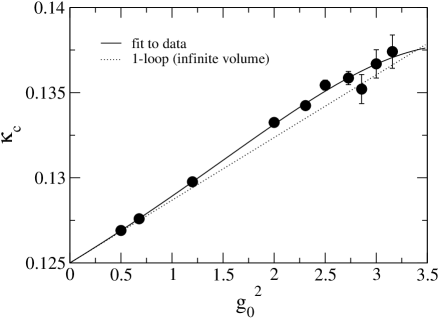
For $\kappa_{c}$ shown in Fig. 5, the corrections are smaller than 5% for all value of $\beta$. Including all data in the fit we obtain

$$\kappa_{c}(g^{2}_{0},L^{*}) = 1/8+0.003681192\ g^{2}_{0}+0.000211(43)\ (g^{2}_{0})^{2}$$ (61)

$$\ \ \ \ \ \ +0.000067(66)\ (g^{2}_{0})^{3}-0.000038(21)\ (g^{2}_{0})^{4}.\ \ \ \ (\chi^{2}/{\rm dof}=1.1)$$

When performing the above fits, the tree and one-loop coefficients are fixed to the perturbative values at infinite volume. This is justified since, as seen in Table 2, $L^{*}/a$ grows very rapidly with $\beta$, and hence $a/L^{*}$ corrections in Eqs. (54)–(57) are all negligibly small near the continuum limit. We also note that the tree and one-loop coefficients in the infinite volume limit do not depend on $N_{f}$, and hence the same values are used in the analysis for the $N_{f}$= 2 and 0 cases given below.

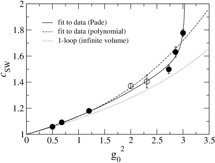
The interpolation formula for $c_{\rm SW}$ in two-flavor QCD is calculated in the same fashion as in the three-flavor case. In this case, the sizes of the correction at finite lattice size are acceptable ($\leq$ 5%) at $\beta$=12.0, 8.85, 5,0, 2.2, 2.1, 2.0. We first try a polynomial form as before, and obtain

$$c_{\rm SW}(g^{2}_{0},L^{*}) = 1+0.113\,g^{2}_{0}+0.0158(63)\,(g^{2}_{0})^{2}+0.0088(24)\,(g^{2}_{0})^{3},\ \ \ (\chi^{2}/{\rm dof}=4.68),$$ (62)

which is denoted by a dashed line in Fig. 4. A sharp rise of the data points near $g^{2}_{0}$=3.0 is not described well by this polynomial form, while in the three-flavor case the polynomial worked well over the whole range of $\beta$ we studied. An alternative is a Pade function, with which we obtain

$$c_{\rm SW}(g^{2}_{0},L^{*}) = \frac{1-0.212(9)\,g^{2}_{0}-0.0108(38)\,(g^{2}_{0})^{2}-0.0083(19)\,(g^{2}_{0})^{3}}{1-0.325(9)\,g^{2}_{0}},\ \ \ (\chi^{2}/{\rm dof}=2.11),$$ (63)

This fit, denoted by solid line in the middle panel of Fig. 4, interpolates our data very well. Since this formula has a pole at $g^{2}_{0}$=3.08(8), its use is restricted to $g^{2}_{0}\hbox to0.0pt{\raise-4.0pt\hbox{$\sim$}\hss}\raise 3.0pt\hbox{$<$}$3.0. For $\kappa_{c}$, we use all available data to obtain

$$\kappa_{c}(g^{2}_{0},L^{*}) = 1/8+0.003681192\,g^{2}_{0}+0.000227(58)\,(g^{2}_{0})^{2}$$ (64)

$$\ \ \ \ \ \ +0.000093(84)\,(g^{2}_{0})^{3}-0.000049(24)\,(g^{2}_{0})^{4},\ \ \ (\chi^{2}/{\rm dof}=0.98),$$

for a polynomial, and

$$\kappa_{c}(g^{2}_{0},L^{*}) = \frac{1/8-0.0356(23)\,g^{2}_{0}-0.00089(8)\,(g^{2}_{0})^{2}-0.00009(6)\,(g^{2}_{0})^{3}}{1-0.314(18)\,g^{2}_{0}},\ \ \ (\chi^{2}/{\rm dof}=0.35),$$ (65)

for a Pade function. These results appear in the middle panel of Fig. 5 as dashed and solid line, respectively. It is interesting that the pole positions for $c_{\rm SW}$ and $\kappa_{c}$ are consistent with each other. This seems to indicate that above $g^{2}_{0}\sim$3.0 the Wilson quark action cannot be improved in this fashion consistently for the $N_{f}$=2 case. All in all the Pade fits provide a more satisfactory interpolation of the $N_{f}$=2 data, and we take them as the main result for the $N_{f}$=2 case. We have also applied a Pade function for $c_{\rm SW}$ in the $N_{f}$=3 case. However, in this case the resulting fit lies on top of that for a polynomial over the range of $\beta$ we used, and the position of pole can be determined only poorly. Hence there seems no reason to favor the Pade fit over the polynomial for interpolating the data. The difference between the $N_{f}$=2 and 3 cases probably arise from the fact, empirically known, that the $N_{f}$=2 lattice is coarser than the $N_{f}$=3 lattice at the same value of $g^{2}_{0}$. Indeed, a sharp rise of improvement coefficients was previously seen for the plaquette gauge action toward coarse lattices NPcsw.Nf0.ALPHA ; NPcsw.Nf2.ALPHA .

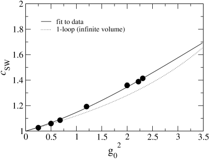
In quenched QCD, the size of the correction is smaller than 5% for all availble data, and we use all data to obtain

$$c_{\rm SW}(g^{2}_{0},L^{*}) = 1+0.113\,g^{2}_{0}+0.0371(54)\,(g^{2}_{0})^{2}-0.0036(26)\,(g^{2}_{0})^{3},\ \ \ \ (\chi^{2}/{\rm dof}=4.09),$$ (66)

$$\kappa_{c}(g^{2}_{0},L^{*}) = 1/8+0.003681192\,g^{2}_{0}+0.000293(37)\,(g^{2}_{0})^{2}$$ (67)

$$\ \ \ \ \ \ -0.000053(65)\,(g^{2}_{0})^{3}+0.000008(24)\,(g^{2}_{0})^{4},\ \ \ (\chi^{2}/{\rm dof}=0.46).$$

In Ref. Aoki:2003sj , the authors performed a one-loop determination of $c_{\rm SW}^{(1)}$ with conventional perturbation theory, and reported a very precise value $c_{\rm SW}^{(1)}$=0.11300591(1) in the infinite volume limit. Changes in our results due to the use of this value in above analyses are expected to be negligibly small.

V Systematic errors

There are two sources of systematic errors in our analysis, both related to the conversion to a fixed physical length scale $L^{*}$, one being the use of the two-loop $\beta$ function to estimate $L^{*}$ as a function of $g^{2}_{0}$, and the second being the use of one-loop perturbation theory for correcting the value of $c_{\rm SW}$ from $L$ to $L^{*}$.

In order to examine the magnitude of uncertainties from the first error, we go through the analysis using the three-loop $\beta$ function. Since the three-loop term of the lattice $\beta$ function is not available for the RG-improved gauge action, we take the value for the plaquette gauge action. Thus the following argument is only semi-quantitatively valid. In this case, Eq. (47) is replaced with

$$a\Lambda_{L} = \exp\left(-\frac{1}{2b_{0}g_{0}^{2}}\right)(b_{0}g^{2}_{0})^{-b_{1}/2b_{0}^{2}}\times\left(1+qg^{2}_{0}\right),$$ (68)

where $q$=0.18960350(1), 0.4529(1), and 0.6138(2) for $N_{f}$=0, 2, and 3 Bode:2001uz , respectively. With this function, we estimate $L^{*}/a$, $\delta c_{\rm SW}$, and $\delta\kappa_{c}$ with $N_{f}$=3, which are tabulated in Table 14. Comparing with Table 2, it is found that $L^{*}/a$ changes significantly while the changes in $\delta c_{\rm SW}$ and $\delta\kappa_{c}$ are at most a few percent and hence small. Thus we conclude that the uncertainty from scaling violation in the lattice spacing is negligible.

In order to discuss the uncertainty of one-loop corrections, we write $c_{\rm SW}(g^{2}_{0},L^{*})$ determined through our procedure as

$$c_{\rm SW}(g^{2}_{0},L^{*}) = c_{\rm SW}(g^{2}_{0},\infty)+c^{(0)}\,(a/L^{*})+g_{0}^{2}\,c^{(1)}(a/L^{*})+g_{0}^{4}\,c^{(2)}(a/L^{*})$$ (69)

$$+g_{0}^{4}\left(\,c^{(2)}(a/L)-c^{(2)}(a/L^{*})\right)+O(g_{0}^{6}).$$

In other words, Eq. (69) represents the difference between $c_{\rm SW}(g^{2}_{0},L^{*})$ and $c_{\rm SW}(g^{2}_{0},\infty)$ in terms of perturbative series with coefficients $c^{(i)}(a/L)$, where $c^{(i)}(a/L)$ vanishes as $L\rightarrow\infty$. Since we have corrected the mismatch between $c_{\rm SW}(g^{2}_{0},L/a)$ and $c_{\rm SW}(g^{2}_{0},L^{*}/a)$ only at the tree- and one-loop level, the unwanted $a/L$ dependence remains at two-loop and higher. Replacing $c_{\rm SW}^{\rm sim}$ in Eq. (42) with Eq. (69), we obtain

$$Q-Q^{\rm latt}(a) = \bigg{(}c^{(0)}(a/L^{*})+g^{2}_{0}\,c^{(1)}(a/L^{*})+g_{0}^{4}\,c^{(2)}(a/L^{*})\bigg{)}\cdot(a\Lambda_{\rm QCD})$$ (70)

$$+g_{0}^{4}\,\big{(}c^{(2)}(a/L)-c^{(2)}(a/L^{*})\big{)}\cdot(a\Lambda_{\rm QCD})+O(g_{0}^{6}\,a\Lambda_{\rm QCD}\,a/L)+O(a^{2}\Lambda_{\rm QCD}^{2}),$$

where we omit an unknown $O(1)$ overall coefficient $q$, because it is not relevant in the following discussion. If you expand $c^{(i)}(a/L^{(*)})$ around $a/L^{(*)}=0$, the first term in Eq. (70) behaves $\sim a^{2}\Lambda_{\rm QCD}/L^{*}\sim O(a^{2})$ because $L^{*}$ is fixed. The second term behaves like $\sim g_{0}^{4}(a/L-a/L^{*})(a\Lambda_{\rm QCD})$, which gives $O(a)$ scaling violation because $a/L$ is fixed. As a results, the leading scaling violation could be $O(a)$ rather than $O(a^{2})$. However it should be emphasized that when we obtain the interpolation formula we only used the weak coupling and strong coupling regions because in these regions the perturbative errors are expected to be under control for the following reasons. In the weak coupling region, $L/a$ and $L^{*}/a$ are different by several orders of magnitude, but the coupling is very small, and hence the size of $O(g^{4}(a/L-a/L^{*})(a\Lambda_{\rm QCD}))$ is expected to be as small as the size of the one-loop corrections. On the other hand, in the strong coupling region, $L/a$ and $L^{*}/a$ are close to each other, and again the remaining $O(a)$ scaling violation, $O(g^{4}(a/L-a/L^{*})(a\Lambda_{\rm QCD}))$, should be small. We also saw in Sec. IV.2 that the size of perturbative errors is roughly the same as that of the one-loop correction itself.

Most importantly, at our strongest and the second strongest couplings around which large-scale simulations are performed, there are no perturbative errors in $c_{\rm SW}$ due to our choice of $L^{*}$ and interpolation to $L^{*}$ at the second strongest couplings. Thus we believe $O(a)$ scaling violations are well below $O(a^{2})$, though we need to check this in future work.

VI Conclusion

In this work, we have performed a nonperturbative determination of the $O(a)$-improvement coefficient $c_{\rm SW}$ of the Wilson quark action with the RG-improved gauge action for $N_{f}$=3, 2, and 0 flavor QCD. The corrections at finite lattice size turn out to be sizable, and are taken into account by modifying the improvement condition and carrying out the determination at a fixed physical length scale of $L^{*}$. While we have to resort to perturbation theory to incorporate the corrections, we have attempted to choose $L^{*}$ at a moderately strong coupling, close to the range of lattice sizes of order $a^{-1}\sim 2$ GeV where physics simulations are practically made, so that their magnitude are reasonably under control.

Using the data for $c_{\rm SW}$ thus obtained over a wide range of $\beta$, we have determined the interpolation formulas, given in Eqs. (60), (63) and (66), which represent the main results of this work. These results do depend on $L^{*}$ chosen, but the removal of $O(a)$ scaling violations in physical observables hold independent of the value of $L^{*}$.

As a byproduct, we have also obtained the interpolation formula for $\kappa_{c}$, Eqs. (61), (65) and (67), which may be useful to locate simulation points.

The three-flavor results reported here are already being used in a large-scale simulation aiming to carry out a systematic evaluation of hadronic observables for the realistic quark spectrum incorporating the dynamical up, down and strange quarks. The preliminary results have been reported in Refs. Kaneko:2003re .

Table 1: Finite-size coefficients in Eqs. (54)–(57).

$c_{\rm SW}^{(0)}$		$c_{\rm SW}^{(1)}$
			$N_{f}=0$	$N_{f}=2$	$N_{f}=3$
$a_{1}$	$-$3.4415	$c_{1}$	$-$4.5736	$-$6.2641	$-$7.1094
$a_{2}$	$-$5.0248	$c_{2}$	$-$3.3402	$-$8.0488	$-$10.403
$a_{3}$	11.1475	$d_{1}$	$-$1.1681	$-$1.5466	$-$1.7359
$b_{1}$	$-$3.9702	$d_{2}$	$-$8.9448	$-$14.306	$-$16.987
$\kappa_{c}^{(0)}$		$\kappa_{c}^{(1)}$
			$N_{f}=0$	$N_{f}=2$	$N_{f}=3$
$k_{1}$	0.260982$\times 10^{-6}$	$l_{1}$	0.101302$\times 10^{-2}$	$-$0.224650$\times 10^{-2}$	$-$0.387626$\times 10^{-2}$
$k_{2}$	$-$0.845333$\times 10^{-5}$	$l_{2}$	0.162496$\times 10^{-1}$	0.862878$\times 10^{-2}$	0.481835$\times 10^{-2}$
$k_{3}$	$-$0.103610$\times 10^{-1}$	$m_{1}$	0.547826$\times 10^{-3}$	$-$0.507665$\times 10^{-3}$	$-$0.155835$\times 10^{-3}$
$k_{4}$	0.751742$\times 10^{-2}$	$m_{2}$	0.882220$\times 10^{-2}$	$-$0.136413$\times 10^{-2}$	$-$0.645729$\times 10^{-2}$

Table 2: Inverse coupling $\beta$ and lattice size $L/a$ chosen for the three-flavor QCD simulation. $L^{*}/a$ is estimated by the two-loop $\beta$ function assuming $L^{*}/a=6$ at $\beta$=1.9. Finite-size corrections $\delta c_{\rm SW}$ and $\delta\kappa_{c}$ calculated with Eqs.(52) and(53) are also shown.

$\beta$	$L/a$	$L^{*}/a$	$\delta c_{\rm SW}(g^{2}_{0},L/a;L^{*}/a)$	$\delta\kappa_{c}(g^{2}_{0},L/a;L^{*}/a)$
12.00	8	7.51$\times 10^{6}$	5.51$\times 10^{-3}$	6.35$\times 10^{-5}$
8.85	8	8.46$\times 10^{4}$	1.42$\times 10^{-2}$	7.95$\times 10^{-5}$
5.00	8	3.81$\times 10^{2}$	5.14$\times 10^{-2}$	1.23$\times 10^{-4}$
3.00	8	2.50$\times 10^{1}$	1.14$\times 10^{-1}$	6.80$\times 10^{-5}$
2.60	8	1.48$\times 10^{1}$	1.08$\times 10^{-1}$	1.34$\times 10^{-5}$
2.40	8	1.14$\times 10^{1}$	8.70$\times 10^{-2}$	$-$8.82$\times 10^{-6}$
2.20	8	8.78	3.42$\times 10^{-2}$	$-$9.84$\times 10^{-6}$
2.10	8	7.73	$-$1.59$\times 10^{-2}$	5.70$\times 10^{-6}$
2.00	8	6.81	$-$9.36$\times 10^{-2}$	3.85$\times 10^{-5}$
2.00	6	6.81	1.10$\times 10^{-1}$	$-$5.08$\times 10^{-5}$
1.90	6	6	0	0

Table 3: Same as Table 2, but for two-flavor QCD.

$\beta$	$L/a$	$L^{*}/a$	$\delta c_{\rm SW}(L/a;L^{*}/a)$	$\delta\kappa(L/a;L^{*}/a)$
12.00	8	2.35$\times 10^{6}$	2.43$\times 10^{-3}$	5.93$\times 10^{-5}$
8.85	8	3.66$\times 10^{4}$	1.01$\times 10^{-2}$	7.38$\times 10^{-5}$
5.00	8	2.45$\times 10^{2}$	4.63$\times 10^{-2}$	1.08$\times 10^{-4}$
3.00	8	1.98$\times 10^{1}$	9.51$\times 10^{-2}$	2.69$\times 10^{-5}$
2.60	8	1.22$\times 10^{1}$	7.84$\times 10^{-2}$	$-$1.81$\times 10^{-5}$
2.20	8	7.58	$-$2.11$\times 10^{-2}$	1.41$\times 10^{-5}$
2.10	8	6.74	$-$8.24$\times 10^{-2}$	6.14$\times 10^{-5}$
2.10	6	6.74	8.37$\times 10^{-2}$	$-$7.04$\times 10^{-5}$
2.00	6	6	0	0

Table 4: Same as Table 2, but for quenched QCD.

$\beta$	$L/a$	$L^{*}/a$	$\delta c_{\rm SW}(L/a;L^{*}/a)$	$\delta\kappa(L/a;L^{*}/a)$
24.00	8	3.09$\times 10^{11}$	$-$1.11$\times 10^{-2}$	3.47$\times 10^{-5}$
12.00	8	2.41$\times 10^{5}$	$-$3.70$\times 10^{-3}$	5.08$\times 10^{-5}$
8.85	8	6.33$\times 10^{3}$	2.24$\times 10^{-3}$	6.18$\times 10^{-5}$
5.00	8	8.04$\times 10^{1}$	3.80$\times 10^{-2}$	6.29$\times 10^{-5}$
3.00	8	9.12	2.07$\times 10^{-2}$	$-$2.68$\times 10^{-5}$
2.70	8	6.66	$-$4.81$\times 10^{-2}$	8.79$\times 10^{-5}$
2.70	6	6.66	3.98$\times 10^{-2}$	$-$8.40$\times 10^{-5}$
2.60	6	6	0	0

Table 5: Results for $aM$ and $a\Delta M$ for three-flavor QCD. The acceptance rates for the MD and the noisy Metropolis test are shown together with the number of MD steps per trajectory and the order of the polynomial $N_{\rm poly}$ used in the noisy Metropolis test. The final column gives the number of trajetories accumulated.

$c_{\rm SW}$	$\kappa$	$aM$	$a\Delta M$	$P_{\rm acc}[N_{\rm MD}]$	$P_{\rm corr}[N_{\rm poly}]$	$N_{\rm traj}$
$\beta=12.00$, $L/a=8$
1.00	0.12659	0.01235(13)	0.00101(13)	0.73(2)[100]	0.983(5)[100]	1600
	0.12676	0.006906(91)	0.00072(13)	0.75(1)[100]	0.979(4)[100]	1600
	0.12693	0.00149(13)	0.00087(14)	0.73(2)[100]	0.973(5)[100]	1600
	0.12709	$-$0.00368(13)	0.00092(16)	0.75(1)[100]	0.970(5)[100]	1600
1.05	0.12659	0.008565(98)	$-$0.00009(18)	0.72(2)[100]	0.984(4)[100]	1600
	0.12676	0.00283(11)	$-$0.00003(13)	0.74(1)[100]	0.968(6)[100]	1600
	0.12693	$-$0.00221(11)	0.00004(17)	0.72(3)[100]	0.969(6)[100]	1600
	0.12709	$-$0.007708(89)	0.00023(10)	0.74(2)[100]	0.955(5)[100]	1600
1.10	0.12659	0.00460(12)	$-$0.00076(13)	0.72(2)[100]	0.981(4)[100]	1600
	0.12676	$-$0.00097(15)	$-$0.00069(22)	0.71(3)[100]	0.972(4)[100]	1600
	0.12693	$-$0.00625(21)	$-$0.00073(16)	0.74(2)[100]	0.953(9)[100]	1600
	0.12709	$-$0.01161(17)	$-$0.00070(13)	0.73(2)[100]	0.94(2)[100]	1600
$\beta=8.85$, $L/a=8$
1.0141	0.12698	0.02316(13)	0.00094(15)	0.68(2)[80]	0.989(3)[100]	2000
	0.12730	0.01311(11)	0.00104(18)	0.66(2)[80]	0.988(4)[100]	2000
	0.12762	0.00309(12)	0.00102(15)	0.71(2)[80]	0.969(5)[100]	2000
	0.12826	$-$0.01734(10)	0.00092(16)	0.70(1)[80]	0.943(6)[110]	2000
1.0350	0.12698	0.02121(11)	0.00060(12)	0.70(2)[80]	0.990(2)[100]	2000
	0.12730	0.01119(16)	0.00057(17)	0.71(1)[80]	0.985(3)[100]	2000
	0.12762	0.00080(13)	0.00060(16)	0.70(2)[80]	0.972(4)[100]	2000
	0.12826	$-$0.01948(13)	0.00055(15)	0.71(2)[80]	0.937(6)[110]	2000
1.0559	0.12698	0.01903(14)	0.00013(14)	0.69(2)[80]	0.987(4)[100]	2000
	0.12730	0.00896(11)	0.00033(10)	0.68(1)[80]	0.975(4)[100]	2000
	0.12762	$-$0.00130(11)	0.00024(20)	0.69(2)[80]	0.964(5)[100]	2000
	0.12826	$-$0.02166(13)	0.00039(10)	0.70(2)[80]	0.928(7)[110]	2000
1.0800	0.12719	0.00983(15)	$-$0.00013(15)	0.69(2)[80]	0.990(2)[120]	2000
	0.12753	$-$0.00078(11)	0.00007(12)	0.68(2)[80]	0.989(3)[130]	2000
1.1000	0.12713	0.00982(35)	$-$0.00041(19)	0.68(2)[80]	0.990(3)[110]	2000
	0.12747	$-$0.00121(11)	$-$0.00039(14)	0.69(1)[80]	0.986(3)[120]	2000
$\beta=5.00$, $L/a=8$
1.08	0.12958	0.01031(33)	0.00073(22)	0.72(1)[64]	0.982(3)[100]	2200
	0.12974	0.00553(17)	0.00082(29)	0.77(2)[64]	0.968(4)[100]	2200
	0.12989	0.00049(35)	0.00060(25)	0.74(2)[64]	0.970(4)[100]	2200
	0.13004	$-$0.00377(20)	0.00070(19)	0.74(2)[64]	0.962(5)[100]	2200
1.13	0.12932	0.01027(26)	0.00039(22)	0.73(1)[64]	0.976(6)[100]	2200
	0.12948	0.00541(24)	0.00043(27)	0.73(1)[64]	0.975(4)[100]	2200
	0.12963	0.00030(24)	0.00024(21)	0.77(1)[64]	0.964(7)[100]	2200
	0.12978	$-$0.00428(29)	0.00042(37)	0.74(1)[64]	0.950(6)[100]	2200
1.18	0.12907	0.01002(22)	$-$0.00071(20)	0.76(2)[64]	0.982(3)[100]	2200
	0.12922	0.00489(25)	$-$0.00105(22)	0.73(2)[64]	0.974(4)[100]	2200
	0.12937	0.00043(43)	$-$0.00074(21)	0.75(1)[64]	0.970(4)[100]	2200
	0.12952	$-$0.00441(28)	$-$0.00089(21)	0.76(1)[64]	0.958(6)[100]	2200
$\beta=3.00$, $L/a=8$
1.20	0.13281	0.02798(33)	0.00099(26)	0.770(9)[50]	0.988(2)[100]	4300
	0.13311	0.01769(47)	0.00036(57)	0.77(1)[50]	0.978(3)[100]	4000
	0.13341	0.00813(46)	0.00044(33)	0.78(1)[50]	0.960(4)[100]	4000
	0.13370	$-$0.00036(41)	0.00104(40)	0.77(1)[50]	0.937(5)[100]	3800
1.25	0.13235	0.02774(42)	$-$0.00015(61)	0.78(1)[50]	0.986(4)[100]	4200
	0.13265	0.01820(52)	0.00003(40)	0.76(1)[50]	0.980(3)[100]	3800
	0.13294	0.00940(38)	0.00004(36)	0.77(1)[50]	0.960(3)[100]	4200
	0.13324	$-$0.00027(40)	$-$0.00029(34)	0.773(9)[50]	0.948(5)[100]	3900
1.30	0.13190	0.02742(65)	$-$0.00052(28)	0.76(1)[50]	0.990(2)[100]	4200
	0.13219	0.01713(64)	$-$0.00040(36)	0.77(2)[50]	0.980(2)[100]	4200
	0.13248	0.00915(54)	$-$0.00066(67)	0.78(2)[50]	0.962(3)[100]	3900
	0.13278	$-$0.00008(41)	0.00031(64)	0.77(1)[50]	0.945(6)[100]	4000
1.35	0.13145	0.02697(35)	$-$0.00098(46)	0.77(1)[50]	0.988(3)[100]	4300
	0.13174	0.01643(70)	$-$0.00075(44)	0.770(8)[50]	0.979(4)[100]	4100
	0.13203	0.00800(43)	$-$0.00092(58)	0.76(1)[50]	0.972(3)[100]	4100
	0.13232	$-$0.00079(38)	$-$0.00109(38)	0.77(1)[50]	0.947(4)[100]	4000
$\beta=2.60$, $L/a=8$
1.20	0.13531	0.02110(64)	0.00168(38)	0.878(9)[64]	0.979(3)[110]	4500
	0.13550	0.01528(44)	0.00142(85)	0.879(6)[64]	0.972(3)[110]	4500
	0.13574	0.00810(69)	0.00170(43)	0.87(1)[64]	0.966(6)[120]	4500
	0.13594	0.00140(72)	0.00158(62)	0.882(7)[64]	0.965(8)[130]	4500
1.27	0.13454	0.02061(53)	0.00073(91)	0.870(6)[64]	0.983(2)[110]	4500
	0.13473	0.01512(73)	0.00218(47)	0.881(6)[64]	0.978(2)[110]	4500
	0.13496	0.00721(52)	0.00102(48)	0.883(10)[64]	0.971(5)[120]	4500
	0.13516	0.00327(73)	0.00039(53)	0.883(6)[64]	0.972(3)[130]	4500
1.34	0.13378	0.02177(75)	$-$0.00006(57)	0.883(6)[64]	0.984(2)[110]	4500
	0.13420	0.00830(57)	$-$0.00004(45)	0.872(6)[64]	0.972(3)[120]	4500
	0.13440	0.0018(11)	0.00031(44)	0.876(9)[64]	0.975(2)[130]	4500
	0.13473	$-$0.00968(93)	$-$0.00007(34)	0.880(6)[64]	0.903(5)[110]	4500
1.41	0.13303	0.02040(50)	$-$0.00055(43)	0.874(7)[64]	0.983(2)[110]	4500
	0.13322	0.01375(64)	$-$0.00042(67)	0.874(7)[64]	0.979(3)[110]	4500
	0.13344	0.00792(81)	$-$0.00064(37)	0.873(9)[64]	0.975(3)[120]	4500
	0.13364	0.00116(66)	$-$0.00022(50)	0.882(6)[64]	0.964(3)[130]	4500
1.48	0.13277	0.0036(10)	$-$0.00109(49)	0.883(6)[64]	0.978(3)[130]	5000
	0.13301	$-$0.00316(79)	$-$0.00085(34)	0.872(6)[64]	0.979(2)[150]	5000
1.55	0.13202	0.00476(58)	$-$0.00218(36)	0.873(7)[64]	0.980(2)[130]	5000
	0.13226	$-$0.00270(73)	$-$0.00195(48)	0.879(10)[64]	0.973(3)[140]	5000
$\beta=2.40$, $L/a=8$
1.3	0.135917	0.0211(39)	0.00162(74)	0.819(7)[50]	0.974(2)[110]	10000
	0.136152	0.01146(50)	0.00011(100)	0.819(5)[50]	0.971(2)[120]	10000
	0.136387	0.00276(49)	0.00100(29)	0.82(1)[50]	0.947(2)[120]	10000
1.4	0.134882	0.01207(50)	0.00022(60)	0.815(5)[50]	0.974(2)[120]	10000
	0.135113	0.00466(45)	0.00034(50)	0.828(5)[50]	0.954(2)[120]	10000
1.5	0.133410	0.0206(10)	$-$0.00040(30)	0.823(4)[50]	0.983(2)[110]	10000
	0.133636	0.01300(56)	0.00027(68)	0.828(5)[50]	0.979(2)[120]	10000
	0.133862	0.00584(49)	$-$0.00095(39)	0.827(5)[50]	0.966(2)[120]	10000
1.6	0.132400	0.0151(12)	$-$0.00210(81)	0.82(1)[50]	0.980(2)[120]	11900
	0.132680	0.00567(70)	$-$0.00194(55)	0.825(5)[50]	0.966(2)[120]	11900
1.7	0.131230	0.01385(71)	$-$0.00236(54)	0.888(5)[64]	0.983(1)[120]	10700
	0.131510	0.0047(13)	$-$0.00321(28)	0.886(7)[64]	0.978(1)[130]	10700
$\beta=2.20$, $L/a=8$
1.3	0.138247	0.01685(90)	0.00161(63)	0.840(5)[50]	0.958(2)[120]	16500
	0.138487	0.0100(15)	0.00144(36)	0.836(3)[50]	0.946(3)[130]	16500
	0.138729	0.00128(62)	0.00149(45)	0.843(4)[50]	0.919(3)[140]	16500
1.5	0.135400	0.01877(64)	$-$0.00028(38)	0.844(4)[50]	0.973(1)[120]	16000
	0.135654	0.01083(46)	$-$0.00004(36)	0.844(4)[50]	0.965(2)[130]	16500
	0.135885	0.00285(55)	0.00079(51)	0.841(4)[50]	0.951(2)[140]	16500
1.7	0.132712	0.01913(70)	$-$0.00148(29)	0.846(5)[50]	0.983(1)[120]	16500
	0.132934	0.01226(45)	$-$0.00198(45)	0.844(8)[50]	0.977(2)[130]	16500
	0.133156	0.00494(49)	$-$0.00205(50)	0.834(5)[50]	0.968(2)[140]	16500
1.9	0.130170	0.02045(54)	$-$0.00385(32)	0.843(6)[50]	0.984(1)[120]	16100
	0.130370	0.01248(76)	$-$0.00342(30)	0.840(4)[50]	0.984(2)[130]	16100
	0.130570	0.00561(55)	$-$0.00322(32)	0.841(4)[50]	0.977(1)[140]	16100
$\beta=2.10$, $L/a=8$
1.5	0.1355	0.0579(12)	0.00066(57)	0.850(4)[50]	0.979(3)[80]	14500
	0.1358	0.0500(15)	0.00011(44)	0.847(4)[50]	0.9877(10)[100]	14500
	0.1360	0.04380(77)	0.00033(44)	0.855(4)[50]	0.984(1)[100]	14400
	0.1362	0.0386(10)	0.00047(56)	0.851(6)[50]	0.978(2)[100]	14500
1.6	0.1340	0.06167(75)	$-$0.00027(49)	0.854(5)[50]	0.986(2)[80]	14500
	0.1344	0.04811(59)	0.00039(83)	0.848(5)[50]	0.9888(10)[100]	14500
	0.1346	0.04179(72)	$-$0.00035(76)	0.850(4)[50]	0.985(1)[100]	14500
1.7	0.1326	0.05964(58)	$-$0.00132(47)	0.853(5)[50]	0.987(1)[80]	14500
	0.1329	0.04952(50)	$-$0.00128(33)	0.850(4)[50]	0.987(2)[90]	14500
	0.1331	0.04393(48)	$-$0.00145(32)	0.854(3)[50]	0.988(1)[100]	14500
	0.1333	0.03752(54)	$-$0.00018(31)	0.849(3)[50]	0.982(2)[100]	14500
	0.1335	0.02976(87)	$-$0.00096(31)	0.856(3)[50]	0.974(1)[100]	14500
1.8	0.1315	0.05054(44)	$-$0.00192(33)	0.850(4)[50]	0.9889(9)[90]	14500
	0.1318	0.04101(59)	$-$0.00182(35)	0.844(3)[50]	0.9883(10)[100]	14500
	0.1321	0.03149(47)	$-$0.00176(41)	0.847(4)[50]	0.983(2)[110]	14500
	0.1324	0.01956(59)	$-$0.00148(33)	0.850(4)[50]	0.980(1)[120]	14500
$\beta=2.00$, $L/a=8$
1.5	0.1383550	0.0276(15)	0.00020(44)	0.863(3)[50]	0.961(2)[130]	24500
	0.1386672	0.0176(12)	0.00082(56)	0.857(3)[50]	0.928(2)[140]	21500
	0.1388000	0.0138(13)	0.00034(58)	0.853(3)[50]	0.914(7)[160]	21200
1.6	0.1364310	0.0360(10)	0.00036(60)	0.858(4)[50]	0.9912(9)[140]	20000
	0.1367500	0.02618(98)	$-$0.0011(10)	0.857(4)[50]	0.982(1)[150]	20000
	0.1370700	0.0156(12)	0.00049(52)	0.857(7)[50]	0.961(2)[160]	20000
1.7	0.1348740	0.03723(61)	$-$0.00134(41)	0.856(3)[50]	0.9932(9)[140]	20000
	0.1354309	0.01588(70)	$-$0.00073(30)	0.861(3)[50]	0.950(2)[130]	24500
	0.1354980	0.01435(93)	$-$0.00037(46)	0.859(3)[50]	0.971(1)[160]	20000
	0.1356000	0.01043(82)	$-$0.00072(58)	0.861(4)[50]	0.951(2)[150]	20300
1.8	0.1333520	0.03533(61)	$-$0.00095(40)	0.859(3)[50]	0.9936(6)[140]	20000
	0.1336570	0.02441(57)	$-$0.00129(33)	0.863(3)[50]	0.9899(8)[150]	20000
	0.1339620	0.01374(65)	$-$0.00050(51)	0.853(5)[50]	0.978(1)[160]	20000
1.9	0.1320578	0.02843(57)	$-$0.00237(38)	0.860(3)[50]	0.977(1)[110]	24500
	0.1323422	0.01918(68)	$-$0.00166(42)	0.860(2)[50]	0.976(1)[130]	24500
	0.1326278	0.01016(60)	$-$0.00183(39)	0.858(3)[50]	0.945(2)[130]	24500
2.0	0.1308300	0.0208(13)	$-$0.00357(75)	0.853(6)[50]	0.989(2)[150]	5400
	0.1311100	0.01208(82)	$-$0.00310(40)	0.860(7)[50]	0.983(2)[160]	7300
2.1	0.1293800	0.02589(84)	$-$0.00391(65)	0.859(8)[50]	0.996(2)[150]	5400
	0.1296600	0.01483(96)	$-$0.00406(79)	0.855(5)[50]	0.988(2)[160]	7300
$\beta=2.00$, $L/a=6$
1.30	0.1400	0.1002(43)	0.0055(15)	0.925(3)[50]	0.9998(2)[120]	11200
	0.1400	0.1017(33)	0.00346(89)	0.926(3)[50]	1.0000(0)[120]	11200
	0.1405	0.0871(30)	0.00390(95)	0.923(2)[50]	0.9993(2)[120]	14500
	0.1405	0.0890(29)	0.0030(11)	0.926(2)[50]	0.9991(5)[120]	14500
	0.1410	0.0669(28)	0.0033(11)	0.922(3)[50]	0.9974(6)[120]	15000
	0.1410	0.0721(30)	0.0045(15)	0.922(2)[50]	0.9974(8)[120]	15000
	0.1415	0.0505(26)	0.0037(11)	0.922(4)[50]	0.990(1)[120]	15100
	0.1415	0.0508(24)	0.0048(12)	0.923(2)[50]	0.990(1)[120]	15100
1.45	0.1380	0.0752(22)	0.00153(95)	0.925(3)[50]	0.9995(2)[120]	14900
	0.1380	0.0784(17)	0.00126(66)	0.925(3)[50]	0.9994(3)[120]	14900
	0.1385	0.0564(17)	0.00224(73)	0.921(3)[50]	0.9985(4)[120]	14900
	0.1385	0.0568(24)	0.00094(76)	0.922(4)[50]	0.9979(5)[120]	14900
	0.1390	0.0401(20)	$-$0.0001(12)	0.921(2)[50]	0.994(1)[120]	15000
	0.1390	0.0417(21)	0.00173(83)	0.921(3)[50]	0.993(1)[120]	15000
	0.1395	0.0231(17)	0.00128(80)	0.923(5)[50]	0.982(2)[120]	15100
	0.1395	0.0245(23)	0.00238(83)	0.926(3)[50]	0.981(1)[120]	15100
1.60	0.1355	0.0673(20)	0.0021(16)	0.925(4)[50]	0.9994(2)[120]	11200
	0.1355	0.0698(16)	$-$0.00090(78)	0.924(3)[50]	0.9998(2)[120]	11200
	0.1360	0.0530(17)	$-$0.00053(56)	0.920(3)[50]	0.9983(6)[120]	15000
	0.1360	0.0535(14)	$-$0.0004(14)	0.925(3)[50]	0.9990(3)[120]	15000
	0.1365	0.0340(19)	0.0008(10)	0.926(2)[50]	0.9957(8)[120]	15000
	0.1365	0.0347(15)	0.00078(62)	0.925(3)[50]	0.9971(5)[120]	15000
	0.1370	0.0165(14)	$-$0.00013(69)	0.922(3)[50]	0.988(1)[120]	15000
	0.1370	0.0171(16)	$-$0.0004(12)	0.923(2)[50]	0.9888(10)[120]	15000
1.75	0.1330	0.0682(37)	$-$0.00223(95)	0.920(7)[50]	1.0000(0)[120]	3400
	0.1330	0.0683(20)	$-$0.0016(10)	0.927(7)[50]	0.9997(3)[120]	3400
	0.1335	0.05035(96)	$-$0.00293(66)	0.925(3)[50]	0.9996(3)[120]	14500
	0.1335	0.05242(96)	$-$0.00187(64)	0.923(3)[50]	0.9995(2)[120]	14500
	0.1340	0.0339(10)	$-$0.00088(59)	0.927(3)[50]	0.9985(5)[120]	15000
	0.1340	0.0350(11)	$-$0.0025(13)	0.924(3)[50]	0.9983(5)[120]	15000
	0.1345	0.0164(15)	$-$0.0026(10)	0.920(3)[50]	0.9948(6)[120]	15000
	0.1345	0.0197(15)	$-$0.00095(70)	0.920(3)[50]	0.994(1)[120]	15000
$\beta=1.90$, $L/a=6$
1.4	0.1410	0.1315(62)	0.00112(92)	0.930(2)[50]	0.9997(1)[120]	24000
	0.1410	0.1338(41)	0.0008(13)	0.923(2)[50]	0.9997(1)[120]	23900
	0.1415	0.1103(64)	0.0006(12)	0.928(2)[50]	0.9985(4)[120]	24000
	0.1415	0.1136(36)	0.00144(94)	0.927(2)[50]	0.9989(2)[120]	24000
	0.1420	0.0857(25)	0.0028(10)	0.930(3)[50]	0.9930(8)[120]	24100
	0.1420	0.0876(31)	0.00166(90)	0.923(2)[50]	0.9945(5)[120]	24100
1.8	0.1340	0.0878(25)	$-$0.00021(84)	0.929(3)[50]	1.0000(0)[120]	15100
	0.1340	0.0900(21)	$-$0.00174(58)	0.928(3)[50]	1.0000(0)[120]	15100
	0.1345	0.0710(21)	$-$0.00159(69)	0.926(3)[50]	0.9994(2)[120]	24000
	0.1345	0.0733(14)	$-$0.00193(55)	0.929(2)[50]	0.9995(3)[120]	24000
	0.1350	0.0520(24)	$-$0.00136(59)	0.929(2)[50]	0.9973(3)[120]	24100
	0.1350	0.0535(21)	$-$0.00045(76)	0.928(2)[50]	0.9976(6)[120]	24100
	0.1355	0.0307(16)	$-$0.00102(68)	0.926(2)[50]	0.9888(7)[120]	24100
	0.1355	0.0309(14)	$-$0.00108(55)	0.926(2)[50]	0.9895(8)[120]	24100
2.2	0.1280	0.06146(84)	$-$0.00601(53)	0.928(2)[50]	0.99991(9)[120]	22700
	0.1280	0.06303(92)	$-$0.00699(67)	0.926(2)[50]	0.9998(1)[120]	22700
	0.1285	0.04376(79)	$-$0.00734(52)	0.928(2)[50]	0.9993(2)[120]	23600
	0.1285	0.04434(83)	$-$0.00594(51)	0.928(2)[50]	0.9996(1)[120]	23600
	0.1290	0.02540(87)	$-$0.00681(84)	0.929(2)[50]	0.9976(6)[120]	24100
	0.1290	0.02607(99)	$-$0.00585(67)	0.924(2)[50]	0.9976(4)[120]	24100
	0.1295	0.00747(99)	$-$0.0044(16)	0.925(2)[50]	0.9916(8)[120]	24100
	0.1295	0.0084(15)	$-$0.00649(46)	0.928(2)[50]	0.9922(6)[120]	24100
2.5	0.1240	0.0535(12)	$-$0.01090(60)	0.926(2)[50]	0.99990(7)[120]	22200
	0.1240	0.0539(12)	$-$0.01076(50)	0.927(2)[50]	0.9997(2)[120]	22200
	0.1245	0.0372(13)	$-$0.01083(49)	0.929(2)[50]	0.9996(1)[120]	24000
	0.1250	0.01913(94)	$-$0.01152(87)	0.926(2)[50]	0.9985(3)[120]	24000
	0.1250	0.0198(11)	$-$0.01144(38)	0.925(2)[50]	0.9986(3)[120]	24100
	0.1255	0.00201(98)	$-$0.01160(49)	0.924(2)[50]	0.9937(7)[120]	24100
	0.1255	$-$0.00014(87)	$-$0.01100(44)	0.923(2)[50]	0.9932(8)[120]	24100

Table 6: Same as Table LABEL:tab:Nf3MandDM for two-flavor QCD.

$c_{\rm SW}$	$\kappa$	$aM$	$a\Delta M$	$P_{\rm acc}[N_{\rm MD}]$	$N_{\rm traj}$
$\beta=12.00$, $L/a=8$
1.00	0.12659	0.01266(15)	0.00082(16)	0.75(3)[100]	1500
	0.12676	0.007137(77)	0.00083(14)	0.74(2)[100]	1500
	0.12693	0.00180(16)	0.00115(16)	0.73(2)[100]	1500
	0.12709	$-$0.003231(98)	0.00070(13)	0.75(2)[100]	1500
1.05	0.12659	0.00882(14)	0.00003(20)	0.71(3)[100]	1500
	0.12676	0.00317(11)	0.00019(14)	0.73(2)[100]	1500
	0.12693	$-$0.00199(11)	0.00016(14)	0.70(2)[100]	1500
	0.12709	$-$0.00735(16)	$-$0.00008(12)	0.72(2)[100]	1500
1.10	0.12659	0.00498(12)	$-$0.00061(11)	0.74(2)[100]	1500
	0.12676	$-$0.00042(12)	$-$0.00065(15)	0.73(1)[100]	1500
	0.12693	$-$0.00581(11)	$-$0.00069(12)	0.71(2)[100]	1500
	0.12709	$-$0.01119(15)	$-$0.00070(12)	0.74(2)[100]	1500
$\beta=8.85$, $L/a=8$
1.040	0.1270	0.020524(91)	0.00036(11)	0.72(2)[80]	2100
	0.1274	0.00794(13)	0.00056(11)	0.72(2)[80]	2100
	0.1278	$-$0.00470(14)	0.00052(15)	0.70(1)[80]	2100
	0.1282	$-$0.017306(94)	0.00043(14)	0.70(1)[80]	2000
1.055	0.1270	0.019165(83)	0.00044(14)	0.70(2)[80]	2000
	0.1274	0.00665(14)	0.00042(16)	0.70(2)[80]	2000
	0.1278	$-$0.00628(12)	0.00032(18)	0.67(2)[80]	2000
	0.1282	$-$0.01900(12)	0.00025(16)	0.70(2)[80]	2000
1.070	0.1270	0.01758(10)	0.00002(15)	0.70(1)[80]	2000
	0.1274	0.00505(12)	0.00001(18)	0.70(1)[80]	2000
	0.1278	$-$0.00754(14)	0.00027(14)	0.69(2)[80]	2000
	0.1282	$-$0.02057(17)	0.00012(11)	0.70(2)[80]	2000
$\beta=5.00$, $L/a=8$
1.09	0.12954	0.01204(16)	0.00054(26)	0.75(1)[64]	2300
	0.12970	0.00692(23)	0.00068(21)	0.76(2)[64]	2300
	0.12986	0.00198(25)	0.00041(21)	0.74(1)[64]	2300
	0.13002	$-$0.00308(18)	0.00086(43)	0.74(1)[64]	2300
1.13	0.12933	0.01167(21)	$-$0.00005(31)	0.74(2)[64]	2300
	0.12949	0.00691(21)	$-$0.00014(24)	0.75(1)[64]	2300
	0.12965	0.00174(15)	0.00041(19)	0.75(1)[64]	2300
	0.12981	$-$0.00307(24)	$-$0.00013(20)	0.75(1)[64]	2300
1.17	0.12912	0.01164(26)	$-$0.00063(18)	0.76(2)[64]	2300
	0.12928	0.00667(27)	$-$0.00031(28)	0.74(2)[64]	2300
	0.12943	0.00175(32)	$-$0.00076(20)	0.75(1)[64]	2300
	0.12959	$-$0.00338(19)	$-$0.00020(33)	0.75(1)[64]	2300
$\beta=3.00$, $L/a=8$
1.20	0.1332100	0.02195(25)	0.00069(38)	0.780(5)[50]	10500
	0.1333700	0.01674(36)	0.00086(22)	0.767(7)[50]	10500
	0.1335400	0.01165(34)	0.00044(28)	0.77(1)[50]	10500
	0.1337000	0.00685(22)	0.00068(28)	0.762(5)[50]	10500
1.28	0.1324700	0.02175(35)	$-$0.00013(29)	0.774(6)[50]	10500
	0.1326300	0.01668(33)	$-$0.00007(21)	0.773(6)[50]	10500
	0.1327900	0.01168(30)	$-$0.00008(40)	0.781(8)[50]	10500
	0.1329500	0.00649(35)	0.00021(22)	0.766(5)[50]	10500
1.36	0.1317300	0.02146(39)	$-$0.00079(21)	0.769(7)[50]	10500
	0.1318900	0.01644(30)	$-$0.00068(24)	0.771(7)[50]	10500
	0.1320400	0.01156(37)	$-$0.00099(28)	0.777(7)[50]	10500
	0.1322000	0.00675(30)	$-$0.00092(22)	0.779(6)[50]	10500
$\beta=2.60$, $L/a=8$
1.20	0.135574	0.02473(74)	0.00104(62)	0.809(7)[50]	4500
	0.135738	0.0191(12)	0.00161(59)	0.800(8)[50]	4500
	0.135903	0.01522(75)	0.00209(53)	0.808(7)[50]	4500
	0.136068	0.01002(58)	0.00143(93)	0.806(8)[50]	4500
1.25	0.135020	0.02424(81)	0.0015(10)	0.80(1)[50]	4500
	0.135180	0.01912(58)	0.00149(49)	0.811(8)[50]	4500
	0.135340	0.01506(67)	0.00156(56)	0.810(8)[50]	4500
	0.135510	0.00982(59)	0.00150(82)	0.812(7)[50]	4500
1.30	0.134470	0.02492(54)	$-$0.0004(11)	0.800(8)[50]	4500
	0.134630	0.01950(73)	0.00175(52)	0.814(8)[50]	4500
	0.134790	0.01474(63)	$-$0.00007(49)	0.803(7)[50]	4500
	0.134950	0.00949(53)	0.00038(65)	0.804(8)[50]	4500
1.35	0.133920	0.02369(45)	0.00044(47)	0.82(1)[50]	4500
	0.134080	0.0190(10)	$-$0.00040(73)	0.803(7)[50]	4500
	0.134240	0.01426(70)	0.00011(93)	0.82(1)[50]	4500
	0.134400	0.00907(51)	$-$0.00044(57)	0.81(1)[50]	4500
$\beta=2.20$, $L/a=8$
1.35	0.13868	0.01252(59)	0.00182(70)	0.828(3)[50]	37300
	0.13914	$-$0.00310(93)	0.00130(87)	0.834(2)[50]	35900
1.50	0.13654	0.00838(96)	0.00071(72)	0.834(2)[50]	41100
	0.13693	$-$0.00433(75)	0.00003(62)	0.833(2)[50]	39600
1.60	0.13500	0.01012(23)	$-$0.00060(39)	0.839(2)[50]	39900
	0.13543	$-$0.00483(38)	$-$0.00076(68)	0.832(2)[50]	38000
$\beta=2.10$, $L/a=8$
1.38	0.14040	0.00598(95)	0.0007(11)	0.811(2)[50]	145700
	0.14092	$-$0.01094(54)	0.00188(56)	0.810(2)[50]	167500
1.53	0.13741	0.02124(23)	0.00062(65)	0.829(2)[50]	67800
	0.13837	$-$0.00872(53)	0.00074(92)	0.822(2)[50]	58900
1.63	0.13599	0.01371(17)	0.00030(58)	0.830(2)[50]	66400
	0.13648	$-$0.0018(11)	0.00020(57)	0.828(2)[50]	62900
1.73	0.13451	0.01152(32)	$-$0.00008(48)	0.836(1)[50]	104400
	0.13497	$-$0.00317(40)	$-$0.0018(12)	0.833(2)[50]	137100
$\beta=2.10$, $L/a=6$
1.2	0.14347	0.0077(22)	0.0063(21)	0.864(3)[40]	21600
	0.14391	$-$0.0025(21)	0.0079(24)	0.865(4)[40]	26000
1.4	0.13987	0.0125(18)	0.0030(11)	0.868(4)[40]	26000
	0.14021	0.0043(14)	0.0032(17)	0.864(3)[40]	26000
	0.14056	$-$0.0090(23)	0.0025(14)	0.862(4)[40]	26000
1.6	0.13660	0.0073(13)	0.0014(10)	0.869(7)[40]	25200
	0.13683	0.00065(93)	$-$0.00042(78)	0.868(3)[40]	26000
	0.13725	$-$0.0136(16)	$-$0.0002(11)	0.863(2)[40]	25200
1.8	0.13335	0.00825(67)	$-$0.00438(74)	0.867(4)[40]	26000
	0.13362	$-$0.00169(79)	$-$0.00214(84)	0.870(2)[40]	26000
	0.13389	$-$0.0102(10)	$-$0.00278(77)	0.867(4)[40]	28000
2.0	0.13059	$-$0.0001(14)	$-$0.00685(74)	0.870(3)[40]	21600
	0.13090	$-$0.0127(12)	$-$0.0071(10)	0.870(3)[40]	21600
2.4	0.12500	0.0022(17)	$-$0.01283(75)	0.873(3)[40]	21600
	0.12550	$-$0.0148(31)	$-$0.0133(12)	0.865(3)[40]	21600
$\beta=2.00$, $L/a=6$
1.4	0.14279	0.0125(26)	0.0068(17)	0.906(4)[50]	20000
	0.14362	$-$0.0135(21)	0.0033(33)	0.902(3)[50]	25000
1.6	0.13901	0.0131(17)	0.0034(21)	0.914(2)[50]	25000
	0.13936	0.0035(16)	0.00330(91)	0.907(3)[50]	25000
	0.13971	$-$0.0088(16)	0.0009(26)	0.906(4)[50]	25000
1.8	0.13536	0.0113(15)	0.0002(13)	0.918(2)[50]	25000
	0.13588	$-$0.0069(12)	$-$0.0013(22)	0.909(4)[50]	25000
	0.13627	$-$0.0198(45)	0.0006(24)	0.907(7)[50]	25000
2.0	0.13192	0.0116(11)	$-$0.00490(92)	0.918(3)[50]	25000
	0.13221	0.0015(18)	$-$0.0041(14)	0.916(4)[50]	25000
	0.13250	$-$0.0106(12)	$-$0.0033(11)	0.915(2)[50]	25000
2.2	0.12839	0.0207(11)	$-$0.0074(11)	0.921(3)[50]	20000
	0.12902	$-$0.0008(18)	$-$0.0078(12)	0.919(2)[50]	20000
2.6	0.12295	0.01399(86)	$-$0.01330(73)	0.918(3)[50]	21000
	0.12353	$-$0.0093(14)	$-$0.01204(69)	0.921(3)[50]	21000

Table 6: (Continued)

Table 7: Same as Table LABEL:tab:Nf3MandDM for quenched QCD.

$c_{\rm SW}$	$\kappa$	$aM$	$a\Delta M$	$P_{\rm acc}[N_{\rm MD}]$	$N_{\rm traj}$
$\beta=24.00$, $L/a=8$
1.00	0.12567	0.009136(59)	0.000714(97)	0.67(1)[128]	3100
	0.12584	0.003733(51)	0.000545(69)	0.67(1)[128]	3100
	0.12600	$-$0.00139(11)	0.000525(96)	0.65(2)[128]	3100
	0.12617	$-$0.006783(76)	0.000567(79)	0.66(1)[128]	3100
1.03	0.12567	0.007822(63)	0.000078(90)	0.67(1)[128]	3100
	0.12584	0.002319(54)	0.000054(70)	0.67(1)[128]	3100
	0.12600	$-$0.002756(68)	0.000167(81)	0.67(1)[128]	3100
	0.12617	$-$0.008282(63)	$-$0.000028(77)	0.67(1)[128]	3100
1.06	0.12567	0.006427(46)	$-$0.000334(63)	0.67(1)[128]	3100
	0.12584	0.000984(78)	$-$0.000317(76)	0.68(1)[128]	3100
	0.12600	$-$0.00401(10)	$-$0.000293(75)	0.65(2)[128]	3100
	0.12617	$-$0.009544(91)	$-$0.000295(78)	0.66(1)[128]	3100
$\beta=12.00$, $L/a=8$
1.00	0.12659	0.013236(96)	0.00080(17)	0.74(2)[100]	1600
	0.12676	0.007870(89)	0.00086(11)	0.73(3)[100]	1600
	0.12693	0.00246(14)	0.00086(17)	0.72(1)[100]	1600
	0.12709	$-$0.00261(10)	0.00107(15)	0.73(2)[100]	1600
1.05	0.12659	0.009444(92)	0.00023(14)	0.74(2)[100]	1600
	0.12676	0.004108(91)	0.00012(12)	0.72(2)[100]	1600
	0.12693	$-$0.001424(88)	$-$0.00000(15)	0.70(2)[100]	1600
	0.12709	$-$0.006318(91)	0.000214(98)	0.72(2)[100]	1600
1.10	0.12659	0.005635(81)	$-$0.00043(13)	0.73(2)[100]	1600
	0.12676	0.00026(16)	$-$0.00048(11)	0.74(1)[100]	1600
	0.12693	$-$0.00507(15)	$-$0.00053(10)	0.73(2)[100]	1600
	0.12709	$-$0.01021(11)	$-$0.00069(16)	0.75(2)[100]	1600
$\beta=8.85$, $L/a=8$
1.05	0.1261	0.048752(68)	0.000670(83)	0.70(1)[80]	3500
	0.1266	0.033381(77)	0.000472(91)	0.70(1)[80]	3500
	0.1271	0.017522(76)	0.000515(90)	0.69(1)[80]	3500
	0.1276	0.001942(99)	0.00034(11)	0.69(1)[80]	3500
1.07	0.1260	0.049789(63)	0.000197(85)	0.70(1)[80]	3500
	0.1265	0.034276(80)	0.000152(88)	0.68(1)[80]	3500
	0.1270	0.018797(76)	0.00027(12)	0.70(1)[80]	3500
	0.1275	0.00324(11)	0.00019(12)	0.69(1)[80]	3500
1.09	0.1259	0.051029(60)	$-$0.000008(97)	0.69(1)[80]	3500
	0.1264	0.035509(77)	$-$0.000033(81)	0.70(1)[80]	3500
	0.1269	0.019930(91)	$-$0.00006(12)	0.71(1)[80]	3500
	0.1274	0.00427(13)	0.00005(12)	0.70(1)[80]	3500
$\beta=5.00$, $L/a=8$
1.08	0.12954	0.01759(11)	0.00080(14)	0.762(10)[64]	4800
	0.12970	0.01254(13)	0.00075(25)	0.751(9)[64]	3500
	0.12979	0.00991(18)	0.00057(17)	0.73(1)[64]	3500
	0.12986	0.00767(17)	0.00100(16)	0.754(9)[64]	3500
	0.12995	0.00480(21)	0.00115(19)	0.75(1)[64]	3500
	0.13002	0.00280(14)	0.00083(25)	0.75(1)[64]	3500
	0.13011	$-$0.00014(16)	0.00094(27)	0.738(9)[64]	3500
	0.13027	$-$0.00508(20)	0.00069(27)	0.76(1)[64]	3500
1.13	0.12951	0.01003(15)	$-$0.00002(18)	0.75(2)[64]	3500
	0.12954	0.009028(95)	0.00041(12)	0.747(9)[64]	3500
	0.12967	0.00506(12)	0.00012(26)	0.75(1)[64]	3500
	0.12970	0.00413(13)	$-$0.00009(29)	0.725(10)[64]	3500
	0.12983	0.00026(12)	0.00048(18)	0.74(1)[64]	3500
	0.12986	$-$0.00082(15)	0.00006(25)	0.75(2)[64]	3500
	0.12999	$-$0.00489(18)	0.00038(23)	0.733(10)[64]	3500
	0.13002	$-$0.00576(11)	0.00019(20)	0.747(9)[64]	3500
1.18	0.12924	0.00995(12)	$-$0.00052(19)	0.74(1)[64]	3500
	0.12940	0.00500(16)	$-$0.00023(25)	0.75(2)[64]	3500
	0.12954	0.00075(15)	$-$0.00012(21)	0.742(10)[64]	3500
	0.12956	0.00010(14)	$-$0.00005(20)	0.75(1)[64]	3500
	0.12970	$-$0.00429(23)	$-$0.00019(32)	0.73(2)[64]	3500
	0.12972	$-$0.00515(16)	$-$0.00054(22)	0.75(1)[64]	3500
	0.12986	$-$0.00933(13)	$-$0.00018(27)	0.74(2)[64]	3500
	0.13002	$-$0.01466(12)	$-$0.00032(17)	0.755(9)[64]	3500
$\beta=3.00$, $L/a=8$
1.20	0.13393	0.01524(24)	0.00083(26)	0.785(6)[50]	8100
	0.13410	0.01010(25)	0.00144(32)	0.789(6)[50]	8100
	0.13428	0.00461(25)	0.00152(41)	0.786(8)[50]	8100
	0.13440	0.00120(27)	0.00132(59)	0.778(6)[50]	8100
1.28	0.13315	0.01562(28)	0.00057(29)	0.77(1)[50]	8100
	0.13332	0.01053(18)	0.00010(29)	0.782(8)[50]	8100
	0.13349	0.00520(30)	0.00122(38)	0.782(7)[50]	8100
	0.13363	0.00110(23)	0.00003(36)	0.777(7)[50]	8100
1.36	0.13239	0.01422(36)	$-$0.00045(27)	0.777(7)[50]	8100
	0.13255	0.00941(29)	$-$0.00050(34)	0.776(7)[50]	8100
	0.13272	0.00414(21)	0.00008(33)	0.777(8)[50]	8100
	0.13286	$-$0.00033(36)	$-$0.00049(35)	0.776(9)[50]	8100
$\beta=2.70$, $L/a=8$
1.2	0.13605	0.01302(55)	0.00276(40)	0.803(4)[50]	15000
	0.13642	0.00235(76)	0.00270(50)	0.803(4)[50]	15000
	0.13680	$-$0.01013(71)	0.0029(12)	0.797(4)[50]	15000
1.3	0.13472	0.01845(90)	0.00187(60)	0.798(8)[50]	15000
	0.13526	0.00207(59)	0.00158(62)	0.797(4)[50]	15000
	0.13544	$-$0.00305(17)	0.00150(24)	0.800(5)[50]	15000
1.4	0.13356	0.01833(30)	0.00015(50)	0.805(4)[50]	15000
	0.13412	0.00159(30)	0.00113(48)	0.798(8)[50]	15000
	0.13428	$-$0.00405(34)	0.00047(52)	0.799(7)[50]	15000
1.5	0.13264	0.01093(29)	$-$0.00113(28)	0.800(5)[50]	15000
	0.13281	0.00562(27)	$-$0.00107(37)	0.805(4)[50]	15000
	0.13298	$-$0.0009(12)	$-$0.00076(43)	0.799(7)[50]	15000
1.6	0.13143	0.01254(23)	$-$0.0037(14)	0.797(4)[50]	15000
	0.13180	0.00022(23)	$-$0.00202(31)	0.815(6)[50]	15000
$\beta=2.70$, $L/a=6$
1.2	0.13605	0.01009(38)	0.00323(43)	0.888(3)[50]	15000
	0.13642	$-$0.00071(39)	0.00324(48)	0.888(3)[50]	15000
	0.13680	$-$0.01069(42)	0.00298(64)	0.890(4)[50]	15000
1.3	0.13472	0.01651(28)	0.00106(46)	0.890(3)[50]	15000
	0.13526	0.00090(34)	0.00097(53)	0.890(4)[50]	15000
	0.13544	$-$0.00499(36)	0.00137(44)	0.889(6)[50]	15000
1.4	0.13356	0.01695(39)	$-$0.00102(36)	0.889(3)[50]	15000
	0.13412	0.00017(32)	$-$0.00088(53)	0.890(3)[50]	15000
	0.13428	$-$0.00464(39)	$-$0.00070(51)	0.890(3)[50]	15000
1.5	0.13264	0.00959(32)	$-$0.00261(41)	0.889(6)[50]	15000
	0.13298	$-$0.00068(35)	$-$0.00267(42)	0.890(3)[50]	15000
1.6	0.13143	0.01083(32)	$-$0.00504(54)	0.890(4)[50]	15000
$\beta=2.60$, $L/a=6$
1.2	0.13698	0.00983(59)	0.00469(88)	0.896(3)[50]	15000
	0.13730	0.00064(65)	0.00482(99)	0.896(3)[50]	15000
	0.13749	$-$0.00550(60)	0.0049(11)	0.893(7)[50]	15000
1.3	0.13574	0.01057(49)	0.00281(79)	0.893(7)[50]	15000
	0.13616	$-$0.00198(52)	0.00170(81)	0.894(3)[50]	15000
1.4	0.13463	0.00750(57)	$-$0.00051(53)	0.894(3)[50]	15000
	0.13494	$-$0.00187(34)	0.00068(58)	0.894(3)[50]	15000
1.5	0.13331	0.01048(54)	$-$0.00249(50)	0.891(3)[50]	15000
	0.13367	$-$0.00005(38)	$-$0.00176(56)	0.893(3)[50]	15000
1.6	0.13215	0.00774(45)	$-$0.00342(50)	0.894(3)[50]	15000
1.8	0.12953	0.01242(62)	$-$0.00778(50)	0.893(3)[50]	15000

Table 7: (Continued)

Table 8: Numerical values of $c_{\rm SW}(g^{2}_{0},L/a)$ and $\kappa(g^{2}_{0},L/a)$ satisfying Eq. (46) in three-flavor QCD.

$\beta$	$L/a$	function	$c_{\rm SW}(g^{2}_{0},L/a)$	$\kappa(g^{2}_{0},L/a)$
12.00	8	linear	1.0546(25)	0.1268421(61)
8.85	8	linear	1.0761(32)	0.127513(10)
5.00	8	linear	1.1311(48)	0.129641(26)
3.00	8	linear	1.254(15)	0.13318(14)
2.60	8	linear	1.359(13)	0.13423(14)
2.40	8	linear	1.384(23)	0.13545(29)
2.20	8	linear	1.508(29)	0.13587(39)
2.10	8	linear	1.649(58)	0.13521(85)
2.00	8	quadratic	1.670(56)	0.13639(89)
2.00	6	quadratic	1.632(45)	0.13696(77)
1.90	6	quadratic	1.739(53)	0.13741(98)

Table 9: Same as Table 8, but for two-flavor QCD.

$\beta$	$L/a$	function	$c_{\rm SW}(g^{2}_{0},L/a)$	$\kappa(g^{2}_{0},L/a)$
12.00	8	linear	1.0558(27)	0.1268509(66)
8.85	8	linear	1.0818(85)	0.127519(27)
5.00	8	linear	1.1334(62)	0.129686(34)
3.00	8	linear	1.276(20)	0.13320(19)
2.60	8	linear	1.327(49)	0.13496(55)
2.20	8	linear	1.519(32)	0.13649(48)
2.10	8	linear	1.672(65)	0.1358(10)
2.10	6	linear	1.598(19)	0.13689(31)
2.00	6	linear	1.777(27)	0.13612(47)

Table 10: Same as Table 8, but for quenched QCD.

$\beta$	$L/a$	function	$c_{\rm SW}(g^{2}_{0},L/a)$	$\kappa(g^{2}_{0},L/a)$
24.00	8	linear	1.0375(16)	0.1259026(23)
12.00	8	linear	1.0627(27)	0.1268574(65)
8.85	8	linear	1.0829(47)	0.127565(15)
5.00	8	linear	1.1540(42)	0.129701(23)
3.00	8	linear	1.338(20)	0.13308(19)
2.70	8	linear	1.429(10)	0.13380(12)
2.70	6	linear	1.3608(79)	0.134554(92)
2.60	6	linear	1.414(14)	0.13470(17)

Table 11: Final results for $c_{\rm SW}(g^{2}_{0},L^{*}/a)$ and $\kappa(g^{2}_{0},L^{*}/a)$ for fixed physical size $L^{*}$ for three-flavor QCD.

$\beta$	$L/a$	$L^{*}/a$	$c_{\rm SW}(g^{2}_{0},L^{*}/a)$	$\kappa_{c}(g^{2}_{0},L^{*}/a)$
12.00	8	7.508095 $\times 10^{6}$	1.0601(25)	0.1269060(61)
8.85	8	8.462365 $\times 10^{4}$	1.0903(32)	0.127592(10)
5.00	8	3.807760 $\times 10^{2}$	1.1825(48)	0.129764(26)
3.00	8	2.502040 $\times 10^{1}$	1.368(15)	0.13325(14)
2.60	8	1.475172 $\times 10^{1}$	1.467(13)	0.13424(14)
2.40	8	1.136512 $\times 10^{1}$	1.471(23)	0.13544(29)
2.20	8	8.780129	1.542(29)	0.13586(39)
2.10	8	7.726477	1.633(58)	0.13521(85)
2.00	8	6.805369	1.576(56)	0.13642(89)
2.00	6	6.805369	1.742(45)	0.13691(77)
2.00	6.805369	6.805369	1.650(51)	0.13669(83)
1.90	6	6	1.739(53)	0.13741(98)

Table 12: Same as Table 11, but for two-flavor QCD.

$\beta$	$L/a$	$L^{*}/a$	$c_{\rm SW}(g^{2}_{0},L^{*}/a)$	$\kappa(g^{2}_{0},L^{*}/a)$
12.00	8	2.350129 $\times 10^{6}$	1.0583(27)	0.1269100(66)
8.85	8	3.656026 $\times 10^{4}$	1.0919(85)	0.127592(27)
5.00	8	2.446546 $\times 10^{2}$	1.1797(62)	0.129794(34)
3.00	8	1.982120 $\times 10^{1}$	1.371(20)	0.13323(19)
2.60	8	1.219378 $\times 10^{1}$	1.405(49)	0.13495(55)
2.20	8	7.575548	1.498(32)	0.13651(48)
2.10	8	6.738767	1.590(65)	0.1358(10)
2.10	6	6.738767	1.682(19)	0.13680(31)
2.10	6.738767	6.738767	1.631(39)	0.13638(63)
2.00	6	6	1.777(27)	0.13612(47)

Table 13: Same as Table 11, but for quenched QCD.

$\beta$	$L/a$	$L^{*}/a$	$c_{\rm SW}(g^{2}_{0},L^{*}/a)$	$\kappa(g^{2}_{0},L^{*}/a)$
24.00	8	3.088560 $\times 10^{11}$	1.0264(16)	0.1259370(23)
12.00	8	2.409888 $\times 10^{5}$	1.0590(27)	0.1269080(65)
8.85	8	6.326167 $\times 10^{3}$	1.0852(47)	0.127627(15)
5.00	8	8.042260 $\times 10^{1}$	1.1921(42)	0.129763(23)
3.00	8	9.115448	1.359(20)	0.13305(19)
2.70	8	6.655769	1.381(10)	0.13389(12)
2.70	6	6.655769	1.4006(79)	0.134470(92)
2.70	6.655769	6.655769	1.388(9)	0.13426(10)
2.60	6	6	1.414(14)	0.13470(17)

Table 14: $L^{*}/a$, $\delta c_{\rm SW}$ and $\delta\kappa_{c}$ with the three-loop $\beta$ function Eq. (68).

$\beta$	$L/a$	$L^{*}/a$	$\delta c_{\rm SW}(g^{2}_{0},L/a;L^{*}/a)$	$\delta\kappa_{c}(g^{2}_{0},L/a;L^{*}/a)$
12.00	8	1.688064 $\times 10^{7}$	5.509123$\times 10^{-3}$	6.348932$\times 10^{-5}$
8.85	8	1.755852 $\times 10^{5}$	1.412367$\times 10^{-2}$	7.951364$\times 10^{-5}$
5.00	8	6.442878 $\times 10^{2}$	4.794420$\times 10^{-2}$	1.251814$\times 10^{-4}$
3.00	8	3.300322 $\times 10^{1}$	1.179115$\times 10^{-1}$	9.547393$\times 10^{-5}$
2.60	8	1.793750 $\times 10^{1}$	1.198918$\times 10^{-1}$	3.523283$\times 10^{-5}$
2.40	8	1.317591 $\times 10^{1}$	1.058685$\times 10^{-1}$	1.836828$\times 10^{-6}$
2.20	8	9.648020	6.105866$\times 10^{-2}$	$-$1.406025$\times 10^{-5}$
2.10	8	8.244442	1.257961$\times 10^{-2}$	$-$4.125600$\times 10^{-6}$
2.00	8	7.037491	$-$7.046997$\times 10^{-2}$	2.824179$\times 10^{-5}$
2.00	6	7.037491	1.335089$\times 10^{-1}$	$-$6.098453$\times 10^{-5}$
1.90	6	6	0	0

Figure 1: $aM$ dependence of $a\Delta M$ in three-flavor QCD.

Figure 2: Same as Fig. 1, but in two-flavor QCD.

Figure 3: Same as Fig. 1, but in quenched QCD.

Figure 4: $g^{2}_{0}$ dependence of $c^{\rm NP}_{\rm SW}(g^{2}_{0},L^{*}/a)$ in $N_{f}$=3, 2, and 0 flavor QCD from top to bottom. Filled symbols are used for curve fitting.

Figure 5: $g^{2}_{0}$ dependence of $\kappa_{c}(g^{2}_{0},L^{*}/a)$ in $N_{f}$=3, 2, and 0 flavor QCD from top to bottom.