Heavy quark propagators with improved precision using domain decomposition

Abstract:

We show that, in four dimensions, the quark propagator is affected by round-off errors for large values of the quark mass $am$ and the time extent $T/a$ even when double precision arithmetics is used to compute it. We introduce a definition of the solver residual which is sensitive to the problem and apply a Schwarz alternating procedure to compute the propagator in a number of sub-domains in the time direction. The effectiveness of the method is demonstrated in a numerical computation of the free one-dimensional Dirac propagator.

PoS(LAT2005)204

1 Introduction

Lattice simulations with a relativistic $b$-quark will become feasible with the next generation of super computers [1, 2, 3]. At least in the quenched approximation, these machines should allow for lattice sizes $L/a={\rm O}(100)$ so that the conditions $am_{b}<1$ and $L\simeq 1-2\,$fm can be fulfilled at the same time (see [4, 5] for studies approaching this regime). Among other things, such computations will provide clear tests of effective field theories like HQET [6] or of alternative formulations for relativistic heavy quarks on the lattice [7, 8]. Depending on the outcome, further evidence can be produced supporting the use of these theories, especially in view of computations with light dynamical flavors, where lattice sizes suitable for the inclusion of relativistic (quenched) heavy quarks are far to come.

On the numerical side simulations in that regime may be affected by round-off errors. The lattice quark propagator is usually computed numerically by employing CG-type algorithms to solve the system of linear equations $D\psi=\eta$ for $\psi$, where the matrix $D$ is some discrete representation of the Euclidean Dirac operator. Defining the time slice norm of a Dirac vector $\psi(t,\vec{x})$ on the time slice $t$ as

$$|\psi|_{t}=\sqrt{\sum\limits_{\vec{x},a,\alpha}\left(\psi^{a}_{\alpha}(\vec{x},t)\right)^{\ast}\psi^{a}_{\alpha}(\vec{x},t)}\,,$$ (1)

(greek indices represent spin, roman indices colour) we argue that in situations where

$${\min\limits_{t}|\psi|_{t}\over\max\limits_{t}|\psi|_{t}}\simeq{\rm arithmetic\;precision},$$ (2)

the solver residual

$$r=\sqrt{\sum\limits_{t}|\eta-D\psi|_{t}^{2}/\sum\limits_{t}|\eta|^{2}_{t}}$$ (3)

becomes an un-reliable indicator for convergence and the solver itself fails to produce sensible results. Both effects are due to accumulated round-off errors.

We propose an algorithm with the potential to overcome these problems. We suggest decomposing the time direction of the lattice into a sufficient number of adjacent or overlapping domains to avoiding the situation in eq. (2) within each domain. By applying the Schwarz alternating procedure [9, 10] to these domains, we are able to recursively construct the solution over the whole lattice in a controlled way.

We first present a numerical example for the case of free Wilson fermions in the 4-dimensional QCD Schrödinger Functional [11] where a CG-type solver produces unreliable results although proper convergence is indicated by the residual in eq. (3). We then review the proposed algorithm and demonstrate its efficiency considering as an example the 1-dimensional Dirac equation. We compare our numerical results to an exact reference solution for the propagator in this model, computed with Mathematica. The term exact refers to the fact that within this framework one can vary the arithmetic precision even beyond double precision and thereby gain confidence in the numerical solution. As reported in [12, 13, 14], the Schwarz alternating procedure can of course also be applied to the fully interacting 4-dimensional theory.

2 The problem in 4 dimensions

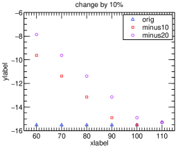
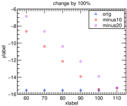
Figure 1: BiCGstab solver residual $r$ for the solution of the free Wilson Dirac propagator on a $12^{3}\times T$-lattice with $T=\{60,70,80,90,100,110\}$ after convergence (triangles) and after having changed the solution on the last 10 time slices (squares) and on the last 20 time slices (circles) by $+10\%$ and $+100\%$ respectively.

We illustrate the problem with a numerical study in the QCD Schrödinger Functional using the double precision version of the MILC code [15]. The parameters were $am\simeq 0.5$ ($\kappa=0.{111111}$), $L/a=12$, and $T/a=\{60,70,80,90,100,110\}$ ($a=1$ in the following) and we used a unit gauge background. Using the stabilised bi-conjugate gradient algorithm (BiCGstab) [16], we solved $D\psi=\eta$ for $\psi$, which corresponds to a column of the quark propagator. As is common practise, we used $r\leq 10^{-15}$ for the stopping criterion.

As a test of the solver residual and of proper convergence for large $t$, we changed the solution $\psi(t,\vec{x})$ by +10% (or +100%), once for $t\geq T-10$ and once for $t\geq T-20$ for all the values of $T$ mentioned above and then recomputed $r$. Figure 1 shows the results. The triangles represent the achieved solver residual for each choice of $T$ and the squares and circles represent the residual $r$ after having changed the solution for $t\geq T-10$ and $t\geq T-20$, respectively. We see that above a certain time-extent $T$ of O($100$) the residual ceases to be sensitive to a change of the solution by 10% (or 100%). In this situation the computed solution $\psi$ cannot be considered correct.

3 The 1-dimensional Dirac operator

The problem we observed in 4 dimensions is also present in 1-dimension. To illustrate this we implemented the equation $D\psi=\eta$ in MATLAB with $D$ given by the 1-dimensional free Wilson lattice Dirac operator with periodic boundary conditions,

$$D^{(1)}_{xy}\equiv\delta_{xy}-\kappa\left[\delta_{y,x+1}(1+\gamma_{1})+\delta_{y,x-1}(1-\gamma_{1})\right],$$ (4)

where $\kappa=1/(2m+2)$ is the hopping parameter. We solved for $\psi$ using a stabilised BiCG algorithm in double precision. Since we implemented the Dirac equation on the torus, we expect the problem to appear at around twice the time extent observed in the Schrödinger functional. Indeed, for $T=180,\;m=0.5$ and $r=10^{-15}$ the solution vector varies in time by more orders of magnitude than can be represented by the arithmetic precision and vanishes exactly for the 10 central lattice points. One therefore expects the solution to be wrong for a time interval larger than 10 time slices around $T/2$.

4 The (multiplicative) Schwarz alternating procedure (SAP)

We now give our proposal to circumvent the problem. We decompose the time-direction of the lattice into a number of domains, such that the solution is expected to decay by fewer orders of magnitude than covered by the arithmetic precision within each domain.

We adopt the notation given by Lüscher [12] and briefly review some basic definitions. We decompose the problem into $n_{\rm dom}$ non-overlapping domains. Each domain $\Lambda$ has an interior boundary $\partial\Lambda^{\ast}$ and an exterior boundary $\partial\Lambda$ (cf. figure 2).

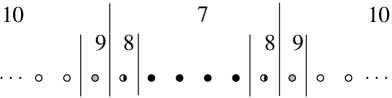
Figure 2: Domain of size $L_{1}=6$. The black dots represent the bulk of the domain $\Lambda$, the interior boundary $\partial\Lambda^{\ast}$ is represented by the half-filled dots and the exterior boundary $\partial\Lambda$ is represented by the grey circles. The complement of $\Lambda$ is $\Lambda^{\ast}$.

The position-space Dirac operator may be written in the form

$$D=\left(\begin{array}[]{ll}D_{\Lambda}&D_{\partial\Lambda}\\ D_{\partial\Lambda^{\ast}}&D_{\Lambda^{\ast}}\\ \end{array}\right),$$ (5)

where the matrices $D_{\Lambda}$ and $D_{\Lambda^{\ast}}$ act on the domain $\Lambda$ and its complement $\Lambda^{\ast}$, respectively. The off-diagonal matrices $D_{\partial\Lambda}$ and $D_{\partial\Lambda^{\ast}}$ contain those interactions that couple $\Lambda$ to the adjacent domains.

Following [12], the algorithm we propose visits each of the $n_{\rm dom}$ domains in successive sweeps and updates the current approximation $\psi$ to the solution of $D\psi=\eta$ according to

$$\psi^{\prime}=\psi+D_{\Lambda}^{-1}(\eta-D\psi).$$ (6)

Here we take $\psi=0$ as the initial guess. We introduce the domain based stopping criterion

$$r_{\rm dom}=\max\limits_{\Lambda}\left\{{\sqrt{|D\psi-\eta|^{2}_{\Lambda}/|\psi|_{\Lambda}^{2}}}\right\}\leq 10^{-15}.$$ (7)

Note that we normalise with respect to the solution vector since one usually uses a $\delta$-function as source $\eta$.

5 Numerical results

We first computed $\psi$ on the whole lattice in 1 dimension by means of Fourier transformation in Mathematica. Since this software allows for arbitrary numerical precision we could thereby obtain an exact reference solution. We then implemented the SAP solver in MATLAB, where all further numerical tests have been performed. Within each sub-domain the current update for the solution $\psi$ is computed using a BiCG solver which runs until convergence. As an example we discuss the case $T=120$ and $m=0.5$. The SAP solver takes about 10 times more iterations than the conventional (unreliable) BiCG with a global stopping criterion like in eq. (3). Notice that the matrix $\times$ vector operations needed in the SAP solver clearly involve smaller matrices. However, for heavy quarks the condition number of the Dirac matrix is not very large and the main issue is rather the precision. The results for both algorithms are illustrated in figure 3 in terms of the time-slice relative error with respect to the exact solution. Two comments are in order :

• Without domain decomposition the solution $\psi$ deviates strongly from the exact solution despite alleged proper convergence of the solver indicated by the residual $r$.

• The circles in fig. 3 show the relative error for the solution computed with the method suggested in this work. Notably it stays at the desired level over the whole time extent of the lattice, indicating uniform convergence.

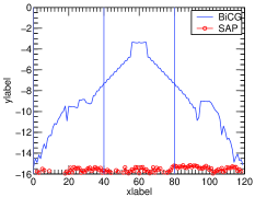
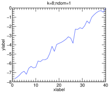
Figure 3: Left: Example of solver accuracy for $n_{\rm dom}=3,m=0.5$ and $T=120$ (vertical lines indicate the domain-borders). The blue lines (red circles) represent the relative error of the result obtained by the BiCG (SAP) solver with respect to the exact solution. Right: Time-slice residual for the problem $D_{\Lambda}^{-1}(\eta-D\psi)=\delta$ after the 8th sweep of the SAP solver over the 1st domain ($T=120$).

6 Conclusions

We have given numerical evidence that conventional CG-solvers run into round-off problems when the lattice volume and the quark mass are large. In particular the solver residual $r$ given in eq. (3) is misleading in these cases. We have performed preliminary tests of an algorithm and a residual based on the Schwarz alternating procedure that do not suffer from these problems.

In contrast to the conventional solver, the algorithm we suggest converges to a constant precision over the whole lattice. Still one might expect the local residual to grow within each domain. This is indeed visible when the problem $D_{\Lambda}^{-1}(\eta-D\psi)=\delta$ is considered (see figure 3, right plot).

The parameter range where the algorithm applies is complementary to that for conventional CG-solvers for small quark masses on the one hand and to that for the procedure based on the hopping parameter expansion for very large quark masses [17] on the other hand. The algorithm suggested here should in fact allow a more precise assessment of the range of quark masses where the latter method is applicable.

The implementation in 4 dimensions should be straightforward. In QCD a gain in performance could presumably be achieved by starting with the free propagator as initial guess. It would be very interesting to investigate the influence of overlapping domains on the solver performance.

Acknowledgements: We warmly thank Jonathan Flynn and Ulli Wolff for their helpful comments and for reading the manuscript. This work was supported by the SFB/TR 09 of the Deutsche Forschungsgesellschaft and the PPARC grant PPA/G/O/2002/00468.

References

- [1] P. Boyle et al., The QCDOC project, Nucl. Phys. Proc. Suppl. 140 (2005) 169–175, [hep-lat/0110197].
- [2] F. Bodin et al., The APEnext project, Nucl. Phys. Proc. Suppl. 106 (2002) 173–176, [hep-lat/0110197].
- [3] A. Ukawa, The PACS-CS project, In these proceedings.
- [4] A. Jüttner, Precision lattice computations in the heavy quark sector, PhD Thesis [hep-lat/0503040].
- [5] ALPHA Collaboration, J. Rolf et al., Towards a precision computation of in quenched QCD, Nucl. Phys. Proc. Suppl. 129 (2004) 322–324, [hep-lat/0309072].
- [6] E. Eichten and B. Hill, An effective field theory for the calculation of matrix elements involving heavy quarks, Phys. Lett. B234 (1990) 511.
- [7] A. X. El-Khadra, A. S. Kronfeld, and P. B. Mackenzie, Massive fermions in lattice gauge theory, Phys. Rev. D55 (1997) 3933–3957, [hep-lat/9604004].
- [8] S. Aoki, Y. Kuramashi, and S. Tominaga, Relativistic heavy quarks on the lattice, Prog. Theor. Phys. 109 (2003) 383–413, [hep-lat/0107009].
- [9] H. A. Schwarz, Gesammelte Mathematische Abhandlungen, vol. 2 (Springer Verlag, Berlin, 1890).
-
[10]
Y. Saad, Iterative methods for sparse linear systems, 2nd ed. (SIAM,
Philadelphia, 2003); see also
http://www-users.cs.umn.edu/~saad/. - [11] S. Sint, On the Schrödinger Functional in QCD, Nucl. Phys. B421 (1994) 135–158, [hep-lat/9312079].
- [12] M. Lüscher, Solution of the Dirac equation in lattice QCD using a domain decomposition method, Comput. Phys. Commun. 156 (2004) 209–220, [hep-lat/0310048].
- [13] M. Lüscher, Lattice QCD and the Schwarz alternating procedure, JHEP 05 (2003) 052, [hep-lat/0304007].
- [14] M. Lüscher, Schwarz-preconditioned HMC algorithm for two-flavour lattice QCD, [hep-lat/0409106].
-
[15]
“MIMD Lattice Computation (MILC) Collaboration, homepage
http://physics.indiana.edu/~sg/milc.html.” - [16] A. Frommer, V. Hannemann, B. Nockel, T. Lippert, and K. Schilling, Accelerating Wilson fermion matrix inversions by means of the stabilized biconjugate gradient algorithm, Int. J. Mod. Phys. C5 (1994) 1073–1088, [hep-lat/9404013].
- [17] B. A. Thacker and G. P. Lepage, Heavy quark bound states in lattice QCD, Phys. Rev. D43 (1991) 196–208.