In search of a Hagedorn transition in
$SU(N)$ lattice gauge theories at large–$N$

Abstract

We investigate on the lattice the metastable confined phase above $T_{c}$ in $SU(N)$ gauge theories, for $N=8,10$, and $12$. In particular we focus on the decrease with the temperature of the mass of the lightest state that couples to Polyakov loops. We find that at $T=T_{c}$ the corresponding effective string tension $\sigma_{\text{eff}}(T)$ is approximately half its value at $T=0$, and that as we increase $T$ beyond $T_{c}$, while remaining in the confined phase, $\sigma_{\text{eff}}(T)$ continues to decrease. We extrapolate $\sigma_{\text{eff}}(T)$ to even higher temperatures, and interpret the temperature where it vanishes as the Hagedorn temperature $T_{H}$. For $SU(12)$ we find that $T_{H}/T_{c}=1.116(9)$, when we use the exponent of the three-dimensional XY model for the extrapolation, which seems to be slightly preferred over a mean-field exponent by our data.

I Introduction

In the large–$N$ limit the confined phase of the $SU(N)$ gauge theory becomes weakly interacting and relatively simpler ’t Hooft (1974); Witten (1979). Moreover, some of its features can be described by a low energy effective string theory (for example see Polchinski (1992)). The link between gauge theories and string theories was strengthened with the conjectured AdS/CFT dualities between supersymmetric Yang-Mills theories in the large–$N$ limit and gravity models (for a review see Aharony et al. (2000)). An interesting element of systems with stringy properties is the occurrence of an ultimate temperature, above which the free string description is unsuitable. In string models for QCD (or pure gauge theory), this temperature is naturally identified with a ‘Hagedorn’ deconfinement transition.

The earliest evidence for the existence of a finite temperature phase transition in hadronic physics was obtained by Hagedorn in Hagedorn (1965). There, he assumed that hadronic states with mass $m\to\infty$, referred to as “fireballs”, are compound systems of other fireballs. This can be stated mathematically by a self-consistent relation that the density of states $\rho(E)$ must obey, and that results in an exponential growth of $\rho$ with the energy $E$. An immediate consequence is that there exists a temperature $T_{H}$, above which the partition function diverges: as $T\to T_{H}^{-}$, the Boltzmann suppression of states $\propto\exp(-E/T)$ is overwhelmed by the density of states, $\rho(E)\propto\exp(+cE)$. At this $T$ an increase of the system’s energy is met with an increase in the number of particles. In the bootstrap dynamical framework, which predated the discovery of QCD and the idea that hadrons are confined bound states of quarks and gluons, $T_{H}$ represents an ultimate temperature beyond which matter cannot be heated. In the more appropriate language of QCD, once we are close enough to $T_{H}$ for these fireballs to be densely packed, the underlying quark and gluon degrees become liberated from their ‘hadronic bags’ and we expect to see a deconfinement transition Cabibbo and Parisi (1975).

A simple, intuitive, and general analogue of the above argument Polyakov (1978); Banks and Rabinovici (1979) in the context of any linearly confining theory is as follows. In such a theory the energy of a string of length $l$ between two distant static sources a distance $r<l$ apart, obeys

$$E(l;r)\simeq\sigma l,$$ (1)

where $\sigma$ is the confining string tension and we neglect subleading terms. For a string (or for a long enough flux tube) it is easy to see that once $l\gg r$ the number of different states of the string grows exponentially with $l$, $n(l)\propto\exp(cl)$, up to power factors, with $c$ determined by the dynamics and dimensionality. On the other hand the probability of such a string with $l\gg r$ is suppressed by a Boltzmann factor, $\propto\exp(-E(l)/T)$. The total probability of such a string is given by the free energy that combines the two factors to define an effective string tension $\sigma_{\rm eff}(T)$:

$$\propto\exp{\left[\left(c-\sigma/T\right)\cdot l\right]}\equiv\exp\left(-\sigma_{{\rm eff}}(T)l/T\right).$$ (2)

It is thus clear that as $T\to T_{H}\equiv\sigma/c$, arbitrarily long loops will be thermally excited and the effective string tension vanishes, $\sigma_{{\rm eff}}\stackrel{{\scriptstyle T\to T_{H}}}{{\longrightarrow}}0$. Because of this vanishing energy, and other features of the free energy Cabibbo and Parisi (1975), one would naturally expect this deconfining phase transition to be second order.

We can give a parallel argument for the partition function itself. Consider an $SU(N)$ gauge theory in which the confining energy eigenstates are composed of glueballs. A model for glueballs is to construct them from closed loops of (fundamental) flux. For the lightest glueballs this loop will be small, and given that the width of the flux tube is $O(1/\surd\sigma)$, it does not make much sense to think of a distinct closed loop of flux. However in the sector of highly excited glueballs, the loop will be very long and the presence of such states becomes compelling. For a state composed of a flux loop of length $l$, the energy is $E\sim\sigma l$. What is the number density, $n_{G}(E)$, of such states? Such highly excited states have large quantum numbers and in this limit a classical counting of states is justified. Thus the number of these states equals the number of closed loops of length $l$, i.e. $n_{G}(E)\propto\exp(cl)$ up to subleading factors, with the scale $c$ identical to the one in Eq. (2). Thus the partition function will have a Hagedorn divergence as $T\to T_{H}$ where $T_{H}$ is identical to the string condensation temperature of the previous paragraph.

Since we expect $c\sim\surd\sigma$, we expect the Hagedorn transition to occur at $T_{H}=\sigma/c\sim\surd\sigma$. On the other hand the lightest glueball (a scalar) satisfies $m_{G}\simeq 3.5\surd\sigma$ while the next lightest glueball (a tensor) satisfies $m_{G}\simeq 4.8\surd\sigma$. Thus one has the somewhat counterintuitive picture that as $T\to T_{H}$ the lightest glueballs are not thermally excited. Rather it is the highly excited glueballs, whose density of states grows exponentially with their mass, that drive the transition.

In the above scenarios, as $T\to T_{H}$ the vacuum becomes increasingly densely packed with the thermally excited states. These will at some point start to interact and the idealised arguments we use necessarily break down as $T$ approaches $T_{H}$. We note that as $N\to\infty$ for $SU(N)$ gauge theories (or QCD), interactions between colour singlet states vanish. Thus it is in this limit that the argument for a Hagedorn transition becomes most compelling.

The vanishing of $\sigma_{\rm eff}$, and the divergence of the associated correlation length, suggests that this Hagedorn transition is second order. To what universality class might it belong? The high temperature phase has a nonzero vacuum expectation value for the complex valued Polyakov lines that wind around the Euclidean temporal torus. This spontaneously breaks the global $Z_{N}$ symmetry of the theory. Using universality arguments one can then predict the critical exponents of the transition Svetitsky and Yaffe (1982). In particular, in three spatial dimensions it belongs to the universality classes of the three-dimensional Ising and XY models for $N=2$ and $N\geq 4$ (for $N=3$, there is no known universality class) Svetitsky (1986). Finally for $N=\infty$ there are studies that predict mean-field behaviour for the correlation length Dumitru et al. (2005). This can be understood as a suppression of the critical region by powers of $1/N$ (see for example the discussion in Bringoltz (2005), and references therein). The study in Aharony et al. (2004) also gives mean-field scaling, however only because infrared divergences are not seen at the small volume discussed there Aharony (2005).

The above discussion has so far ignored the contribution to the partition function that comes from nonconfined energy eigenstates containing a finite density of gluons. While such states will be irrelevant at low $T$, the fact that their entropy grows as $N^{2}$ while the entropy of confined states is at most weakly dependent on $N$, means that for large enough $N$ there must be some $T$ where their free energy will decrease below that of the confined sector of states. At this point there will be a phase transition to a (perhaps strongly interacting) ‘gluon plasma’, which one would naturally expect to be first order. Indeed it turns out to be the case that in four dimensions $SU(N)$ gauge theories go through a first order deconfining transition for $N\geq 3$ Lucini et al. (2004). (See also the latent heat calculation at large-$N$ on a symmetric lattice Kiskis (2005).) For SU(2) the transition is second order, but it is not clear if it is a Hagedorn transition. The fact that it is at small rather than large $N$ makes the case weaker. As does the fact that the $SU(2)$ value of $T_{c}/\surd\sigma$ lies on the curve that interpolates through the $N\geq 3$ values Lucini et al. (2004). On the other hand the value of $T_{c}/\surd\sigma$ does coincide with the string condensation temperature of the simple Nambu-Goto string theory (see below).

The fact that for $N\geq 3$ the first order deconfining transition occurs for $T_{c}<T_{H}$, would appear to render the Hagedorn transition inaccessible. However the deconfining transition is strongly first order at larger $N$, and so one can try to use its metastability to carry out calculations in the confining phase for $T>T_{c}$. If $T_{H}$ is not far away, one can then hope to calculate $\sigma_{\text{eff}}(T)$ over a range of $T$ where it decreases sufficiently that an extrapolation to $\sigma_{\text{eff}}(T_{H})=0$ can be attempted. In the range of $N$ accessible to us, the interface tension between confined and deconfined phases increases with $N$ faster than the latent heat, and this makes the metastability region larger Lucini et al. (2005) as $N$ grows. Thus such a strategy has some chance of success, and it is what we shall attempt in this paper.

Our strategy is therefore to begin deep enough in the confined phase and then to increase the temperature to temperatures $T>T_{c}$, calculating the decrease in $\sigma_{\rm eff}(T)$, and extrapolating to $\sigma_{\rm eff}=0$. We interpret the result of the extrapolation as the Hagedorn temperature, $T_{H}$. Nevertheless, since we work with finite values of $N$ and volume $V$, tunneling probably occurs somewhere below $T_{H}$. These tunneling effects and the fact that as $\sigma_{\rm eff}$ decreases finite volume effects become important, can make an apriori fit for the functional form of $\sigma_{\rm eff}(T)$ unreliable. As a result we first perform fits where we fix the functional behaviour to be

$$m\equiv\sigma_{\text{eff}}/T\stackrel{{{}_{T\to T_{H}}}}{{{}_{\sim}}}\left(T_{H}/T_{c}-T/T_{c}\right)^{\nu}.$$ (3)

where $\nu=0.6715(3)$ corresponding to 3D XY Pelissetto and Vicari (2002) or $\nu=0.5$ corresponding to mean field. The reason for these two choices is motivated by two conceivable ways in which the low energy effective loop potential can behave (see below). In addition we also perform fits where the exponent $\nu$ is a free parameter, constrained to the range $[0,1]$, and find it to be especially useful for $SU(12)$. The coefficient $A$ is fitted as well. An additional outcome of this work is to confirm that at $T=T_{c}$ the mass of the timelike flux loop that couples to Polyakov loops is far from zero at large-$N$, which confirms that the transition is strongly first-order. To make this point clear we will present figures of the effective string tension in units of the zero temperature string tension $\sigma$. As a function of $T$, it should have the following behavior.

$$\sigma_{\text{eff}}/\sigma\stackrel{{\scriptstyle T\to T_{H}}}{{{}_{=}}}A\cdot T/T_{c}\cdot\left(T_{H}/T_{c}-T/T_{c}\right)^{\nu},$$ (4)

If we imagine the effective potential for an order parameter such as the Polyakov loop, $V_{\text{eff}}(l_{p})$, then at $T=T_{c}$ this will possess degenerate minima corresponding to the confined and deconfined phases. These will be separated by a barrier whose height is expected to be $O(N^{2})$ at large $N$. As we increase $T$ the confined minimum rises relative to the deconfined one(s). As $T\to T_{H}$ we expect the second derivative at the confining minimum to go to zero, corresponding to $\sigma_{\text{eff}}\to 0$. The simplest possibility is that at this $T$ the confining minimum completely disappears, i.e. that this corresponds to a spinodal point of the potential. In a string model of glueballs where the glueball is composed of two ‘constituent’ gluons joined by an adjoint flux tube, string condensation would correspond to the explicit release of a gluon plasma simultaneously throughout space and the identification of the Hagedorn transition with a spinodal point would be compelling. This is less clear in the closed flux loop model. (Whether the increasing stability of the adjoint string as $N\to\infty$ allows us to use the adjoint string model for the highly excited states relevant near $T_{H}$ also needs consideration.) If this Hagedorn transition-spinodal point identification is indeed correct, then in the vicinity of $l_{p}\simeq 0$, the effective loop potential looks like that of a Gaussian model, and $\nu=0.5$ is expected. A model for this behaviour is in Aharony et al. (2004), where because of the infinitesimal volume, any infra-red divergences are excluded, and one has mean-field scaling close to $T_{H}$, which also implies $\nu=0.5$.

In principle it seems quite possible that $T_{H}$ does not coincide with the spinodal transition temperature, $T_{s}$. The temperature $T_{H}$ is a natural concept if one has a good description of the confined phase as an effective string theory. The latter will have $O(1/N)$ interactions, and thus to leading order, lead to a Hagedorn behaviour at a certain temperature $T_{H}$. On the contrary, $T_{s}$ most probably encodes information on the gluonic deconfined phase, which might not be contained in the string theory. Without any other information in the spirit of the calculations Aharony et al. (2004), that identifies $T_{H}=T_{s}$, these two temperatures may be different.

If $T_{H}<T_{s}$ then our method for identifying $T_{H}$ remains valid. In that case one may write down a Landau-Ginzburg theory that has a second order Hagedorn transition at $T_{H}$, from the confined vacuum, $C$, to a deconfined one, $D_{1}$. This happens at $T_{H}>T_{c}$, where both $C,D_{1}$ are metastable, and another deconfined vacuum $D_{2}$ is stable. At large-$N$, the metastability may be strong enough such that this embedded second order phase transition happens without being sensitive to tunnelings into the real vacuum. In this case, the fixed point that controls the critical behavior of the transition is that of the 3D XY model. Nonetheless, to see this nontrivial critical behavior one must be very close to $T_{H}$. This happens because interactions between the Polyakov loops are $O(1/N^{2})$ suppressed, and taking the $N=\infty$ limit before $T\to T_{H}$ results in a Gaussian model and to $\nu=0.5$. To see the scaling behavior of the 3DXY model, one needs to take $T\to T_{H}$ together with $N\to\infty$. In other words, the critical region of this second order transition has a width that shrinks with increasing $N$ Bringoltz (2005). To see this we can examine the renormalization of the $\lambda|l_{p}|^{4}$ interaction in the Landau-Ginzburg-Wilson effective action of the transition. As usual, $\lambda$ gets renormalized by infra-red (IR) modes, and in three spatial dimensions it gets a contribution of $O(\lambda^{2}/m)$. Since $\lambda\sim 1/N^{2}$, this becomes significant only if $m\sim 1/N^{2}$. Using $m^{2}\sim(T_{H}-T)$, this means that the IR modes drive the system to the 3DXY universality class only if $(T_{H}-T)\stackrel{{\scriptstyle<}}{{{}_{\sim}}}1/N^{4}$. Outside of this regime the correlation length has the MF scaling $\nu=0.5$.

Finally, in the case of $T_{H}>T_{s}$ then the spinodal transition may (but need not) interfere with our determination of $T_{H}$. This is a significant ambiguity that we cannot resolve in the present calculations but the reader should be aware of its existence.

We finish by listing some of the reasons that motivate our study. First it gives nonperturbative information about the free energy as a function of the Polyakov loop. While the value of $T_{c}$ tells us when the ordered and disordered minima have the same free energy, the function $\sigma_{\rm eff}(T)$ indicates how the curvature of the free energy at the confining vacuum changes with $T$ and its vanishing may indicate the point at which the confining vacuum becomes completely unstable. This information can serve to constrain the form of the potential in effective models for the Polyakov loops (like those in Dumitru et al. (2005), for example). Second, this study is a first attempt to investigate the validity of nonzero temperature mean-field theory techniques of large–$N$ lattice gauge theories in the continuum. A related study Chandrasekharan and Strouthos (2005) in the strong-coupling limit saw that mean-field theory predictions at finite temperature are simply incorrect, which is consistent with the fact that the large–$N$ limit of these strongly-coupled fermionic systems is mapped to classical systems at finite temperature, whose universality class is not mean-field Bringoltz (2005). It is of prime interest to know if the same happens in the continuum limit of the pure gauge theory, which we are much closer to. The Hagedorn temperature $T_{H}$ can also give an estimate of the central charge of a possible underlying string theory Meyer and Teper (2004), and finally it is interesting to know what is the limit of $T_{H}/T_{c}$ when $N\to\infty$. This limit should be larger than $1$, given that the deconfining phase transition has been shown to be first order at $3\leq N\leq 8$ Lucini et al. (2004). It is however possible that $T_{H}/T_{c}$ is close to $1$ and perhaps decreasing with $N$ which opens up interesting new possibilities in the $N=\infty$ limit.

II Lattice calculation

We work on a lattice with $L^{3}_{s}\times L_{t}$ sites, where $L_{t}$ is the lattice extent in the Euclidean time direction. The partition function is give by

$$Z=\int DU\exp{\left(-S_{\rm W}\right)},$$ (5)

where $S_{\rm W}$ is the Wilson action given by

$$S_{\rm W}=\beta\sum_{P}\left[1-\frac{1}{N}{\rm Re}\text{Tr}\,{U_{P}}\right].$$ (6)

Here $\beta=2N^{2}/\lambda$, and $\lambda=g^{2}N$ is the ’t Hooft coupling, kept fixed in the large–$N$ limit. $P$ is a lattice plaquette index, and $U_{P}$ is the plaquette variable given by multiplying link variables along the circumference of a fundamental plaquette. Simulations are done using the Kennedy-Pendleton heat bath algorithm for the link updates, followed by five over-relaxations. We focus on the measurement of the correlations of Polyakov lines, which are taken every five sweeps.

The Monte-carlo simulations were done using two different methods, which for convenience we refer to as method “A” and method “B”. In both, the calculation was initialized with a field configuration at the lowest value of $\beta$ which was preceded by at least $3000$ thermalization sweeps from a cold start. Then, in method B, to reduce thermalization effects, each value of $\beta$ was simulated beginning from the previous one. In contrast, in method A, more than one simulation began from the same $\beta$. This serves to eliminate the dependence between different simulations. We choose to use method $A$ and method $B$ for $N=8$ and $N=12$ respectively. In the case of $N=10$ we used both methods, and could compare between them. In Tables 1-2, where we present results obtained with method A, we give the initial configurations for each value of $\beta$, along with the statistics of the study. The number of thermalization sweeps for $N=8,10$ for each value of $\beta$ was always at least $3000$. As mentioned, the $SU(12)$ calculations were done with method B, and less thermalization sweeps (at least $400$) were needed for each value of $\beta$. For each data set, we calculate the correlation functions of the thermal lines with improved operators Lucini et al. (2005), and use a variational technique to extract the lightest masses Wilson (March 1981); Falcioni et al. (1982); Ishikawa et al. (1982); Berg et al. (1982); Luscher and Wolff (1990), the results for which are given in lattice units, $am$, in Tables 1-4, where the errors are evaluated by a jack-knife procedure.

To check that the results of method A are properly thermalized we also calculate the masses by excluding an additional $3000$ sweeps (in addition to the standard thermalization sweeps). This results in a new set of masses, which we refer to as $am_{\rm hot}$, and which we present in Tables 1–2. We find that in general the thermalization effects are not significant, and in almost all cases $am_{\rm hot}$ agrees with $am$ to within one sigma.

The physical scale $a\surd\sigma$ listed in the Tables was fixed using the interpolation for the string tension given in Lucini et al. (2005) in the case of $SU(8)$. For $N=10,12$ we extrapolate the parameters of the scaling function of Lucini et al. (2005), $c_{0,1,2}$, and $\beta_{0}/N^{2}$, in $1/N^{2}$ from their values at $N=6,8$. In addition we measured the string tension for $N=10$ at $\beta=68.80$ on an $8^{4}$ lattice, and for $N=12$ at $\beta=99.2,100.0$, on an $8^{4}$, and a $10^{4}$ lattice respectively. The results, together with the string tensions calculated with the scaling function, are given in Table 5. We find that assuming an error only in the measured string tension, then the measured and calculated string tensions deviate at most by $1.6\sigma$. Evaluating the extrapolation error will make the agreement better.

Let us note here that the points used for the fits exclude values of $\beta$ in which tunneling to the deconfined phase was observed. Tunnellings were identified by observing double peaks in the histogram of the expectation values of the Polyakov lines, and by identifying clear tunneling configurations (again using the Polyakov lines as a criterion). For other values of $\beta$, we observe an increase in the fluctuations of the lines with $T$, but did not see any tunneling configurations. Correspondingly, the histograms widen with $T$, and for some values of $\beta$ start to develop asymmetric tails. Nevertheless in all these cases the overall average of the bare Polyakov line was always lower than $3\times 10^{-3}$. The $\beta$ values of the excluded deconfining simulations are $\beta=44.01,44.015$ for $SU(8)$, and $\beta=69.10,69.14,69.16$, and $69.17$ for $SU(10)$ (for method A), as noted in Tables 1–2. For the case of $SU(12)$ the last point of $\beta=99.95$ was still confining after $10,000$ sweeps. At the next value of $\beta=100.00$ the $12^{3}\times 5$ system already showed signs of instability.

Finally, to check the effect of finite volume corrections, which potentially increase as the mass decreases towards $T_{H}$, we perform several additional calculations of the correlation lengths. In the case of $N=12$ we performed a single calculation on a $16^{3}\times 5$ lattice at the smallest volume with $\beta=99.95$. The mass obtained after 5,000 thermalization sweeps and 10,000 measurement sweeps, is $am=0.187(14)$, and agrees very well with the result obtained on the $12^{3}\times 5$ lattice (both are presented in Table 4). For $N=10$ in method B, all values of $\beta$ were simulated on both a $12^{3}\times 5$ lattice, and a $14^{3}\times 5$ lattice. The results are presented in Table 3, and we find at most a $1.3\sigma$ difference between them. Comparing with the situation close to the second order phase transition of the $SU(2)$ group Lucini et al. (2005), we find that for $N=2$, finite volume effects are much more important than for $N=12$. This puts the results of this work, which were largely done for only one lattice volume, on a more solid footing. This is also consistent with standard theoretical arguments that predict smaller volume corrections for gauge theories with larger values of $N$.

Table 1: Statistics and results of the Monte-Carlo simulations for $N=8$, obtained with method A. The “D” denotes tunneling to deconfining configurations, which is not considered for the fits. $am_{\text{ hot}}$ is the result of the data set that excludes the first 3000 measurement sweeps.

$N=8$
$\beta$	$am$	$am_{\text{ hot}}$	$a\sqrt{\sigma}$	Initial	(no. of sweeps)$/10^{3}$
	(all sweeps)
43.850	0.361(17)	0.362(17)	0.3615	Frozen	20.0
43.875	0.336(22)	0.362(22)	0.3580	43.850	15.0
43.900	0.334(17)	0.337(17)	0.3547	43.875	13.0
43.930	0.272(19)	0.270(19)	0.3507	43.875	17.0
43.950	0.314(15)	0.326(15)	0.3481	43.850	24.0
43.975	0.286(17)	0.283(17)	0.3448	43.950	10.0
43.980	0.258(18)	0.245(18)	0.3442	43.975	13.0
43.985	0.304(14)	0.294(14)	0.3436	43.975	13.0
43.995	0.206(13)	0.207(13)	0.3423	43.975	14.0
44.000	0.264(17)	0.260(17)	0.3417	43.850	29.0
44.01;D	-	-	0.3404	44.000	13.0
44.015;D	-	-	0.3398	44.000	13.0
44.020	0.240(17)	0.253(17)	0.3392	44.000	15.0
44.025	0.228(17)	0.201(17)	0.3385	44.000	16.0
44.033	0.213(14)	0.220(14)	0.3376	44.000	20.0

Table 2: Results and statistics of the Monte-Carlo simulations for $N=10$ obtained with method A. The “D” denotes tunneling to deconfining configurations. $am_{\rm hot}$ are the results of the data set that excludes the first 3000 measurement sweeps.

$N=10$
$\beta$	$am$	$am_{\text{hot}}$	$a\sqrt{\sigma}$	Initial	(no. of
	(all sweeps)			config.	sweeps)/$10^{3}$
68.5000	0.571(41)	0.609(34)	0.3941	frozen	17.0
68.5520	0.524(28)	0.514(29)	0.3888	68.50	22.0
68.6000	0.545(11)	0.544(11)	0.3839	68.50	23.5
68.6553	0.502(13)	0.500(14)	0.3785	68.60	20.5
68.7000	0.481(36)	0.441(35)	0.3742	68.50	23.5
68.7500	0.452(12)	0.453(14)	0.3695	68.50	23.0
68.8000	0.391(17)	0.388(19)	0.3649	68.50	26.0
68.8500	0.389(14)	0.378(22)	0.3603	68.50	24.0
68.9000	0.356(15)	0.345(16)	0.3559	68.50	23.0
68.9500	0.287(15)	0.289(16)	0.3516	68.50	23.5
69.0000	0.295(17)	0.286(17)	0.3473	68.50	25.0
69.0100	0.295(13)	0.294(14)	0.3465	69.00	23.0
69.0200	0.315(15)	0.312(15)	0.3457	69.00	22.0
69.0412	0.277(15)	0.292(16)	0.3439	69.00	22.0
69.0500	0.271(14)	0.273(16)	0.3432	69.00	21.0
69.0700	0.251(18)	0.242(19)	0.3416	69.00	22.0
69.0816	0.262(16)	0.258(17)	0.3406	69.00	22.0
69.1000	-	-	0.3391	68.50	11.0
69.1100	0.253(11)	0.248(11)	0.3383	69.10	22.0
69.1200	0.233(15)	0.226(16)	0.3375	69.10	22.0
69.1300	0.223(15)	0.231(14)	0.3367	69.10	22.0
69.1400	-	-	0.3359	69.10	12.0
69.1500	0.218(12)	0.228(13)	0.3351	69.10	22.0
69.1600	-	-	0.3344	69.15	8.0
69.1700	-	-	0.3336	69.15	8.0
69.1800	0.222(14)	0.225(16)	0.3328	69.15	18.0
69.1900	0.218(12)	0.228(13)	0.3320	69.15	18.0

Table 3: Masses in lattice units and statistics of the Monte-Carlo simulations for $N=10$ obtained with method B on $14^{3}\times 5$, and $12^{3}\times 5$ lattices.

$N=10$
$\beta$	$12^{3}\times 5$	(no. of sweeps)/$10^{3}$	$14^{3}\times 5$	(no. of sweeps)$/10^{3}$	$a\sqrt{\sigma}$
68.50	0.599(30)	20	0.584(35)	20	0.3941
68.70	0.396(17)	22	0.428(29)	22	0.3742
68.85	0.371(27)	20	0.371(18)	20	0.3603
68.95	0.316(16)	“	0.308(11)	“	0.3516
69.07	0.246(12)	“	0.270(15)	“	0.3416
69.13	0.244(17)	“	0.241(14)	18	0.3367
69.17	0.220(10)	“	0.203(15)	16	0.3336
69.20	0.154(11)	22	0.200(21)	8	0.3313
69.23	0.183(19)	15	-	-	0.3290

Table 4: Results and statistics of the Monte-Carlo simulations for $N=12$ obtained with method B. All masses are calculated on a $12^{3}\times 5$ lattice, except for the last row which is for $16^{3}\times 5$ lattice. The number of thermalization sweeps was at least 400 between two successive values of $\beta$, while it was $800$ for the first calculation of $\beta=99.00$.

$N=12$
$\beta$	$am$	$a\sqrt{\sigma}$	(no. of sweeps)$/10^{3}$
99.00	0.573(25)	0.3866	5
99.20	0.472(24)	0.3729	5
99.40	0.396(18)	0.3601	5
99.60	0.333(17)	0.3479	10
99.80	0.259(13)	0.3365	10
99.90	0.203(13)	0.3310	10
99.95	0.190(13)	0.3284	10
99.95	0.187(14)	0.3284	10

Table 5: String tensions for $SU(10)$ and $SU(12)$.

$N,\beta$	Measurement	Results of scaling function (see text)
$N=10,\beta=68.80$	0.3667(80)	0.3649
$N=12,\beta=99.20$	0.3770(26)	0.3729
$N=12,\beta=100.00$	0.3243(23)	0.3257

If we define the effective string tension, $\sigma_{\text{eff}}(T)$, to be the coefficient of the leading linear part of the free energy of two distant fundamental sources, then $\sigma_{\text{eff}}(T)=mT$ where $m$ is the lightest mass that couples to timelike Polyakov loops. Therefore the ratio $\sigma_{\text{eff}}/\sigma$ will be given by

$$\frac{\sigma_{\text{eff}}}{\sigma}=\frac{am(\beta)}{L_{t}\cdot(a\sqrt{\sigma}(\beta))^{2}}.$$ (7)

At each simulated ratio of $\beta$ we estimate $T/T_{c}$ using

$$\frac{T}{T_{c}}=\frac{(a\sqrt{\sigma})_{c}}{a\sqrt{\sigma}(\beta)},$$ (8)

where $(a\sqrt{\sigma})_{c}$ is the value of $a\sqrt{\sigma}$ at $\beta=\beta_{c}$ for $L_{t}=5$, i.e. $5a(\beta_{c})=T^{-1}_{c}$. It is extracted from $T_{c}/\sqrt{\sigma}$, which is 0.5819(41) for $N=8$. (This assumes that $T_{c}/\sqrt{\sigma}$ varies at most very weakly with $a(\beta)$, which is in fact what one observes Lucini et al. (2005).) The corresponding value for $N=10,12$ is found by extrapolating in $1/N^{2}$ according to measured values of $T_{c}/\sqrt{\sigma}(L_{t}=5)$ for $N=4,6,8$ Teper (2005). This gives 0.5758 for $SU(10)$ and 0.5735 for $SU(12)$, with an error of about $1\%$.

In Figs. 1–5 we give the effective string tensions as a function of temperature for the studied gauge groups and various data sets, as explained above. In view of Eq. (4) we choose to present $\sigma_{\text{eff}}/\sigma$. As the relative error of $am$ is roughly 10 times the one on $T_{c}/\sqrt{\sigma}$, we neglect the latter in our error estimate. The fit to the data was done according Eq. (4), either by fixing $\nu=0.6715,0.5$ for the 3D XY and mean-field universality classes, or in some cases by making $\nu$ a free parameter. The fitting results are presented in Table 6.

Table 6: Results of the fits to Eq. (4). The values of $T_{H}/T_{c}$, and $A$ are presented for all fits. In the cases where a fit with $\nu$ as a free parameter was made, then the resulting $\nu$ is presented in the second column. We present the coverage probability contours in the $A-T_{H}/T_{c}$ plane, when appropriate, in Figs. 6–11.

$N$	Universality class	$\frac{T_{H}}{T_{c}}$	$\frac{T_{H}}{\sqrt{\sigma}}$	$A$	central charge	$\frac{\chi^{2}}{{\text{dof}}}$	dof
8	3D XY	1.093	0.636	2.190	1.178	2.84	11
$12^{3}\times 5$	MF	1.066	0.620	1.728	1.237	2.79	11
(method A)	Free, $\nu=1$	1.145	0.666	3.055	1.073	3.19	10
10	3D XY	1.104	0.636	2.328	1.236	1.44	21
$12^{3}\times 5$	MF	1.078	0.621	1.862	1.178	2.07	21
(method A)	Free, $\nu=1$	1.160	0.668	3.132	1.067	1.16	20
10	3D XY	1.108	0.624	2.112	1.169	3.29	7
$12^{3}\times 5$	MF	1.083	0.638	1.681	1.223	3.56	7
(method B)	Free, $\nu=0.79$	1.127	0.649	2.394	1.131	3.94	6
10	3D XY	1.114	0.642	2.102	1.156	0.68	6
$14^{3}\times 5$	MF	1.087	0.626	1.683	1.215	1.00	6
(method B)	Free, $\nu=1$	1.172	0.675	2.815	1.045	0.60	5
12	3D XY	1.116	0.640	2.337	1.162	0.30	5
$12^{3}\times 5$	MF	1.092	0.626	1.858	1.215	0.50	5
(method B)	Free, $\nu=0.69$	1.119	0.642	2.387	1.156	0.37	4

In Figs. 6–11 we present confidence levels in the fit parameters, for the cases where the fit is good. In the case of two parameter fits, we present contours in the $(A,T_{H}/T_{c})$ plane of the $\chi^{2}$ per degree of freedom levels, which correspond to confidence levels of $68.27\%,90\%$, and $99\%$. These confidence levels are then reflected in the error estimates we give in the text.

When we treat $\nu$ as a free fit parameter as well, we present two dimensional projections (e.g. in $\nu-T_{H}/T_{c}$ space) of a volume in the parameter space of $(T_{H}/T_{c},A,\nu)$ that corresponds to the a confidence level of $68.27\%$ and lower. In this case we do not quote in the text any error estimates together with the central values.

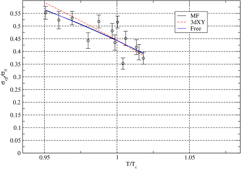
Figure 1: Effective string tension for $SU(8)$ obtained in method A in units of the zero temperature string tension.

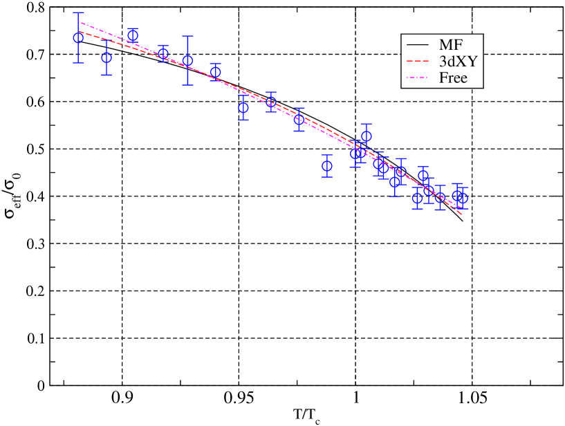
Figure 2: Effective string tension for $SU(10)$ obtained in method A in units of the zero temperature string tension.

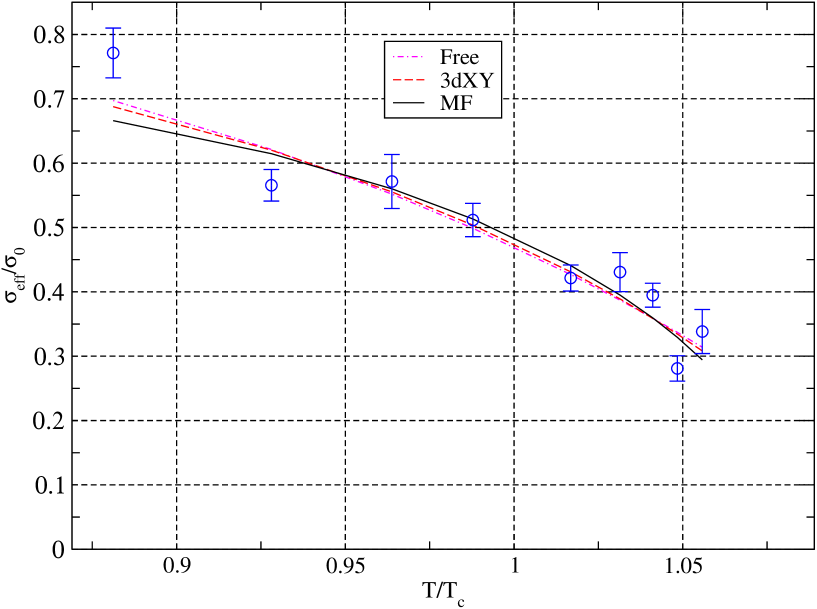
Figure 3: Effective string tension for $SU(10)$ obtained in method B on a $12^{3}\times 5$ lattice, in units of the zero temperature string tension.

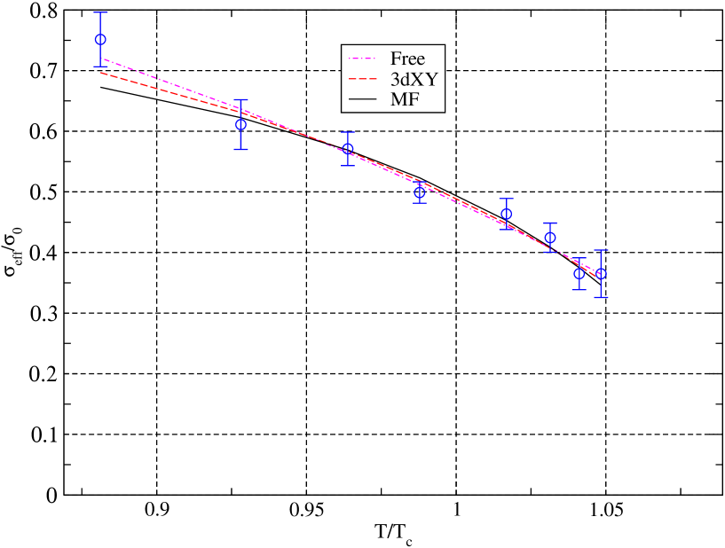
Figure 4: Effective string tension for $SU(10)$ obtained in method B on a $14^{3}\times 5$ lattice, in units of the zero temperature string tension.

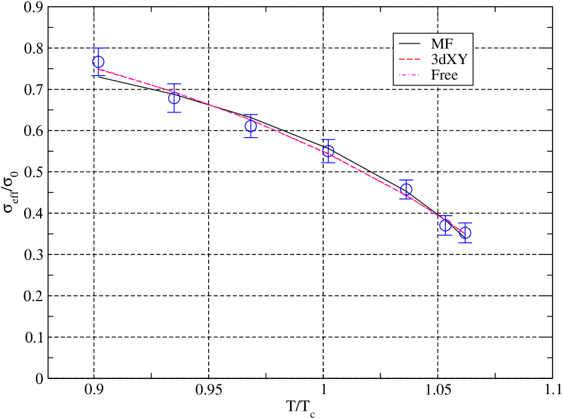
Figure 5: Effective string tension for $SU(12)$ obtained in method B in units of the zero temperature string tension.

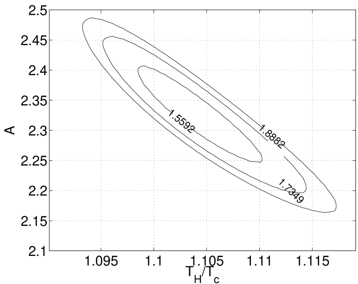
Figure 6: Confidence levels for the fits of $SU(10)$ on a $12^{3}\times 5$ obtained with method A for the 3DXY exponent.

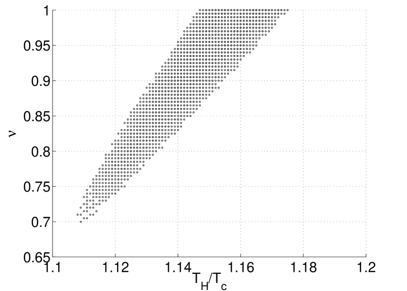
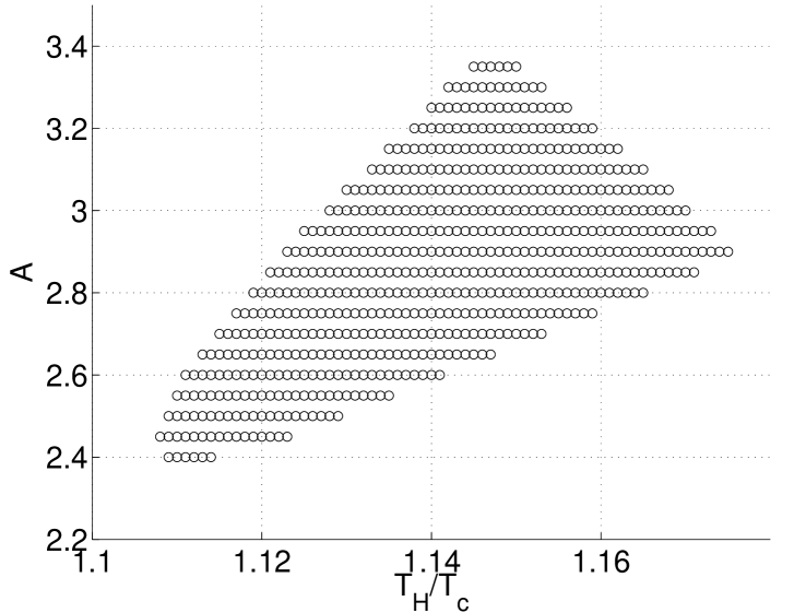
Figure 7: Two dimensional projections of a isosurface in the three-dimensional space of $(\nu,T_{H}/T_{c},A)$ which represents a confidence level of $68.27\%$ for the fits of $SU(10)$ obtained with method A on a $12^{3}\times 5$ lattice, with a free exponent.

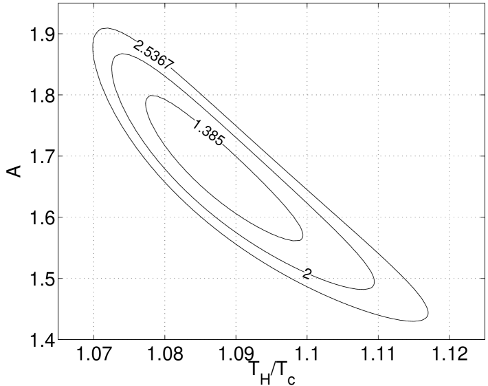
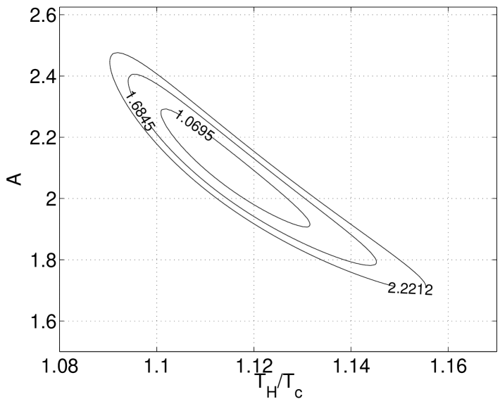
Figure 8: Confidence levels for the fits of $SU(10)$ on a $14^{3}\times 5$ obtained with method B. The plot on the right(left) is for the 3DXY(MF) exponent.

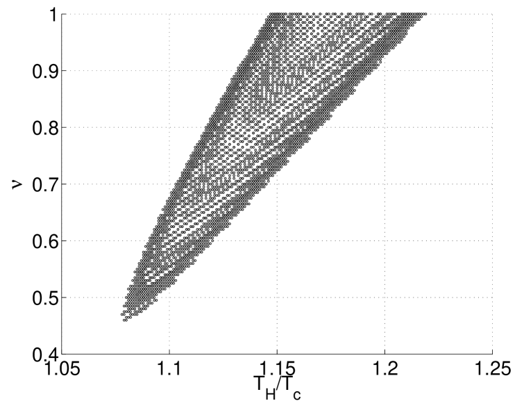
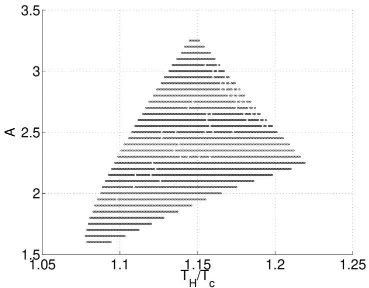
Figure 9: Two dimensional projections of a isosurface in the three-dimensional space of $(\nu,T_{H}/T_{c},A)$ which represents a confidence level of $68.27\%$ for the fits of $SU(10)$ obtained with method B on a $14^{3}\times 5$ lattice, with a free exponent.

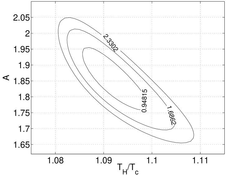
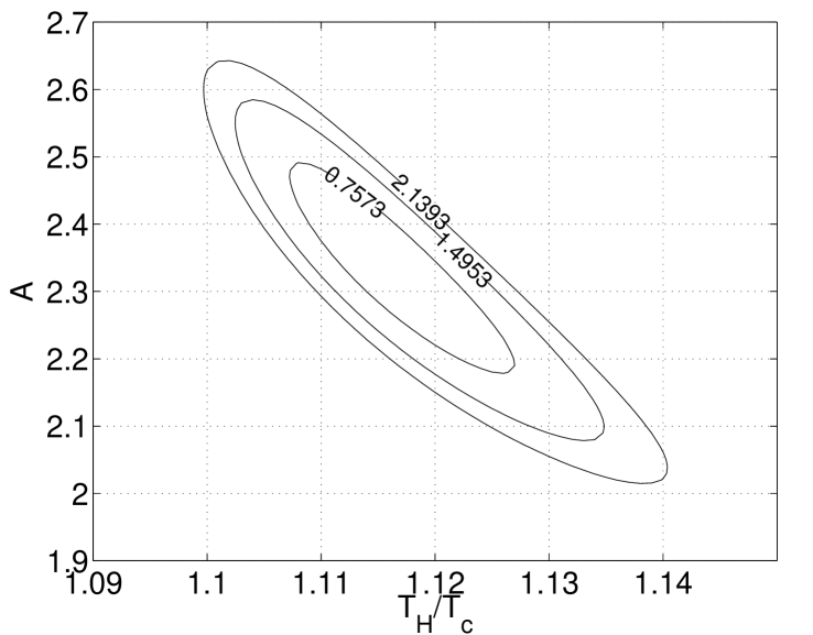
Figure 10: Confidence levels for the fits of $SU(12)$ obtained with method B, with mean-field theory and 3D XY exponents. The plot on the right is for the 3D XY exponent, and on the left with a mean-field theory exponent.

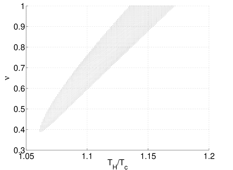
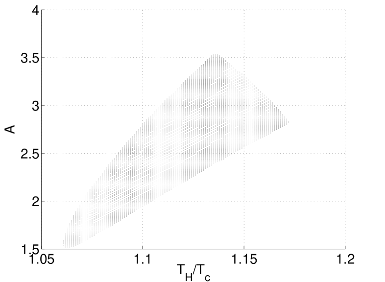
Figure 11: Two dimensional projections of a isosurface in the three-dimensional space of $(\nu,T_{H}/T_{c},A)$ which represents a confidence level of $68.27\%$ for the fits of $SU(12)$ obtained with method B, with a free exponent.

III Summary and discussion

Gathering all the statistically reliable results of $SU(10)$, we find that $T_{H}/T_{c}=1.104(6)-1.114(15)$ when fitting with a 3D XY exponent. When $\nu$ was treated as a free parameter fit we find central values of $\nu=1$ and $T_{H}/T_{c}=1.160-1.172$. Finally when a mean-field exponent is used, one find from data obtained with method B that $T_{H}/T_{c}=1.087(11)$. We also find that the extrapolation with the mean-field exponent has a higher $\chi^{2}$, both in the case of method A, and in the case of method B on a $14^{3}5$ lattice. In particular, when we analyze both data sets together, we find that the best fit has a $\chi^{2}/{\rm dof}=1.93,1.36$ (with ${\text{d}of}=29$) when fitting with a mean-field, and a 3D XY exponent respectively. It is also interesting that the most sizable contribution to the $\chi^{2}$ in this case comes from the data point at $\beta=68.95$ (also line no. 10 in Table 2). Since no reasonable fit will go through this point (see Fig. 2), it is quite conceivable that at this value of $\beta$ we have a strong statistical fluctuation. Ignoring this point gives essentially the same fitting parameters, but makes $\chi^{2}/{\text{d}of}=1.54,1.04$ for the mean-field and 3D XY exponents respectively. This suggests that the 3D XY exponent is preferable (although we still cannot exclude the mean-field exponent possibility completely). This preference is also be seen in Figs. 7, and 9, where we give the projections in the $\nu-T_{H}/T_{c}$ plane, of a volume in the $(\nu,A,T_{H}/T_{c})$ space, that corresponds to a confidence level of $\leq 68.27\%$. There we see that the point $\nu=0.5$ is either outside, or at the edge of this volume.

For $N=12$ the fits are better, and we find that $T_{H}/T_{c}=1.092(6)-1.116(9)$ for mean-field and 3D XY exponents. Both fits have a low $\chi^{2}$, and we again cannot rule out either. Here again the mean-field fit has a higher $\chi^{2}$ than that of the 3D XY fit. In this case, however, in view of the good $\chi^{2}$ values, the preference towards a 3D XY exponent is weaker than for $SU(10)$. Nonetheless it is interesting that when we perform a fit with the exponent $\nu$ as a free parameter we find $T_{H}/T_{c}=1.119$, and $\nu=0.69$ which is closer to the 3D XY exponent $\nu=0.6715(3)$ than to the mean-field value of $\nu=0.5$. Looking at Fig. 11 we find that the preference of our data for $\nu=0.6715$ is indeed weaker here, as both exponents have a similar position in the parameter space, with respect to the shaded area.

The limited statistics prevents us from making statements about the behavior of $T_{H}$ as a function of $N$. This is unfortunate, since it is of interest to know how far is $T_{H}/T_{c}$ from $1$ at $N=\infty$. Nevertheless we obtain fitted values of $T_{H}/\sqrt{\sigma}\simeq 0.62-0.68$, which is lower than $T_{c}/\sqrt{\sigma}\simeq 0.7$ of $SU(2)$ McLerran and Svetitsky (1981) where the phase transition is second order, and therefore may be Hagedorn, $T_{c}=T_{H}$, or provides a lower bound on $T_{H}$. To emphasize this point we plot the $\sigma_{\rm eff}/\sigma$ for $N=10,12$ that we obtained with method B here. For guidance we also calculate the masses from Polyakov loops for $SU(2)$ on a $L^{3}5$ lattice with $L=16,20$, and $24$. The results are presented in Table 7, and also show the expected increase in finite volume corrections as the temperature approaches $T_{c}$. For each value of $T/\sqrt{\sigma}$ we choose to present in Fig. 12 the corresponding value of $\sigma_{\rm eff}/\sigma$ calculated on the largest volume there, together with an extra point for $SU(2)$ at $T=T_{c}$ with $\sigma_{\rm eff}=0$. For the physical scale we again use the interpolation fit in Lucini et al. (2005). We find that for $N=10,12$ the results seem to be close, but not to follow the $SU(2)$ results.

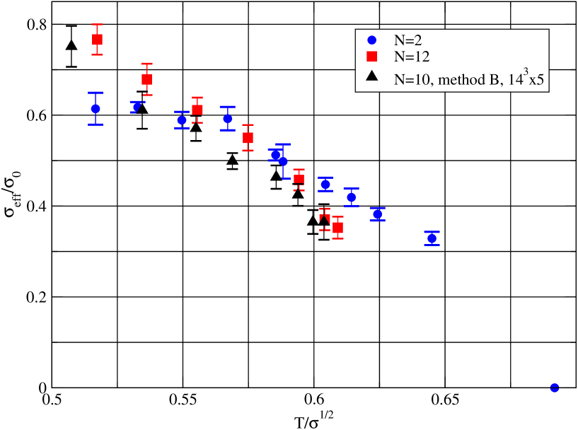
Figure 12: Effective string tension for $N=2,10,12$ in units of the zero temperature string tension.

Table 7: Masses from Polyakov loops on $L^{3}5$ lattices for $N=2$.

loop mass: SU(2)
$\beta$	$16^{3}5$	$20^{3}5$	$24^{3}5$	$a\sqrt{\sigma}$
2.28	0.472(11)	0.476(13)	0.460(26)	0.3871
2.29	0.439(9)	0.435(8)	-	0.3754
2.295	0.417(22)	-	0.383(22)	0.3639
2.30	0.373(11)	0.390(12)	-	0.3527
2.31	0.359(8)	0.335(8)	0.368(16)	0.3417
2.32	0.303(8)	0.299(9)	0.299(7)	0.3400
2.3215	0.290(19)	-	0.288(22)	0.3309
2.33	0.274(8)	0.252(8)	0.245(8)	0.3256
2.335	0.252(11)	-	0.222(10)	0.3204
2.34	0.217(8)	0.205(7)	0.196(7)	0.3101
2.35	0.161(6)	0.158(7)	0.158(7)	0.2891

Finally we find interesting the fact that the Nambu-Goto action, gives rises to a Hagedorn behavior at similar temperatures given by

$$T^{\text{NG}}_{c}/\sqrt{\sigma}\simeq 0.691/\sqrt{c},$$ (9)

where $c$ is the central charge Meyer and Teper (2004) and equals unity in the usual Nambu-Goto model. Applying this formula to our values of $T_{H}$ we give the central charge values listed in Table 6.

A determination of the proper universality class is an important issue, and may teach us how the scaling region behaves with $N$ (if at $T_{H}$ the system behaves like in a second order transition). As mentioned in the introduction, this question was studied numerically in Chandrasekharan and Strouthos (2005) for the strongly-coupled gauge theory (with quarks included), and analytically in Bringoltz (2005) where the scaling region for chiral restoration was seen not to change with $N$. In our context the similar question can be approached for deconfinement in the continuum of the pure gauge theory. Unfortunately, despite the mild preference towards the 3D XY model, discussed above, we currently cannot rule out unambiguously any of the universality classes. To distinguish which one is actually correct one must approach $T_{H}$ closer, and increase the statistics. In fact, as discussed in the introduction, if the Hagedorn transition is second order, we expect that the critical region shrinks with increasing $N$, and that only when $(T_{H}-T)\stackrel{{\scriptstyle<}}{{{}_{\sim}}}1/N^{4}$, one will see the nontrivial critical behavior of a 3DXY model. This is however hard because tunneling configurations become more probable, and finite volume effects (although relatively small at larger values of $N$) become more important. Nonetheless when we perform a fit with the critical exponent $\nu\in[0,1]$ as a free parameter we find that for $SU(12)$, the best fit result for $\nu$ is closer to the 3D XY exponent than to the mean-field value.

We believe that a more thorough investigation (with larger statistics) would render the understanding of the proper universality class, and indeed all the other issues discussed above, much clearer, and the large–$N$ limit of the gauge theory better understood. However, considering its current numerical cost we postpone it to future studies. A different route to approach this question is to study variants of the pure gauge theory, such as adding scalar fields. Depending on the couplings added, the phase transition can become second order Aharony et al. (2005), and one can study the adequacy of large-$N$ mean-field techniques close to second order phase transition in a thermodynamically stable phase.