Clebsch-Gordan Construction of Lattice Interpolating Fields for Excited Baryons

Abstract

Large sets of baryon interpolating field operators are developed for use in lattice QCD studies of baryons with zero momentum. Operators are classified according to the double-valued irreducible representations of the octahedral group. At first, three-quark smeared, local operators are constructed for each isospin and strangeness and they are classified according to their symmetry with respect to exchange of Dirac indices. Nonlocal baryon operators are formulated in a second step as direct products of the spinor structures of smeared, local operators together with gauge-covariant lattice displacements of one or more of the smeared quark fields. Linear combinations of direct products of spinorial and spatial irreducible representations are then formed with appropriate Clebsch-Gordan coefficients of the octahedral group. The construction attempts to maintain maximal overlap with the continuum $SU(2)$ group in order to provide a physically interpretable basis. Nonlocal operators provide direct couplings to states that have nonzero orbital angular momentum.

I Introduction

The theoretical determination of the spectrum of baryon resonances from QCD continues to be an important goal. Lattice QCD calculations have succeeded in part to meet this goal by providing results for the lowest-mass baryon of each isospin in the quenched approximation using overly large masses for the $u$ and $d$ quarks. Aoki03 ; Weingarten93

Most lattice simulations to date have used restricted sets of operators appropriate for $J^{P}=1/2^{\pm},3/2^{\pm}$ states. Masses of low-lying, positive-parity baryons are reproduced with approximately 10% deviations from experimental values using the quenched approximation Aoki03 . Much less is known about higher-spin excited states. The first preliminary lattice calculation of $5/2^{\pm}$ $N^{*}$ masses was reported by the Lattice Hadron Physics Collaboration Basak04 using one of the operators that we develop in this paper Sato04 . Results for excited baryons were also reported based on the use of different radial smearings of the quarks in Refs. BGR04 ; BGR05 . Recently, studies of negative-parity baryons have been reported by several groups Kyoto03 ; Gockeler02 ; Sasaki05 ; Sasaki02 ; Adelaide03 ; Leinweber03 ; Regensburg03 . Nemoto et al. and Melnitchouk et al. considered the $\Lambda(1405)$ baryon, which is the lightest negative-parity baryon despite its nonzero strangeness. They used a three-quark interpolating field operator motivated by the spin-flavor $SU(6)$ quark model and concluded that $\Lambda(1405)$ was not evident in their lattice calculations.

To improve upon our understanding of the resonance spectrum, correlation matrices will be needed, necessitating the construction of sufficiently large sets of baryon and multi-hadron operators. The correlation-matrix method michael85 ; lw90 has been used to determine the spectrum of glueball masses by Morningstar and Peardon Morningstar99 . A large number of interpolating field operators was used to form matrices of lattice correlation functions. The spectrum of effective masses was obtained by diagonalizing the matrices of correlation functions to isolate mass eigenstates for each symmetry channel. In effect, one allows the dynamics to determine the optimal linear combination of operators that couple to each mass state. A similar program for baryons is being undertaken by the Lattice Hadron Physics Collaboration. The first step is to determine a large number of suitable baryon interpolating field operators that correspond to states of zero momentum, definite parity and values of angular momentum $J={1\over 2},{3\over 2},{5\over 2},\cdots$.

Due to the complexity of the operator construction and the importance of providing checks on the final results, we have been pursuing two different approaches. An alternative method, based on a computational implementation of the group projection operation, is presented elsewhere Morningstar04 ; Basak05 .

On a cubic lattice, the continuum rotational symmetry is broken to the finite octahedral group, $O$. States of definite angular momentum correspond to states that occur in certain patterns distributed over the irreducible representations (IRs) of $O$. Although mass calculations are insensitive to the spin projection $J_{z}$, other applications do require baryons with a definite spin projection. We develop operators that are IRs of $O$ using a basis that corresponds as closely as possible to the continuum $J,J_{z}$ states in order to have operators for applications that require spin projection.

It is important to use smearing of the quark fields and to have nonlocal baryon operators as well as the usual local operators. Smeared and nonlocal operators provide a variety of radial and angular distributions of quarks within a baryon so as to couple efficiently to excited states. Nonlocal operators are needed in order to realize spins $J>{3\over 2}$ and simply to enlarge the sets of operators.

In this paper, we first review some basic facts about the octahedral group for integer and half-integer spins in Section II Johnson ; Elliott ; Altmann ; Mandula83 ; Mandula82 ; Butler and review a useful notation for Dirac indices based on $\rho$-spin. Two basic types of three-quark operators are considered: quasi-local and nonlocal. Each quark field in a quasi-local baryon operator is smeared about a common point ${\bf x}$ using the same cubically symmetric form of smearing. Quasi-local operators include local operators as a special case, i.e., when the smearing is omitted. We develop IRs for quasi-local operators in Section III for each baryon: $N$, $\Delta$, $\Lambda$, $\Sigma$, $\Xi$ and $\Omega$. This amounts to determining all allowed combinations of Dirac indices for each flavor symmetry and classifying them into IRs of the octahedral group.

The quasi-local operators provide templates that are used for the construction of nonlocal operators in Section IV. Nonlocal operators are formed by applying extra lattice displacements to one (or more) of the smeared quark fields, thus providing a smearing distribution that differs from that used for the other quarks. In the simplest case, the combination of extra displacements used is cubically symmetric and only changes the radial distribution of the smearing. In other cases the combinations of the extra displacements transform as IRs of the octahedral group, and are chosen to correspond as closely as possible to spherical harmonics. The IRs of lattice displacements and IRs of Dirac indices are combined to form overall IRs for the nonlocal operators using an appropriate set of Clebsch-Gordan coefficients of the octahedral group. Some concluding remarks are presented in Section V.

II Octahedral Group and Lattice Operators

In lattice QCD, hadron field operators are composed of quark and gluon fields on a spatially-isotropic cubic lattice. The lattice is symmetric with respect to a restricted set of rotations about spatial axes that form the octahedral group, $O$, which is a subgroup of the continuum rotational group $SU(2)$. The octahedral group consists of 24 group elements, each corresponding to a discrete rotation that leaves invariant a cube, or an octahedron embedded within the cube. When the objects that are rotated involve half-integer values of the angular momentum, the number of group elements doubles to extend the range of rotational angles from $2\pi$ to $4\pi$, forming the double-valued representations of the octahedral group, referred to as $O^{D}$.

Spatial inversion commutes with all rotations and together with the identity forms a two-element point group. Taking inversion together with the finite rotational group simply doubles the number of group elements, giving the group $O^{D}_{h}$ for half-integer spins.

Given a lattice interpolating operator for a baryon, one may generate other operators by applying the elements of $O^{D}_{h}$ to the given operator. This produces a set of operators that transform amongst themselves with respect to $O^{D}_{h}$, and thus these operators ${\cal O}_{i}$ form the basis of a representation of the group. When a group element $G_{a}$ is applied to operator ${\cal O}_{i}$ in the set, the result is a linear combination of other operators in the set, $\sum_{j}{\cal O}_{j}T_{ji}(G_{a})$, where $T_{ji}(G_{a})$ is a matrix representation of the octahedral group. Such matrix representations are in general reducible. In order to identify operators that correspond to baryons with specific lattice symmetries, it is necessary to block-diagonalize $T_{ji}$, each block corresponding to an irreducible representation of the octahedral group. This task is facilitated by a judicious choice of IR basis vectors for the octahedral group, such as the “cubic harmonics” or “lattice harmonics” of Refs. Cracknell ; Dirl .

II.1 Integer angular momentum : $O$

The octahedral group $O$ has five IRs, namely $A_{1},A_{2},E,T_{1}$ and $T_{2}$ with dimension 1, 1, 2, 3 and 3, respectively, where we follow the conventions of Ref. Johnson . The patterns of IRs of $O$ that correspond to IRs of the continuum rotational group $SU(2)$ with spin $J$ are shown in Table 1.

Table 1: The subduction of $SU(2)$ to IR $\Lambda$ of $O$ for integer $J$.

$J$		$\Lambda$
$0$		$A_{1}$
$1$		$T_{1}$
$2$		$E\oplus T_{2}$
$3$		$A_{2}\oplus T_{1}\oplus T_{2}$
$4$		$A_{1}\oplus E\oplus T_{1}\oplus T_{2}$

A $J=$0 state must show up in the $A_{1}$ IR, but in no other IR of $O$. A $J=$ 1 state must show up in the $T_{1}$ IR but in no other IR. A $J=$ 2 state must show up in the $E$ and $T_{2}$ IRs.

Lattice displacements form representations of $O$ corresponding to integer angular momenta. We choose the standard “lattice harmonics” that are shown in Table 2 as the appropriate basis vectors because they have a straightforward connection to IRs of the rotation group $SU(2)$ in the continuum limit.

Table 2: Basis of irreducible representations of $O$ in terms of spherical harmonics, $Y_{l,m}$ for the lowest values of $l$. $d_{\Lambda}$ is the dimension of the IR. The lattice harmonics are understood to be evaluated on a cubic lattice.

$\Lambda$	$d_{\Lambda}$	row 1	row 2	row 3
$A_{1}$	1	$Y_{0,0}$	$-$	$-$
$A_{2}$	1	${1\over\sqrt{2}}(Y_{3,2}-Y_{3,-2})$	$-$	$-$
$E$	2	$Y_{2,0}$	${1\over\sqrt{2}}(Y_{2,2}+Y_{2,-2})$	$-$
$T_{1}$	3	$Y_{1,1}$	$Y_{1,0}$	$Y_{1,-1}$
$T_{2}$	3	$Y_{2,1}$	${1\over\sqrt{2}}(Y_{2,2}-Y_{2,-2})$	$Y_{2,-1}$

For example, the $Y_{1,m}$ spherical harmonics for $m=1,0,-1$ provide a basis for the three-dimensional $T_{1}$ IR. The same basis convention for $T_{1}$ appears in Ref. Wingate95 , and the same basis convention for $E$ appears in Ref. Lacock96 .

Any quantities that transform in the same fashion as the basis vectors provide a suitable IR for the octahedral group. We will show in Section IV how to use combinations of lattice displacements of quark fields in order to realize the same transformations as the “lattice harmonics”.

II.2 Half-integer angular momenta: $O^{D}$

The eight IRs of the double-valued representations of the octahedral group, $O^{D}$, include $A_{1},A_{2},E,T_{1},T_{2}$ for integer spins and $G_{1},G_{2}$, and $H$ for half-integer spins. The additional IRs $G_{1},G_{2}$ and $H$ have dimensions 2, 2, and 4, respectively; these are the appropriate IRs for baryon operators on a cubic lattice. Table 3 shows the patterns within $O^{D}$ that correspond to some half-integer values of $J$.

Table 3: The subduction of $SU(2)$ to IR $\Lambda$ of $O^{D}$ for half-integer $J$.

$J$		$\Lambda$
$1/2$		$G_{1}$
$3/2$		$H$
$5/2$		$H\oplus G_{2}$
$7/2$		$G_{1}\oplus H\oplus G_{2}$

For example, a $J=$1/2 baryon state should show up in IR $G_{1}$. A spin 3/2 baryon should show up in IR $H$. A spin 5/2 state should show up in IRs $H$ and $G_{2}$ but not in $G_{1}$. A $J=$7/2 state should show up once in IRs $G_{1}$, $H$ and $G_{2}$.

A suitable set of IR basis vectors for half-integer angular momenta is given by the eigenstates $\left|J,m\right>$ of $J^{2}$ and $J_{z}$ that are listed in Table 4.

Table 4: Correspondence of our choice of rows in the $G_{1}$, $G_{2}$ and $H$ IRs to the eigenstates $\left|J,m\right>$ of $J^{2}$ and $J_{z}$.

$\Lambda$	$d_{\Lambda}$	row 1	row 2
$G_{1}$	2	$\left|{1\over 2},{1\over 2}\right>$	$\left|{1\over 2},-{1\over 2}\right>$
$G_{2}$	2	$\sqrt{\frac{1}{6}}\left|{5\over 2},{5\over 2}\right>-\sqrt{\frac{5}{6}}\left|{5\over 2},-{3\over 2}\right>$	$-\sqrt{\frac{5}{6}}\left|{5\over 2},{3\over 2}\right>+\sqrt{\frac{1}{6}}\left|{5\over 2},-{5\over 2}\right>$

$\Lambda$	$d_{\Lambda}$	row 1	row 2	row 3	row 4
$H$	4	$\left|{3\over 2},{3\over 2}\right>$	$\left|{3\over 2},{1\over 2}\right>$	$\left|{3\over 2},-{1\over 2}\right>$	$\left|{3\over 2},-{3\over 2}\right>$

Explicit forms of the $G_{1}$ and $H$ basis states for products of three Dirac spinors are given in Appendix B. Note that the $G_{2}$ basis cannot be built using three Dirac spinors unless orbital angular momentum is added.

II.3 Smearing and smearing parity

The first step in the construction of field operators suitable for baryons is to specify primitive three-quark operators. Consider a generic operator formed from three-quark fields as follows,

$$\epsilon_{abc}\>\overline{q}_{\mu_{1}}^{af_{1}}({\bf x},t)\overline{q}_{\mu_{2}}^{bf_{2}}({\bf x},t)\overline{q}_{\mu_{3}}^{cf_{3}}({\bf x},t),$$ (1)

where $a$, $b$ and $c$ are color indices, $f_{1}$, $f_{2}$ and $f_{3}$ are flavor indices and $\mu_{1}$, $\mu_{2}$ and $\mu_{3}$ are Dirac indices with values $1$ to $4$. The operator is antisymmetrized in color by the $\epsilon_{abc}$ factor when the (implicit) sums over $a$, $b$ and $c$ are performed.

The use of gauge-covariant quark-field smearing, such as Gaussian smearing Alford96 , Jacobi smearing ukqcd93 or so-called Wuppertal smearing Guesken90 , is important for enhancing the coupling to the low-lying states. Gauge-link smearing Albanese87 ; Hasenfratz01 ; Peardon04 further reduces the coupling to the short-wavelength modes of the theory. Schematically, the smearing replaces each unsmeared field by a sum of fields with a distribution function as follows,

$$q_{\mu}({\bf x},t)=\sum_{y}\hat{G}({\bf x},{\bf x}+{\bf y})\tilde{q}_{\mu}({\bf x}+{\bf y},t),$$ (2)

where $\tilde{q}_{\mu}({\bf x},t)$ denotes an unsmeared field at point ${\bf x}$ and the smearing distribution function $\hat{G}$ is gauge covariant. When the smearing distribution is cubically symmetric about point ${\bf x}$ and is the same for each quark field, the baryon operator of Eq. (1) is referred to as quasi-local. Quasi-local operators have the same transformations under the octahedral group as unsmeared operators.

Nonlocal operators differ because the smearing distribution of one or more quark fields is altered by extra lattice displacements. An example is the covariant derivative formed by a linear combination of two displacements of a smeared quark field,

$$D_{i}q_{\mu}({\bf x},t)=U_{i}({\bf x})q_{\mu}({\bf x}+\hat{i},t)-U^{{\dagger}}_{i}({\bf x}-\hat{i})q_{\mu}({\bf x}-\hat{i},t),$$ (3)

where the color indices are suppressed. Equation (3) defines a new smearing distribution that is odd with respect to an inversion about point ${\bf x}$. Thus, smearing can contribute in a nontrivial way to the behavior of the field with respect to inversion. This we call smearing parity.

II.4 Inversion, Parity and $\rho$-parity

The improper point groups $O_{h}$ and $O^{D}_{h}$ consist of rotations that leave the cube invariant together with the spatial inversion. The parity transformation of a Dirac field involves multiplication by the $\gamma_{4}$ Dirac matrix in addition to spatial inversion as follows,

$${\cal P}\tilde{q}({\bf x},t){\cal P}^{-1}=\gamma_{4}\tilde{q}(-{\bf x},t),$$ (4)

where ${\cal P}$ is the parity operator. Throughout this work we employ the Dirac-Pauli representation for Dirac $\gamma$ matrices for which $\gamma_{4}={\rm diag}[1,1,-1,-1]$. However, our results may be used with any representation of the Dirac $\gamma$ matrices by applying the appropriate unitary transformation as discussed in Appendix A.

It is convenient to express the Dirac matrices as a direct product of the form $SU(2)_{\rho}\otimes SU(2)_{s}$ where the $SU(2)$ components are generated by the 2$\times$2 Pauli matrices for spin s and $\rho$-spin $\rho$ Gammel71 ; Kubis72 . See Appendix A for details of the construction.

Expressed in terms of the $SU(2)_{\rho}\otimes SU(2)_{s}$ matrices, $\gamma_{4}=\rho_{3}\otimes\sigma_{4}$ where $\rho_{3}=\rm{diag}[1,-1]$ and $\sigma_{4}=\rm{diag}[1,1]$. Similarly, the Dirac matrix $\sigma_{21}={i\over 2}[\gamma_{2},\gamma_{1}]=\rho_{4}\otimes\sigma_{3}$ where $\rho_{4}=\rm{diag}[1,1]$ and $\sigma_{3}=\rm{diag}[1,-1]$. With these conventions, a fermion field satisfies

$$\gamma_{4}\tilde{q}_{\mu}({\bf x},t)=(\rho_{3}\otimes\sigma_{4})\tilde{q}_{\mu}({\bf x},t)=\rho\tilde{q}_{\mu}({\bf x},t),$$ (5)

and

$$\sigma_{21}\tilde{q}_{\mu}({\bf x},t)=(\rho_{4}\otimes\sigma_{3})\tilde{q}_{\mu}({\bf x},t)=s\tilde{q}_{\mu}({\bf x},t),$$ (6)

where Table 5 provides the $\rho$ and $s$ values. Thus, the Dirac index $\mu=1,2,3,4$ is equivalent to a two-dimensional superscript corresponding to $\rho$-spin ($\rho$ = +1, -1) and a two-dimensional subscript corresponding to spin ($s=+1,-1$), and the field may be written as $q^{\rho}_{s}({\bf x},t)$. We refer to the $\rho$ value as $\rho$-parity because of its role in the parity transformation of Eqs. (4) and (5).

Table 5: Translation of the Dirac index $\mu$ to $\rho$- and $s$-spin indices. Index $\mu$ is expressed in the Dirac-Pauli representation.

Dirac index $\mu$	$\rho$	$s$
1	$+$	$+$
2	$+$	$-$
3	$-$	$+$
4	$-$	$-$

The parity transformation of a smeared quark field can differ from that of an unsmeared field because the smearing parity enters. This is most easily seen by using free fields for which the gauge link variables are unity. Then the smearing distribution does not depend on the point ${\bf x}$ and reduces to the set of coefficients $c({\bf y})$ that weight the fields at points ${\bf y}$ away from the central point ${\bf x}$, i.e., the smeared quark field is

$$q_{\mu}({\bf x},t)=\sum_{\bf y}c({\bf y})\tilde{q}_{\mu}({\bf x}+{\bf y},t)$$ (7)

and the smearing parity is defined by

$$c(-{\bf y})=pc({\bf y}),$$ (8)

where $p=+1$ or $-1$ for even or odd smearing parity, respectively. The parity transformation of a smeared field is

$${\cal P}q_{\mu}({\bf x},t){\cal P}^{-1} = \sum_{y}c({\bf y})\gamma_{4}\tilde{q}_{\mu}(-{\bf x}-{\bf y},t)$$ (9)

$$= \gamma_{4}\sum_{\bf y}c(-{\bf y})\tilde{q}_{\mu}(-{\bf x}+{\bf y},t),$$

$$= \gamma_{4}p\sum_{y}c({\bf y})\tilde{q}_{\mu}(-{\bf x}+{\bf y},t),$$

$$= \gamma_{4}pq_{\mu}(-{\bf x},t),$$

where the second line involves the relabeling ${\bf y}\rightarrow-{\bf y}$ and the third line uses the symmetry of the smearing distribution under inversion of ${\bf y}$. When the gauge links are included so as to obtain a gauge covariant smearing a similar result is obtained, which holds as an average over gauge configurations.

The parity transformation of a product of three smeared quark fields is

$${\cal P}q^{\rho_{1}}_{s_{1}}({\bf x},t)q^{\rho_{2}}_{s_{2}}({\bf x},t)q^{\rho_{3}}_{s_{3}}({\bf x},t){\cal P}^{-1}=$$

$$\rho_{1}\rho_{2}\rho_{3}\,\,p_{1}p_{2}p_{3}\,\,q^{\rho_{1}}_{s_{1}}(-{\bf x},t)q^{\rho_{2}}_{s_{2}}(-{\bf x},t)q^{\rho_{3}}_{s_{3}}(-{\bf x},t),$$ (10)

where we have used the notation $q_{s}^{\rho}({\bf x},t)$ in place of $q_{\mu}({\bf x},t)$ and evaluated the $\gamma_{4}$ matrices using Eq. (5) to obtain the product of the three $\rho$-parities. The product $\rho_{1}\rho_{2}\rho_{3}$ is referred to simply as the $\rho$-parity of the operator and the product $p_{1}p_{2}p_{3}$ is referred to as the smearing parity of the operator.

The field operator at an arbitrary point ${\bf x}$ does not have a definite parity. However, in correlation functions projected to zero total momentum, the ${\bf x}$ dependence is removed by a translation following insertion of a complete set of intermediate states, e.g.,

$$C(t) = \sum_{\bf x}<0|B({\bf x},t)\bar{B}({\bf 0},0)|0>$$

$$= \sum_{n}<0|B({\bf 0},0)|n>e^{-M_{n}t}<n|\bar{B}({\bf 0},0)|0>.$$

Thus the zero-momentum correlation function has baryon operators only at point ${\bf x}={\bf 0}$ where the operator has parity given by the product of $\rho$-parity and smearing parity, i.e., $\rho_{1}\rho_{2}\rho_{3}\,\,p_{1}p_{2}p_{3}$ in Eq. (10). The parity of intermediate state $n$ must be the same in order to have a nonvanishing coupling.

Rotations of a quark field are generated by the Dirac matrices $\sigma_{ij}=-\rho_{4}\otimes\sigma_{k}$ where indices i, j and k are cyclic and take the values 1, 2 and 3. Rotations are diagonal in $\rho$-spin and thus give a linear combination of fields with different $s$ labels but the same $\rho$-parity,

$$U(R)\overline{q}_{s}^{\rho}({\bf x},t)U^{{\dagger}}(R)=\sum_{s^{\prime}}\overline{q}_{s^{\prime}}^{\rho}(R^{-1}{\bf x},t)T_{s^{\prime}s}(R),$$ (12)

where $T_{s^{\prime}s}(R)$ is a representation matrix of rotation $R$. This insight into the transformations of Dirac indices with respect to rotations is the first reason that we find the $\rho,s$ labels useful.

Note that a “barred” field transforms in the same way as a quantum “ket” when the unitary quantum operator $U(R)$ is applied, i.e.,

$$U(R)\left|s\right>=\sum_{s^{\prime}}\left|s^{\prime}\right>\left<s^{\prime}\right|U(R)\left|s\right>=\sum_{s^{\prime}}\left|s^{\prime}\right>T_{s^{\prime}s}(R).$$ (13)

However,“unbarred” fields also are required. Although they are independent fields in the Euclidean theory, their transformations are similar to those of quantum “bra” states,

$$U(R)q_{s}^{\rho}({\bf x},t)U^{{\dagger}}(R)=\sum_{s^{\prime}}q_{s^{\prime}}^{\rho}(R^{-1}{\bf x},t)T^{{\dagger}}_{ss^{\prime}}(R).$$ (14)

In this paper we state results generally in terms of “barred” fields in order to have a transparent connection between the transformations of fields and those of the quantum states that they create. “Unbarred” operators generally involve the same constructions except that coefficients or other operators involved must be hermitian conjugated.

Operators that couple only to even parity intermediate states in Eq. (LABEL:eq:correlfn) are labeled with a subscript $g$ (for gerade) and operators that couple only to odd parity states are labeled with a subscript $u$ (for ungerade). For half-integer spins, the relevant IRs of $O^{D}_{h}$ are: $G_{1g},G_{2g},H_{g},G_{1u},G_{2u},H_{u}$. We will use these notations throughout this paper.

Because of the parity transformation of Eq. (10), there are two independent ways to make baryon operators that couple to states of a given parity in a zero-momentum correlation function. Operators coupling to gerade states can be made either with even smearing parity together with positive $\rho$-parity or with odd smearing parity together with negative $\rho$-parity. Similarly, there are two disjoint sets of operators that couple to ungerade states: ones with odd smearing parity together with positive $\rho$-parity or ones with even smearing parity together with negative $\rho$-parity. These sets are not connected by rotations because neither the smearing parity nor the $\rho$-parity can be changed by a rotation. However, they are connected by $\rho$-spin raising or lowering operations and in our construction each operator that couples to a gerade state is connected in this way with an operator that couples to an ungerade state. This is the second reason that the $\rho,s$ labeling is useful. The $\rho,s$ labeling is used sparingly in this paper but it is central to the method used in Appendix B to construct combinations of Dirac indices that transform irreducibly.

Each baryon operator carries a row label, $\lambda$, whose meaning depends upon the bases used for IRs. The row label distinguishes between the $d_{\Lambda}$ members of IR $\Lambda$. If a representation contains more than one occurrence of IR $\Lambda$, we say that there are multiple embeddings of that IR. A superscript, $k$, is used to distinguish between the different embeddings. Therefore, a generic baryon operator is denoted as $\overline{B}^{\Lambda,k}_{\lambda}({\bf x},t)$, or in “unbarred” form as $B^{\Lambda,k}_{\lambda}({\bf x},t)$, where the operator belongs to the $k^{th}$ embedding of IR $\Lambda$ and row $\lambda$ of the octahedral group. Operators for different baryons are indicated by the use of appropriate symbols, such as $\overline{N}^{\Lambda,k}_{\lambda}({\bf x},t)$ (for isospin 1/2 operators), $\overline{\Delta}^{\Lambda,k}_{\lambda}({\bf x},t)$ (for isospin 3/2 operators), $\overline{\Sigma}^{\Lambda,k}_{\lambda}({\bf x},t)$, and so on.

The correlations of operators belonging to different IRs or to different rows of the same IR vanish:

$$\sum_{x}\left<0\right|TB^{\Lambda,k}_{\lambda}({\bf x},t)\overline{B}^{\Lambda^{\prime},k^{\prime}}_{\lambda^{\prime}}(0)\left|0\right>=C^{(\Lambda)}_{kk^{\prime}}(t)\delta_{\Lambda\Lambda^{\prime}}\delta_{\lambda\lambda^{\prime}}.$$ (15)

The correlations of different embeddings of the same IR and row are generally nonzero, providing sets of operators suitable for constructing a correlation matrix $C^{(\Lambda)}_{kk^{\prime}}(t)$.

III Quasi-local Baryonic Operators

Since the quark fields are Grassmann-valued and taken at a common location ${\bf x}$, and the color indices are contracted with the antisymmetric Levi-Civita tensor, our three-quark, quasi-local baryon operators must be symmetric with respect to simultaneous exchange of flavor and Dirac indices. An operator that is symmetric in flavor labels ($\overline{\Delta},\overline{\Omega}$) must be symmetric also in Dirac indices, and an operator that is mixed-antisymmetric in flavor labels ($\overline{N}$) must be mixed antisymmetric in Dirac indices, assuming that masses of the up and down quarks are equal. An operator that is mixed-antisymmetric in flavor labels and that has nonzero strangeness ($\overline{\Lambda}$) can have mixed-antisymmetric or totally antisymmetric Dirac indices, and an operator that is mixed-symmetric in flavor labels and that has nonzero strangeness ($\overline{\Sigma},\overline{\Xi}$) can have mixed-symmetric or totally symmetric Dirac indices. All possible symmetries of the Dirac indices are encountered in the consideration of the different baryons. In this section, we discuss the different baryons in turn and develop tables of operators classified according to IRs of $O_{h}^{D}$.

III.1 Quasi-local Nucleon Operators

Consider operators made from quasi-local quark fields for isospin quantum numbers $I=1/2,I_{z}=1/2$. These operators correspond to the $N^{*}$ family of baryons and they may be chosen to be

$$\overline{N}^{+\rm(MA)}_{\mu_{1}\mu_{2}\mu_{3}}=\epsilon_{abc}{1\over\sqrt{2}}\left(\bar{u}_{\mu_{1}}^{a}\bar{d}_{\mu_{2}}^{b}-\bar{d}_{\mu_{1}}^{a}\bar{u}_{\mu_{2}}^{b}\right)\bar{u}_{\mu_{3}}^{c},$$ (16)

where $u$ is an up quark and $d$ is a down quark. All (smeared) quark fields are defined at spacetime point $({\bf x},t)$. Equation (16) provides a proton operator in the notation of the Particle Data Group PDG . A neutron or $\overline{N}^{0}$ operator can be obtained using the isospin lowering operation.

	$\bigoplus$		$\bigoplus$
MA		MS		S

Figure 1: Young tableaux for three-quark $SU(2)_{I}$ irreducible representations. The first tableau is antisymmetric in labels of particles 1 and 2 (denoted MA for mixed-antisymmetric), while the second tableau is symmetric in the labels of particles 1 and 2 (denoted MS for mixed-symmetric). The third tableau is fully symmetric (denoted S).

These two operators correspond to the mixed-antisymmetric Young tableau for isospin in Fig. 1. Each $N^{\rm(MA)}_{\mu_{1}\mu_{2}\mu_{3}}({\bf x},t)$ operator of Eq. (16) is manifestly antisymmetric with respect to the flavor interchange $u\leftrightarrow d$ applied to the first two quark fields. This leads to the following restrictions on Dirac indices,

$$\overline{N}^{\rm(MA)}_{\mu_{1}\mu_{2}\mu_{3}}+\overline{N}^{\rm(MA)}_{\mu_{2}\mu_{1}\mu_{3}} = 0,$$ (17)

$$\overline{N}^{\rm(MA)}_{\mu_{1}\mu_{2}\mu_{3}}+\overline{N}^{\rm(MA)}_{\mu_{2}\mu_{3}\mu_{1}}+\overline{N}^{\rm(MA)}_{\mu_{3}\mu_{1}\mu_{2}} = 0.$$ (18)

Some general considerations are stated most simply using the Dirac indices. There are 4${}^{3}=$64 combinations of Dirac indices for operators formed from three quark fields. They may be classified by the four Young tableaux of Fig. 2, where each box is understood to take the values $\mu=1,2,3$ or $4$.

	$\bigoplus$		$\bigoplus$		$\bigoplus$
S		MS		MA		A
20		20		20		4

Figure 2: Young tableaux for three Dirac indices.

Standard rules for counting the dimensions of the tableaux show that the totally symmetric tableau includes 20 operators, the mixed-symmetric and mixed-antisymmetric tableaux each have 20 operators and the totally antisymmetric tableau has 4 operators, thus accounting for all 64 possibilities. Groupings of Dirac indices according to the symmetries of Fig. 2 are useful. The fact that a quasi-local baryonic operator must be symmetric with respect to simultaneous exchange of flavor labels and Dirac indices associates each baryon operator with one of the symmetries of Dirac indices found in the tableaux of Fig. 2. All the combinations of Dirac indices that correspond to each Young tableau are given explicitly in Appendix B. Three Dirac spinors whose spin indices are written in accord with one Young tableau in Fig. 2 form a closed set under the group of rotations and parity transformations. These group representations have been reduced to $G_{1g/u}$ and $H_{g/u}$ IRs of Dirac indices by working with the $\rho,s$ labeling as discussed in Appendix B.

Nucleon operators with MA isospin symmetry in Eq. (16) must have the MA symmetry of Dirac indices, corresponding to the third tableau of Fig. 2. Table 6 gives explicit forms for the 20 quasi-local nucleon operators classified into IRs $G_{1g},H_{g},G_{1u},$ and $H_{u}$. Here and in the remainder of this paper we label the operators by the parity of intermediate states to which they couple in a zero-momentum correlation function, as in Eq. (LABEL:eq:correlfn). Alternatively, one may regard the operators in the tables as having been translated to point ${\bf x}={\bf 0}$, where they have definite parity as seen from Eq. (9). Dirac indices in the table come from Table 16 in Appendix B, but they have been simplified using the relation in Eq. (17).

Table 6: Quasi-local Nucleon operators. All operators have MA Dirac indices.

$\overline{\Psi}^{\Lambda,k}_{S,S_{z}}$	$\overline{N}_{\mu_{1}\mu_{2}\mu_{3}}$	$\overline{\Psi}^{\Lambda,k}_{S,S_{z}}$	$\overline{N}_{\mu_{1}\mu_{2}\mu_{3}}$
$\overline{\Psi}^{G_{1g},1}_{{1\over 2},{1\over 2}}$	$\overline{N}_{121}$	$\overline{\Psi}^{G_{1u},1}_{{1\over 2},{1\over 2}}$	${1\over\sqrt{3}}(\overline{N}_{123}\!\!+\!\!\overline{N}_{141}\!\!+\!\!\overline{N}_{321})$
$\overline{\Psi}^{G_{1g},1}_{{1\over 2},-{1\over 2}}$	$\overline{N}_{122}$	$\overline{\Psi}^{G_{1u},1}_{{1\over 2},-{1\over 2}}$	${1\over\sqrt{3}}(\overline{N}_{124}\!\!+\!\!\overline{N}_{142}\!\!+\!\!\overline{N}_{322})$
$\overline{\Psi}^{G_{1g},2}_{{1\over 2},{1\over 2}}$	${1\over\sqrt{3}}(\overline{N}_{143}\!\!+\!\!\overline{N}_{323}\!\!+\!\!\overline{N}_{341})$	$\overline{\Psi}^{G_{1u},2}_{{1\over 2},{1\over 2}}$	$\overline{N}_{343}$
$\overline{\Psi}^{G_{1g},2}_{{1\over 2},-{1\over 2}}$	${1\over\sqrt{3}}(\overline{N}_{144}\!\!+\!\!\overline{N}_{324}\!\!+\!\!\overline{N}_{342})$	$\overline{\Psi}^{G_{1u},2}_{{1\over 2},-{1\over 2}}$	$\overline{N}_{344}$
$\overline{\Psi}^{G_{1g},3}_{{1\over 2},{1\over 2}}$	${1\over\sqrt{3}}(\overline{N}_{134}\!\!+\!\!\overline{N}_{323}\!\!-\!\!\overline{N}_{341})$	$\overline{\Psi}^{G_{1u},3}_{{1\over 2},{1\over 2}}$	${1\over\sqrt{3}}(\!-\!\overline{N}_{141}\!\!-\!\!\overline{N}_{312}\!\!+\!\!\overline{N}_{123})$
$\overline{\Psi}^{G_{1g},3}_{{1\over 2},-{1\over 2}}$	${1\over\sqrt{3}}(\overline{N}_{144}\!\!+\!\!\overline{N}_{423}\!\!-\!\!\overline{N}_{342})$	$\overline{\Psi}^{G_{1u},3}_{{1\over 2},-{1\over 2}}$	${1\over\sqrt{3}}(\!-\!\overline{N}_{322}\!\!-\!\!\overline{N}_{241}\!\!+\!\!\overline{N}_{124})$
$\overline{\Psi}^{H_{g}}_{{3\over 2},{3\over 2}}$	$\overline{N}_{133}$	$\overline{\Psi}^{H_{u}}_{{3\over 2},{3\over 2}}$	$\overline{N}_{131}$
$\overline{\Psi}^{H_{g}}_{{3\over 2},{1\over 2}}$	${1\over\sqrt{3}}(\overline{N}_{134}\!\!+\!\!\overline{N}_{143}\!\!+\!\!\overline{N}_{233})$	$\overline{\Psi}^{H_{u}}_{{3\over 2},{1\over 2}}$	${1\over\sqrt{3}}(\overline{N}_{132}\!\!+\!\!\overline{N}_{141}\!\!+\!\!\overline{N}_{231})$
$\overline{\Psi}^{H_{g}}_{{3\over 2},-{1\over 2}}$	${1\over\sqrt{3}}(\overline{N}_{144}\!\!+\!\!\overline{N}_{234}\!\!+\!\!\overline{N}_{243})$	$\overline{\Psi}^{H_{u}}_{{3\over 2},-{1\over 2}}$	${1\over\sqrt{3}}(\overline{N}_{142}\!\!+\!\!\overline{N}_{232}\!\!+\!\!\overline{N}_{241})$
$\overline{\Psi}^{H_{g}}_{{3\over 2},-{3\over 2}}$	$\overline{N}_{244}$	$\overline{\Psi}^{H_{u}}_{{3\over 2},-{3\over 2}}$	$\overline{N}_{242}$

Because all the coefficients are real, “unbarred” operators are obtained by replacing $\overline{N}$ by $N$ in the same linear combinations . The left column of the table shows 10 gerade nucleon operators and the right one shows 10 ungerade operators. For a given parity there are three sets of $G_{1}$ operators (three embeddings of $G_{1}$) and one set of $H$ operators. Each $G_{1}$ IR contains two operators that transform amongst themselves under rotations of the group and each $H$ IR contains four operators that transform amongst themselves. Operators in each IR are given spin projection labels, $S_{z}$, which are also equivalent to “row” labels but more physically meaningful. In a given embedding the operator with the largest $S_{z}$ is designated “row 1”, the next largest $S_{z}$ is designated “row 2”, and so on. The notation $\overline{\Psi}^{\Lambda,k}_{S,S_{z}}$ represents a general quasi-local baryonic operator with spin $S$ and spin projection $S_{z}$, transforming according to the $k$-th embedding of IR $\Lambda$ of the group $O^{D}_{h}$.

Spin-raising and spin-lowering operators for a Dirac spinor are

$$s^{\pm}={1\over 2}\left(\begin{array}[]{cc}\sigma_{1}\pm i\sigma_{2}&0\\ 0&\sigma_{1}\pm i\sigma_{2}\end{array}\right),$$ (19)

in the Dirac-Pauli representation. For a three-quark state, the spin raising or lowering operator is a sum of three terms, for example, $S^{-}=\sum_{j=1}^{3}s_{j}^{\pm}$, where $s^{\pm}_{j}$ acts on the $j$-th quark. The same operations carry over to the “barred” field operators of Table 6. Different rows in the same embedding of an IR are related to one another by spin raising and lowering operations. For example, the transformation of the first $G_{1}$ embedding of Table 6 proceeds schematically as follows,

$$S^{-}\overline{\Psi}^{G_{1g},1}_{1/2,1/2}=S^{-}\overline{N}_{121} = S^{-}\overline{N}^{+++}_{+-+}$$ (20)

$$= \overline{N}^{+++}_{+--}=\overline{N}_{122}=\overline{\Psi}^{G_{1g},1}_{1/2,-1/2},~{}$$

where the notation $\overline{N}^{\rho_{1}\rho_{2}\rho_{3}}_{s_{1}s_{2}s_{3}}$ is used in the intermediate steps. Note that a spin-lowering operation on the second quark in Eq. (20) vanishes because it has spin down and spin-lowering of the first quark also vanishes because $s_{1}^{-}\overline{N}^{+++}_{+-+}=\overline{N}^{+++}_{--+}=0$ by Eq. (17). Spin raising and lowering operations can be applied repeatedly and the following relation holds,

$$0\longleftarrow{\lower 3.1298pt\hbox{${}_{S^{+}}$}}\hskip 8.53581pt\overline{\Psi}^{G_{1g/u},k}_{1/2,1/2}\hskip 5.69054pt{\lower 1.99168pt\hbox{$\longleftarrow$}}{\raise 1.99168pt\hbox{$\longrightarrow$}}{\lower 5.12149pt\hbox{${}_{S^{+}}$}}{\raise 2.84526pt\hbox{${}^{S^{-}}$}}\hskip 8.53581pt\overline{\Psi}^{G_{1g/u},k}_{1/2,-1/2}\longrightarrow{\raise 1.42262pt\hbox{${}^{S^{-}}$}}\hskip 8.53581pt0,$$

$$0\longleftarrow{\lower 3.1298pt\hbox{${}_{S^{+}}$}}\hskip 8.53581pt\overline{\Psi}^{H_{g/u},k}_{3/2,3/2}\hskip 5.69054pt{\lower 1.99168pt\hbox{$\longleftarrow$}}{\raise 1.99168pt\hbox{$\longrightarrow$}}{\lower 5.12149pt\hbox{${}_{S^{+}}$}}{\raise 2.84526pt\hbox{${}^{S^{-}}$}}\hskip 8.53581pt\overline{\Psi}^{H_{g/u},k}_{3/2,1/2}\hskip 5.69054pt{\lower 1.99168pt\hbox{$\longleftarrow$}}{\raise 1.99168pt\hbox{$\longrightarrow$}}{\lower 5.12149pt\hbox{${}_{S^{+}}$}}{\raise 2.84526pt\hbox{${}^{S^{-}}$}}\hskip 8.53581pt\overline{\Psi}^{H_{g/u},k}_{3/2,-1/2}$$

$$\hskip 5.69054pt{\lower 1.99168pt\hbox{$\longleftarrow$}}{\raise 1.99168pt\hbox{$\longrightarrow$}}{\lower 5.12149pt\hbox{${}_{S^{+}}$}}{\raise 2.84526pt\hbox{${}^{S^{-}}$}}\hskip 8.53581pt\overline{\Psi}^{H_{g/u},k}_{3/2,-3/2}\longrightarrow{\raise 1.42262pt\hbox{${}^{S^{-}}$}}\hskip 8.53581pt0.$$ (21)

A gerade operator in a row of Table 6 and the ungerade one in the same row are related to each other by $\rho$-spin raising and lowering operations. For Dirac spinors, the operators are $\rho^{\pm}=\sum_{j=1}^{3}\rho_{j}^{\pm}$, $\rho^{\pm}_{j}=(1/2)(\rho^{1}_{j}\pm i\rho^{2}_{j})$, where $j$ specifies the first, second, or the third quark. An example is

$$\rho^{-}\overline{\Psi}^{G_{1g},1}_{1/2,1/2} = \rho^{-}\overline{N}_{121}=\rho^{-}\overline{N}^{+++}_{+-+},$$ (22)

$$\rightarrow {1\over\sqrt{3}}\left(\overline{N}^{++-}_{+-+}+\overline{N}^{+-+}_{+-+}+\overline{N}^{-++}_{+-+}\right)$$

$$= {1\over\sqrt{3}}\left(\overline{N}_{123}+\overline{N}_{141}+\overline{N}_{321}\right)$$

$$= \overline{\Psi}^{G_{1u},1}_{1/2,1/2},$$

where an appropriate normalization is included in the resultant operator. Note that $\rho$-spin raising and lowering operations change the $\rho$-parity of one quark and thus change the product $\rho_{1}\rho_{2}\rho_{3}$ which is the $\rho$-parity of the operator. However, they preserve the $s$ labels and leave the transformation properties under rotations unchanged.

Mixed-symmetric isospin operators with $I=1/2,I_{z}=1/2$ may also be defined by

$$\overline{N}^{+\rm(MS)}_{\mu_{1}\mu_{2}\mu_{3}}=\epsilon_{abc}\frac{1}{\sqrt{6}}(2\bar{u}_{\mu_{1}}^{a}\bar{u}_{\mu_{2}}^{b}\bar{d}_{\mu_{3}}^{c}-\bar{u}_{\mu_{1}}^{a}\bar{d}_{\mu_{2}}^{b}\bar{u}_{\mu_{3}}^{c}-\bar{d}_{\mu_{1}}^{a}\bar{u}_{\mu_{2}}^{b}\bar{u}_{\mu_{3}}^{c}).$$ (23)

However, for quasi-local operators they can be rewritten in terms of the MA isospin operators defined in Eq. (16) as follows,

$$\overline{N}^{\rm(MS)}_{\mu_{1}\mu_{2}\mu_{3}}=\overline{N}^{\rm(MA)}_{\mu_{3}\mu_{2}\mu_{1}}+\overline{N}^{\rm(MA)}_{\mu_{1}\mu_{3}\mu_{2}},$$ (24)

showing that the quasi-local, MS isospin operators are not linearly independent of quasi-local MA operators. It is sufficient to consider only the MA operators of Eq. (16) in order to construct a complete, linearly independent set of isospin 1/2, quasi-local operators.

Relations of the operators presented in Table 6 to operators that are commonly used in the literature for a nucleon are given in Appendix C.

III.2 Quasi-local $\Delta$ and $\Omega$ Operators

The isospin of a $\Delta$ baryon is 3/2 and there are four different operators corresponding to isospin projections $I_{z}=3/2,1/2,-1/2$, and $-3/2$:

$$\overline{\Delta}^{\,++}_{\mu_{1}\mu_{2}\mu_{3}} = \epsilon_{abc}\>\bar{u}^{a}_{\mu_{1}}\bar{u}^{b}_{\mu_{2}}\bar{u}^{c}_{\mu_{3}},$$

$$\overline{\Delta}^{\,+}_{\mu_{1}\mu_{2}\mu_{3}} = \frac{\epsilon_{abc}}{\sqrt{3}}\left(\bar{u}^{a}_{\mu_{1}}\bar{u}^{b}_{\mu_{2}}\bar{d}^{c}_{\mu_{3}}+\bar{u}^{a}_{\mu_{1}}\bar{d}^{b}_{\mu_{2}}\bar{u}^{c}_{\mu_{3}}+\bar{d}^{a}_{\mu_{1}}\bar{u}^{b}_{\mu_{2}}\bar{u}^{c}_{\mu_{3}}\right),$$

$$\overline{\Delta}^{\,0}_{\mu_{1}\mu_{2}\mu_{3}} = \frac{\epsilon_{abc}}{\sqrt{3}}\left(\bar{u}^{a}_{\mu_{1}}\bar{d}^{b}_{\mu_{2}}\bar{d}^{c}_{\mu_{3}}+\bar{d}^{a}_{\mu_{1}}\bar{u}^{b}_{\mu_{2}}\bar{d}^{c}_{\mu_{3}}+\bar{d}^{a}_{\mu_{1}}\bar{d}^{b}_{\mu_{2}}\bar{u}^{c}_{\mu_{3}}\right),$$

$$\overline{\Delta}^{\,-}_{\mu_{1}\mu_{2}\mu_{3}} = \epsilon_{abc}\>\bar{d}^{a}_{\mu_{1}}\bar{d}^{b}_{\mu_{2}}\bar{d}^{c}_{\mu_{3}},$$

where all fields are defined at spacetime point $({\bf x},t)$. Because of the totally symmetric flavors, the $\Delta$ baryon operators must have totally symmetric combinations of Dirac indices. According to Table 15 in Appendix B there are 20 combinations of totally symmetric Dirac indices. In a color-singlet three-quark operator, the quark fields may be commuted with one another with no change of sign. This allows Dirac indices to be rearranged to a standard order in which they do not decrease from left to right, producing the 20 irreducible operators that are given in Table 7.

Table 7: Quasi-local $\Delta$ operators. All operators have Dirac indices in S.

$\overline{\Psi}^{\Lambda,k}_{S,S_{z}}$	$\overline{\Delta}_{\mu_{1}\mu_{2}\mu_{3}}$	$\overline{\Psi}^{\Lambda,k}_{S,S_{z}}$	$\overline{\Delta}_{\mu_{1}\mu_{2}\mu_{3}}$
$\overline{\Psi}^{G_{1g},1}_{{1\over 2},{1\over 2}}$	$\overline{\Delta}_{134}-\overline{\Delta}_{233}$	$\overline{\Psi}^{G_{1u},1}_{{1\over 2},{1\over 2}}$	$\overline{\Delta}_{114}-\overline{\Delta}_{123}$
$\overline{\Psi}^{G_{1g},1}_{{1\over 2},-{1\over 2}}$	$\overline{\Delta}_{144}-\overline{\Delta}_{234}$	$\overline{\Psi}^{G_{1u},1}_{{1\over 2},-{1\over 2}}$	$\overline{\Delta}_{124}-\overline{\Delta}_{223}$
$\overline{\Psi}^{H_{g},1}_{{3\over 2},{3\over 2}}$	$\overline{\Delta}_{111}$	$\overline{\Psi}^{H_{u},1}_{{3\over 2},{3\over 2}}$	$\sqrt{3}~{}\overline{\Delta}_{113}$
$\overline{\Psi}^{H_{g},1}_{{3\over 2},{1\over 2}}$	$\sqrt{3}~{}\overline{\Delta}_{112}$	$\overline{\Psi}^{H_{u},1}_{{3\over 2},{1\over 2}}$	$\overline{\Delta}_{114}+2\overline{\Delta}_{123}$
$\overline{\Psi}^{H_{g},1}_{{3\over 2},-{1\over 2}}$	$\sqrt{3}~{}\overline{\Delta}_{122}$	$\overline{\Psi}^{H_{u},1}_{{3\over 2},-{1\over 2}}$	$2\overline{\Delta}_{124}+\overline{\Delta}_{223}$
$\overline{\Psi}^{H_{g},1}_{{3\over 2},-{3\over 2}}$	$\overline{\Delta}_{222}$	$\overline{\Psi}^{H_{u},1}_{{3\over 2},-{3\over 2}}$	$\sqrt{3}~{}\overline{\Delta}_{224}$
$\overline{\Psi}^{H_{g},2}_{{3\over 2},{3\over 2}}$	$\sqrt{3}~{}\overline{\Delta}_{133}$	$\overline{\Psi}^{H_{u},2}_{{3\over 2},{3\over 2}}$	$\overline{\Delta}_{333}$
$\overline{\Psi}^{H_{g},2}_{{3\over 2},{1\over 2}}$	$2\overline{\Delta}_{134}+\overline{\Delta}_{233}$	$\overline{\Psi}^{H_{u},2}_{{3\over 2},{1\over 2}}$	$\sqrt{3}~{}\overline{\Delta}_{334}$
$\overline{\Psi}^{H_{g},2}_{{3\over 2},-{1\over 2}}$	$\overline{\Delta}_{144}+2\overline{\Delta}_{234}$	$\overline{\Psi}^{H_{u},2}_{{3\over 2},-{1\over 2}}$	$\sqrt{3}~{}\overline{\Delta}_{344}$
$\overline{\Psi}^{H_{g},2}_{{3\over 2},-{3\over 2}}$	$\sqrt{3}~{}\overline{\Delta}_{244}$	$\overline{\Psi}^{H_{u},2}_{{3\over 2},-{3\over 2}}$	$\overline{\Delta}_{444}$

For each parity, two embeddings of the $H$ IR occur, while there is one embedding of the $G_{1}$ IR. Table 7 holds for any $I_{z}$ value. Spin-raising and lowering operations as in Eq. (21) and $\rho$-spin raising and lowering operations as in Eq. (22) can be applied to relate operators in different rows or operators in different columns of Table 7.

The $\Omega$ baryons are composed of three strange quarks,

$$\overline{\Omega}^{\,-}_{\mu_{1}\mu_{2}\mu_{3}}({\bf x},t)=\epsilon_{abc}\>\bar{s}^{a}_{\mu_{1}}({\bf x},t)\bar{s}^{b}_{\mu_{2}}({\bf x},t)\bar{s}^{c}_{\mu_{3}}({\bf x},t).$$ (26)

The quark flavors are clearly totally symmetric so only the totally symmetric Dirac indices are allowed. Therefore, Table 7 can be used for an $\Omega$ baryon. In summary the $\overline{\Delta}$ symbol in Table 7 may be replaced with any of $\{\overline{\Delta}^{\,++},\overline{\Delta}^{\,+},\overline{\Delta}^{\,0},\overline{\Delta}^{\,-},\overline{\Omega}^{\,-}\}$.

III.3 Quasi-local $\Lambda$ Baryon Operators

The $\Lambda$ baryons have isospin zero and strangeness $-1$. Appropriate quasi-local $\Lambda$ baryon operators have the form,

$$\overline{\Lambda}^{0}_{\mu_{1}\mu_{2}\mu_{3}}=\epsilon_{abc}{1\over\sqrt{2}}\left(\bar{u}^{a}_{\mu_{1}}\bar{d}^{b}_{\mu_{2}}-\bar{d}^{a}_{\mu_{1}}u^{b}_{\mu_{2}}\right)\bar{s}^{c}_{\mu_{3}},$$ (27)

where spacetime arguments $({\bf x},t)$ are omitted from each quark field. The $\Lambda$ baryon operator has a pair of up and down quarks in the isospin zero state, which is the same as the mixed-antisymmetric nucleon operator. Because the operator in Eq. (27) satisfies the relation

$$\overline{\Lambda}^{0}_{\mu_{1}\mu_{2}\mu_{3}}+\overline{\Lambda}^{0}_{\mu_{2}\mu_{1}\mu_{3}}=0,$$ (28)

it is antisymmetric with respect to exchange of $\mu_{1}$ and $\mu_{2}$ indices. Allowed symmetries of Dirac indices for the quasi-local $\Lambda$ baryon operator are mixed-antisymmetric and totally antisymmetric. The difference from the quasi-local nucleon operator is that the $\Lambda$ baryon operator is allowed to have totally antisymmetric Dirac indices, because the strange quark removes the restriction of Eq. (18). Table 8 gives all quasi-local $\Lambda$ baryon operators.

Table 8: Quasi-local $\Lambda$ baryon operators.

$\overline{\Psi}^{\Lambda,k}_{S,S_{z}}$	$\overline{\Lambda}_{\mu_{1}\mu_{2}\mu_{3}}$	$\overline{\Psi}^{\Lambda,k}_{S,S_{z}}$	$\overline{\Lambda}_{\mu_{1}\mu_{2}\mu_{3}}$
$\overline{\Psi}^{G_{1g},1}_{{1\over 2},{1\over 2}}$	$\overline{\Lambda}_{121}$	$\overline{\Psi}^{G_{1u},1}_{{1\over 2},{1\over 2}}$	$\overline{\Lambda}_{123}+\overline{\Lambda}_{141}+\overline{\Lambda}_{321}$
$\overline{\Psi}^{G_{1g},1}_{{1\over 2},-{1\over 2}}$	$\overline{\Lambda}_{122}$	$\overline{\Psi}^{G_{1u},1}_{{1\over 2},-{1\over 2}}$	$\overline{\Lambda}_{124}+\overline{\Lambda}_{142}+\overline{\Lambda}_{322}$
$\overline{\Psi}^{G_{1g},2}_{{1\over 2},{1\over 2}}$	$\overline{\Lambda}_{143}+\overline{\Lambda}_{323}+\overline{\Lambda}_{341}$	$\overline{\Psi}^{G_{1u},1}_{{1\over 2},{1\over 2}}$	$\overline{\Lambda}_{343}$
$\overline{\Psi}^{G_{1g},2}_{{1\over 2},-{1\over 2}}$	$\overline{\Lambda}_{144}+\overline{\Lambda}_{324}+\overline{\Lambda}_{342}$	$\overline{\Psi}^{G_{1u},1}_{{1\over 2},-{1\over 2}}$	$\overline{\Lambda}_{344}$
$\overline{\Psi}^{G_{1g},3}_{{1\over 2},{1\over 2}}$	$\overline{\Lambda}_{134}+\overline{\Lambda}_{323}-\overline{\Lambda}_{341}$	$\overline{\Psi}^{G_{1u},1}_{{1\over 2},{1\over 2}}$	$-\overline{\Lambda}_{141}-\overline{\Lambda}_{312}+\overline{\Lambda}_{123}$
$\overline{\Psi}^{G_{1g},3}_{{1\over 2},-{1\over 2}}$	$\overline{\Lambda}_{144}+\overline{\Lambda}_{423}-\overline{\Lambda}_{342}$	$\overline{\Psi}^{G_{1u},1}_{{1\over 2},-{1\over 2}}$	$-\overline{\Lambda}_{322}-\overline{\Lambda}_{241}+\overline{\Lambda}_{124}$
$\overline{\Psi}^{G_{1g},4}_{{1\over 2},{1\over 2}}$	$\sqrt{2\over 3}(\overline{\Lambda}_{134}\!\!+\!\!\overline{\Lambda}_{341}\!\!+\!\!\overline{\Lambda}_{413})$	$\overline{\Psi}^{G_{1u},4}_{{1\over 2},{1\over 2}}$	$-\sqrt{2\over 3}(\overline{\Lambda}_{123}\!\!+\!\!\overline{\Lambda}_{231}\!\!+\!\!\overline{\Lambda}_{312})$
$\overline{\Psi}^{G_{1g},4}_{{1\over 2},-{1\over 2}}$	$\sqrt{2\over 3}(\overline{\Lambda}_{234}\!\!+\!\!\overline{\Lambda}_{342}\!\!+\!\!\overline{\Lambda}_{423})$	$\overline{\Psi}^{G_{1u},4}_{{1\over 2},-{1\over 2}}$	$-\sqrt{2\over 3}(\overline{\Lambda}_{124}\!\!+\!\!\overline{\Lambda}_{241}\!\!+\!\!\overline{\Lambda}_{412})$
$\overline{\Psi}^{H_{g}}_{{3\over 2},{3\over 2}}$	$\overline{\Lambda}_{133}$	$\overline{\Psi}^{H_{u}}_{{3\over 2},{3\over 2}}$	$\overline{\Lambda}_{131}$
$\overline{\Psi}^{H_{g}}_{{3\over 2},{1\over 2}}$	$\overline{\Lambda}_{134}+\overline{\Lambda}_{143}+\overline{\Lambda}_{233}$	$\overline{\Psi}^{H_{u}}_{{3\over 2},{1\over 2}}$	$\overline{\Lambda}_{132}+\overline{\Lambda}_{141}+\overline{\Lambda}_{231}$
$\overline{\Psi}^{H_{g}}_{{3\over 2},-{1\over 2}}$	$\overline{\Lambda}_{144}+\overline{\Lambda}_{234}+\overline{\Lambda}_{243}$	$\overline{\Psi}^{H_{u}}_{{3\over 2},-{1\over 2}}$	$\overline{\Lambda}_{142}+\overline{\Lambda}_{232}+\overline{\Lambda}_{241}$
$\overline{\Psi}^{H_{g}}_{{3\over 2},-{3\over 2}}$	$\overline{\Lambda}_{244}$	$\overline{\Psi}^{H_{u}}_{{3\over 2},-{3\over 2}}$	$\overline{\Lambda}_{242}$

Twelve positive-parity operators are given in the left half of the table and twelve negative-parity operators are given in the right half. Only four combinations of Dirac indices are totally antisymmetric under exchange, and they belong to $G_{1}$ IRs. Together with the three embeddings of $G_{1}$ that come from mixed-antisymmetric combinations of Dirac indices, this provides a total of four embeddings of $G_{1}$ in each parity plus one embedding of the $H$ IR for quasi-local $\Lambda$ baryon operators.

Irreducible basis operators for $\Lambda_{c}$ and $\Lambda_{b}$ baryons are exactly the same except that the third quark is replaced by a charm or bottom quark.

III.4 Quasi-local $\Sigma$ and $\Xi$ Operators

A $\Sigma$ baryon has two light quarks forming an isospin triplet combination and a strange quark. Suitable $\Sigma$ operators are defined such that the first two Dirac indices refer to the light quarks,

$$\overline{\Sigma}^{+}_{\mu_{1}\mu_{2}\mu_{3}} = \epsilon_{abc}\>\bar{u}^{a}_{\mu_{1}}\bar{u}^{b}_{\mu_{2}}\bar{s}^{c}_{\mu_{3}},$$

$$\overline{\Sigma}^{0}_{\mu_{1}\mu_{2}\mu_{3}} = \epsilon_{abc}{1\over\sqrt{2}}\left(\bar{u}^{a}_{\mu_{1}}\bar{d}^{b}_{\mu_{2}}+\bar{d}^{a}_{\mu_{1}}\bar{u}^{b}_{\mu_{2}}\right)\bar{s}^{c}_{\mu_{3}},$$

$$\overline{\Sigma}^{-}_{\mu_{1}\mu_{2}\mu_{3}} = \epsilon_{abc}\>\bar{d}^{a}_{\mu_{1}}\bar{d}^{b}_{\mu_{2}}\bar{s}^{c}_{\mu_{3}}.$$ (29)

Such operators satisfy the relation,

$$\overline{\Sigma}_{\mu_{1}\mu_{2}\mu_{3}}-\overline{\Sigma}_{\mu_{2}\mu_{1}\mu_{3}}=0,$$ (30)

showing that the Dirac indices must be totally symmetric or mixed-symmetric.

Table 9: Quasi-local $\Sigma$ operators.

$\overline{\Psi}^{\Lambda,k}_{S,S_{z}}$	$\overline{\Sigma}_{\mu_{1}\mu_{2}\mu_{3}}$ notation	$\overline{\Psi}^{\Lambda,k}_{S,S_{z}}$	$\overline{\Sigma}_{\mu_{1}\mu_{2}\mu_{3}}$ notation
$\overline{\Psi}^{G_{1g},1}_{{1\over 2},{1\over 2}}$	${\sqrt{2}\over 3}[-\overline{\Sigma}_{332}-2\overline{\Sigma}_{233}+\overline{\Sigma}_{341}+\overline{\Sigma}_{413}+\overline{\Sigma}_{134}]$	$\overline{\Psi}^{G_{1u},1}_{{1\over 2},{1\over 2}}$	${\sqrt{2}\over 3}[\overline{\Sigma}_{114}+2\overline{\Sigma}_{141}-\overline{\Sigma}_{123}-\overline{\Sigma}_{312}-\overline{\Sigma}_{231}]$
$\overline{\Psi}^{G_{1g},1}_{{1\over 2},-{1\over 2}}$	${\sqrt{2}\over 3}[2\overline{\Sigma}_{144}+\overline{\Sigma}_{441}-\overline{\Sigma}_{234}-\overline{\Sigma}_{342}-\overline{\Sigma}_{423}]$	$\overline{\Psi}^{G_{1u},1}_{{1\over 2},-{1\over 2}}$	${\sqrt{2}\over 3}[-\overline{\Sigma}_{223}-2\overline{\Sigma}_{232}+\overline{\Sigma}_{124}+\overline{\Sigma}_{241}+\overline{\Sigma}_{412}]$
$\overline{\Psi}^{G_{1g},2}_{{1\over 2},{1\over 2}}$	$\sqrt{2\over 3}[\overline{\Sigma}_{112}-\overline{\Sigma}_{121}]$	$\overline{\Psi}^{G_{1u},2}_{{1\over 2},{1\over 2}}$	${\sqrt{2}\over 3}[\overline{\Sigma}_{114}+2\overline{\Sigma}_{312}-\overline{\Sigma}_{123}-\overline{\Sigma}_{141}-\overline{\Sigma}_{231}]$
$\overline{\Psi}^{G_{1g},2}_{{1\over 2},-{1\over 2}}$	$\sqrt{2\over 3}[-\overline{\Sigma}_{221}+\overline{\Sigma}_{122}]$	$\overline{\Psi}^{G_{1u},2}_{{1\over 2},-{1\over 2}}$	${\sqrt{2}\over 3}[-\overline{\Sigma}_{223}-2\overline{\Sigma}_{241}+\overline{\Sigma}_{124}+\overline{\Sigma}_{232}+\overline{\Sigma}_{412}]$
$\overline{\Psi}^{G_{1g},3}_{{1\over 2},{1\over 2}}$	${\sqrt{2}\over 3}[\overline{\Sigma}_{332}+2\overline{\Sigma}_{134}-\overline{\Sigma}_{341}-\overline{\Sigma}_{233}-\overline{\Sigma}_{413}]$	$\overline{\Psi}^{G_{1u},3}_{{1\over 2},{1\over 2}}$	$\sqrt{2\over 3}[\overline{\Sigma}_{334}-\overline{\Sigma}_{343}]$
$\overline{\Psi}^{G_{1g},3}_{{1\over 2},-{1\over 2}}$	${\sqrt{2}\over 3}[-\overline{\Sigma}_{441}-2\overline{\Sigma}_{423}+\overline{\Sigma}_{342}+\overline{\Sigma}_{144}+\overline{\Sigma}_{234}]$	$\overline{\Psi}^{G_{1u},3}_{{1\over 2},-{1\over 2}}$	$\sqrt{2\over 3}[-\overline{\Sigma}_{443}+\overline{\Sigma}_{344}]$
$\overline{\Psi}^{G_{1g},4}_{{1\over 2},{1\over 2}}$	${\sqrt{2}\over 3}[-\overline{\Sigma}_{332}-2\overline{\Sigma}_{413}+\overline{\Sigma}_{233}+\overline{\Sigma}_{134}+\overline{\Sigma}_{341}]$	$\overline{\Psi}^{G_{1u},4}_{{1\over 2},{1\over 2}}$	${\sqrt{2}\over 3}[\overline{\Sigma}_{114}+2\overline{\Sigma}_{231}-\overline{\Sigma}_{141}-\overline{\Sigma}_{312}-\overline{\Sigma}_{123}]$
$\overline{\Psi}^{G_{1g},4}_{{1\over 2},-{1\over 2}}$	${\sqrt{2}\over 3}[\overline{\Sigma}_{441}+2\overline{\Sigma}_{234}-\overline{\Sigma}_{144}-\overline{\Sigma}_{423}-\overline{\Sigma}_{342}]$	$\overline{\Psi}^{G_{1u},4}_{{1\over 2},-{1\over 2}}$	${\sqrt{2}\over 3}[-\overline{\Sigma}_{223}-2\overline{\Sigma}_{412}+\overline{\Sigma}_{232}+\overline{\Sigma}_{241}+\overline{\Sigma}_{124}]$
$\overline{\Psi}^{H_{g},1}_{{3\over 2},{3\over 2}}$	$\overline{\Sigma}_{111}$	$\overline{\Psi}^{H_{u},1}_{{3\over 2},{3\over 2}}$	${1\over\sqrt{3}}[\overline{\Sigma}_{113}+2\overline{\Sigma}_{131}]$
$\overline{\Psi}^{H_{g},1}_{{3\over 2},{1\over 2}}$	${1\over\sqrt{3}}[\overline{\Sigma}_{112}+2\overline{\Sigma}_{121}]$	$\overline{\Psi}^{H_{u},1}_{{3\over 2},{1\over 2}}$	${1\over 3}[2\overline{\Sigma}_{141}+\overline{\Sigma}_{114}+2\overline{\Sigma}_{312}+2\overline{\Sigma}_{123}+2\overline{\Sigma}_{231}]$
$\overline{\Psi}^{H_{g},1}_{{3\over 2},-{1\over 2}}$	${1\over\sqrt{3}}[2\overline{\Sigma}_{122}+\overline{\Sigma}_{221}]$	$\overline{\Psi}^{H_{u},1}_{{3\over 2},-{1\over 2}}$	${1\over 3}[2\overline{\Sigma}_{232}+\overline{\Sigma}_{223}+2\overline{\Sigma}_{412}+2\overline{\Sigma}_{124}+2\overline{\Sigma}_{241}]$
$\overline{\Psi}^{H_{g},1}_{{3\over 2},-{3\over 2}}$	$\overline{\Sigma}_{222}$	$\overline{\Psi}^{H_{u},1}_{{3\over 2},-{3\over 2}}$	${1\over\sqrt{3}}[\overline{\Sigma}_{224}+2\overline{\Sigma}_{242}]$
$\overline{\Psi}^{H_{g},2}_{{3\over 2},{3\over 2}}$	${1\over\sqrt{3}}[2\overline{\Sigma}_{133}+\overline{\Sigma}_{331}]$	$\overline{\Psi}^{H_{u},2}_{{3\over 2},{3\over 2}}$	$\overline{\Sigma}_{333}$
$\overline{\Psi}^{H_{g},2}_{{3\over 2},{1\over 2}}$	${1\over 3}[2\overline{\Sigma}_{233}+\overline{\Sigma}_{332}+2\overline{\Sigma}_{134}+2\overline{\Sigma}_{341}+2\overline{\Sigma}_{413}]$	$\overline{\Psi}^{H_{u},2}_{{3\over 2},{1\over 2}}$	${1\over\sqrt{3}}[\overline{\Sigma}_{334}+2\overline{\Sigma}_{343}]$
$\overline{\Psi}^{H_{g},2}_{{3\over 2},-{1\over 2}}$	${1\over 3}[2\overline{\Sigma}_{144}+\overline{\Sigma}_{441}+2\overline{\Sigma}_{234}+2\overline{\Sigma}_{342}+2\overline{\Sigma}_{423}]$	$\overline{\Psi}^{H_{u},2}_{{3\over 2},-{1\over 2}}$	${1\over\sqrt{3}}[2\overline{\Sigma}_{344}+\overline{\Sigma}_{443}]$
$\overline{\Psi}^{H_{g},2}_{{3\over 2},-{3\over 2}}$	$(1/\sqrt{3})[2\overline{\Sigma}_{244}+\overline{\Sigma}_{442}]$	$\overline{\Psi}^{H_{u},2}_{{3\over 2},-{3\over 2}}$	$\overline{\Sigma}_{444}$
$\overline{\Psi}^{H_{g},3}_{{3\over 2},{3\over 2}}$	$\sqrt{2\over 3}[-\overline{\Sigma}_{331}+\overline{\Sigma}_{133}]$	$\overline{\Psi}^{H_{u},3}_{{3\over 2},{3\over 2}}$	$\sqrt{2\over 3}[\overline{\Sigma}_{113}-\overline{\Sigma}_{131}]$
$\overline{\Psi}^{H_{g},3}_{{3\over 2},{1\over 2}}$	${\sqrt{2}\over 3}[-\overline{\Sigma}_{332}-2\overline{\Sigma}_{341}+\overline{\Sigma}_{134}+\overline{\Sigma}_{233}+\overline{\Sigma}_{413}]$	$\overline{\Psi}^{H_{u},3}_{{3\over 2},{1\over 2}}$	${\sqrt{2}\over 3}[\overline{\Sigma}_{114}+2\overline{\Sigma}_{123}-\overline{\Sigma}_{312}-\overline{\Sigma}_{141}-\overline{\Sigma}_{231}]$
$\overline{\Psi}^{H_{g},3}_{{3\over 2},-{1\over 2}}$	${\sqrt{2}\over 3}[-2\overline{\Sigma}_{342}-\overline{\Sigma}_{441}+\overline{\Sigma}_{234}+\overline{\Sigma}_{144}+\overline{\Sigma}_{423}]$	$\overline{\Psi}^{H_{u},3}_{{3\over 2},-{1\over 2}}$	${\sqrt{2}\over 3}[2\overline{\Sigma}_{124}+\overline{\Sigma}_{223}-\overline{\Sigma}_{412}-\overline{\Sigma}_{232}-\overline{\Sigma}_{241}]$
$\overline{\Psi}^{H_{g},3}_{{3\over 2},-{3\over 2}}$	$\sqrt{2\over 3}[-\overline{\Sigma}_{442}+\overline{\Sigma}_{244}]$	$\overline{\Psi}^{H_{u},3}_{{3\over 2},-{3\over 2}}$	$\sqrt{2\over 3}[\overline{\Sigma}_{224}-\overline{\Sigma}_{242}]$

A $\Xi$ baryon has two strange quarks and one light quark forming an isospin doublet,

$$\overline{\Xi}^{0} = \epsilon_{abc}\>\bar{s}^{a}_{\mu_{1}}\bar{s}^{b}_{\mu_{2}}\bar{u}^{c}_{\mu_{3}},$$

$$\overline{\Xi}^{-} = \epsilon_{abc}\>\bar{s}^{a}_{\mu_{1}}\bar{s}^{b}_{\mu_{2}}\bar{d}^{c}_{\mu_{3}}.$$ (31)

Again the operators are symmetric under the exchange of $\mu_{1}$ and $\mu_{2}$. Thus, the allowed combinations of Dirac indices are the same as for the quasi-local $\Sigma$ baryon operators. Table 9 presents all operators with symmetric and mixed-symmetric Dirac indices. Note that there are 20 operators for totally symmetric Dirac indices (as in the quasi-local $\Delta$ operators) and 20 operators for mixed-symmetric Dirac indices, giving a total of 40 operators for $\Sigma$ or $\Xi$ baryons. Four $G_{1}$ embeddings and three $H$ embeddings occur in each parity. In Table 9 the symbol $\overline{\Sigma}$ may be replaced by any of $\{\overline{\Sigma}^{+},\overline{\Sigma}^{0},\overline{\Sigma}^{-},\overline{\Xi}^{0},\overline{\Xi}^{-}\}$.

IV Nonlocal Baryonic Operators

In this section we discuss how to construct baryon operators that create states whose wave functions have angular or radial excitation. Orbital angular momentum or radial excitation is expected to be of particular interest for operators that couple to excited baryons.

In Section III, all possible symmetries of the Dirac indices of three quarks were encountered. When nonlocal operators are constructed, we can build upon the quasi-local operators already found by adding a nontrivial spatial structure. This basically amounts to allowing different smearings of the quark fields.

Nonlocal operators are constructed by displacing at least one quark from the others. The set of displacements is first arranged to belong to the basis of IRs of the octahedral group. Then there arises the issue of combining the IRs of spatial distributions of displacements with IRs of the Dirac indices that have been developed for quasi-local operators. With respect to the octahedral group, the spatial and spin IRs transform as direct products. Using Clebsch-Gordan coefficients, we form linear combinations of the direct products so as to obtain nonlocal operators that transform as overall IRs of the group.

IV.1 Displaced quark fields and IRs of $O$

Relative displacement of quarks requires insertion of a path-dependent gauge link in order to maintain gauge invariance. The simplest such displaced three-quark operator would be of the form,

$$\overline{b}^{(i)f_{1}f_{2}f_{3}}_{\mu_{1}\mu_{2}\mu_{3}}({\bf x})=\epsilon_{abc}\>\overline{q}^{af_{1}}_{\mu_{1}}({\bf x})\overline{q}^{bf_{2}}_{\mu_{2}}({\bf x})\overline{q}^{c^{\prime}f_{3}}_{\mu_{3}}({\bf x}+\hat{\imath})U^{\dagger c^{\prime}c}_{i}({\bf x}),$$ (32)

where the time argument is omitted from quark fields, and $\hat{\imath}$ is one of the six spatial directions $\{{\pm\hat{\bf x},\pm\hat{\bf y},\pm\hat{\bf z}}\}$. Each quark field is smeared but the third quark has an extra displacement by one site from the other two in Eq. (32).

Spatial displacements of Eq. (32) with $\hat{\imath}\in\{{\pm\hat{\bf x},\pm\hat{\bf y},\pm\hat{\bf z}}\}$ transform amongst themselves under the rotations of the octahedral group $O$ assuming that gauge links are cubically invariant (approximately true for averages over large sets of gauge-field configurations). The six-dimensional representation of $O$ that is formed by the six displacements can be reduced to the IRs $A_{1}$, $T_{1}$ and $E$. In order to combine displacements so that they transform in the same way as the basis vectors of $A_{1},E,T_{1}$ IRs given in Table 2, we first define the following even and odd combinations of forward and backward displacements:

$$\hat{S}_{i}\overline{b}^{f_{1}f_{2}f_{3}}_{\mu_{1}\mu_{2}\mu_{3}}=\overline{b}^{(i)f_{1}f_{2}f_{3}}_{\mu_{1}\mu_{2}\mu_{3}}+\overline{b}^{(-i)f_{1}f_{2}f_{3}}_{\mu_{1}\mu_{2}\mu_{3}},$$

$$\hat{D}_{i}\overline{b}^{f_{1}f_{2}f_{3}}_{\mu_{1}\mu_{2}\mu_{3}}=\overline{b}^{(i)f_{1}f_{2}f_{3}}_{\mu_{1}\mu_{2}\mu_{3}}-\overline{b}^{(-i)f_{1}f_{2}f_{3}}_{\mu_{1}\mu_{2}\mu_{3}},$$ (33)

with $i=x,y,z$. The difference of forward and backward displacements, $\hat{D}_{i}$, has negative smearing-parity and involves a lattice first-derivative, while the sum of forward and backward displacements, $\hat{S}_{i}$, has positive parity. Note that the lattice first-derivative is an anti-hermitian operator. The second step is to form IR operators using the $\hat{S}_{i}$ and $\hat{D}_{i}$ combinations as follows:

$$\hat{A}_{1}\overline{b}^{f_{1}f_{2}f_{3}}_{\mu_{1}\mu_{2}\mu_{3}}({\bf x}) \equiv {1\over\sqrt{6}}\sum_{i=1,2,3}\hat{S}_{i}\overline{b}^{f_{1}f_{2}f_{3}}_{\mu_{1}\mu_{2}\mu_{3}}({\bf x}),$$ (34)

$$\hat{E}^{1}\overline{b}^{f_{1}f_{2}f_{3}}_{\mu_{1}\mu_{2}\mu_{3}}({\bf x}) \equiv {1\over 2\sqrt{3}}\left(2\hat{S}_{3}\overline{b}^{f_{1}f_{2}f_{3}}_{\mu_{1}\mu_{2}\mu_{3}}({\bf x})-\hat{S}_{1}\overline{b}^{f_{1}f_{2}f_{3}}_{\mu_{1}\mu_{2}\mu_{3}}({\bf x})\right.$$ (35)

$$\left.-\hat{S}_{2}\overline{b}^{f_{1}f_{2}f_{3}}_{\mu_{1}\mu_{2}\mu_{3}}({\bf x})\right),$$

$$\hat{E}^{2}\overline{b}^{f_{1}f_{2}f_{3}}_{\mu_{1}\mu_{2}\mu_{3}}({\bf x}) \equiv {1\over 2}\left(\hat{S}_{1}\overline{b}^{f_{1}f_{2}f_{3}}_{\mu_{1}\mu_{2}\mu_{3}}({\bf x})-\hat{S}_{2}\overline{b}^{f_{1}f_{2}f_{3}}_{\mu_{1}\mu_{2}\mu_{3}}({\bf x})\right),$$ (36)

$$\hat{T}_{1}^{1}\overline{b}^{f_{1}f_{2}f_{3}}_{\mu_{1}\mu_{2}\mu_{3}}({\bf x}) \equiv {i\over 2}\left(\hat{D}_{x}\overline{b}^{f_{1}f_{2}f_{3}}_{\mu_{1}\mu_{2}\mu_{3}}({\bf x})+i\hat{D}_{y}\overline{b}^{f_{1}f_{2}f_{3}}_{\mu_{1}\mu_{2}\mu_{3}}({\bf x})\right)$$ (37)

$$\equiv \hat{D}^{+}\overline{b}^{f_{1}f_{2}f_{3}}_{\mu_{1}\mu_{2}\mu_{3}}({\bf x}),$$

$$\hat{T}_{1}^{2}\overline{b}^{f_{1}f_{2}f_{3}}_{\mu_{1}\mu_{2}\mu_{3}}({\bf x}) \equiv -{i\over\sqrt{2}}\hat{D}_{z}\overline{b}^{f_{1}f_{2}f_{3}}_{\mu_{1}\mu_{2}\mu_{3}}({\bf x})$$ (38)

$$\equiv \hat{D}^{0}\overline{b}^{f_{1}f_{2}f_{3}}_{\mu_{1}\mu_{2}\mu_{3}}({\bf x}),$$

$$\hat{T}_{1}^{3}\overline{b}^{f_{1}f_{2}f_{3}}_{\mu_{1}\mu_{2}\mu_{3}}({\bf x}) \equiv -{i\over 2}\left(\hat{D}_{x}\overline{b}^{f_{1}f_{2}f_{3}}_{\mu_{1}\mu_{2}\mu_{3}}({\bf x})-i\hat{D}_{y}\overline{b}^{f_{1}f_{2}f_{3}}_{\mu_{1}\mu_{2}\mu_{3}}({\bf x})\right)$$ (39)

$$\equiv \hat{D}^{-}\overline{b}^{f_{1}f_{2}f_{3}}_{\mu_{1}\mu_{2}\mu_{3}}({\bf x}),$$

These definitions produce spatial distributions $\hat{A}_{1},\hat{E}^{\lambda},\hat{T}^{\lambda}_{1}$ that transform in the same way as the lattice harmonics of Table 2. Superscripts on $\hat{E}$ and $\hat{T}_{1}$ operators refer to the rows of the IRs. For the $\hat{T}_{1}^{1,2,3}$ combinations of displacements, we will generally denote operators by using the spherical notation $\hat{D}^{+,0,-}$ as defined by Eqs. (37-39).

We refer to these simplest nonlocal operators, involving linear combinations of operators with the third quark field displaced by one lattice site, as one-link operators. Let us denote the general form of a one-link operator as

$${\cal D}^{\Lambda}_{\lambda}\overline{b}^{f_{1}f_{2}f_{3}}_{\mu_{1}\mu_{2}\mu_{3}}({\bf x})\equiv\epsilon_{abc}\>\overline{q}^{af_{1}}_{\mu_{1}}({\bf x})\overline{q}^{bf_{2}}_{\mu_{2}}({\bf x})\left[{\cal D}_{\lambda}^{\Lambda}\overline{q}^{f_{3}}_{\mu_{3}}({\bf x})\right]^{c},$$ (40)

where $\Lambda$ specifies the type of spatial IR ($A_{1}$, $T_{1}$ or $E$) and $\lambda$ specifies the row of the IR. In order to combine the spatial IRs of the displacement operators with the IRs of Dirac indices, we need the direct product rules.

IV.2 Direct products and Clebsch-Gordan coefficients

Nonlocal operators involve direct products of two different IRs of the octahedral group, one associated with the combinations of displacement operators and the other associated with the Dirac indices. Linear combinations of such direct products can be formed so that they transform irreducibly amongst themselves by using Clebsch-Gordan coefficients for the octahedral group. These have been published by Altmann and Herzig Altmann .

Clebsch-Gordan coefficients depend upon the basis of IR operators but different choices of the bases are related to one another by unitary transformations. Because our basis operators differ from those published by Altmann and Herzig, we have performed the required unitary transformations and obtained suitable Clebsch-Gordan coefficients for all possible direct products of IRs of the double octahedral group. A complete set of Clebsch-Gordan coefficients is given in Appendix D of this preprint and in Ref. IkuroThesis . The relative phases of operators from different rows within an IR should be fixed in lattice calculations in order to allow averaging over rows when that is appropriate, as it is in mass calculations. However, different ways of forming a given IR as direct products need not have the same overall phases. We have used this freedom to eliminate phases within each table of Clebsch-Gordan coefficients such that all of our coefficients are real.

A one-link operator that transforms as overall IR $\Lambda$ and row $\lambda$ of $O^{D}$ is written as a linear combination of displacement operators acting on IRs of Dirac indices as follows,

$$\overline{\cal O}^{\Lambda}_{\lambda}=\sum_{\lambda_{1},\lambda_{2}}C\left({\footnotesize\begin{array}[]{ccc}\Lambda&\Lambda_{1}&\Lambda_{2}\\ \lambda&\lambda_{1}&\lambda_{2}\end{array}}\right){\cal D}^{\Lambda_{1}}_{\lambda_{1}}\overline{\Psi}^{\Lambda_{2},k}_{\lambda_{2}}.$$ (41)

where the corresponding quasi-local baryon operator is written as $\overline{\Psi}^{\Lambda,k}_{\lambda}$ instead of $\overline{\Psi}^{\Lambda,k}_{S,S_{z}}$ and the relation of $\lambda$ and $S,S_{z}$ is obvious from Table 4. For one-link operators, we need direct products of the IRs of displacements ($\Lambda_{1}=A_{1},E$ and $T_{1}$) with the IRs of Dirac indices of quasi-local baryon operators ($\Lambda_{2}=G_{1}$ and $H$) . The following rules of group multiplication show which overall IRs $\Lambda$ can be produced,

$$A_{1}\otimes G_{1} = G_{1},$$

$$A_{1}\otimes\,H\, = H,$$

$$E\otimes G_{1} = H,$$

$$E\otimes\,H\, = G_{1}\oplus G_{2}\oplus H,$$

$$T_{1}\otimes G_{1} = G_{1}\oplus H,$$

$$T_{1}\otimes\,H\, = G_{1}\oplus G_{2}\oplus H\oplus H.$$ (42)

IV.3 One-link operators

Baryon operators with one-link displacements can be categorized into two sets, one with antisymmetric and the other with symmetric Dirac indices of the first two quarks. The antisymmetric category includes the nucleon with MA isospin and the $\Lambda$ baryon operators. The symmetric category includes the nucleon with MS isospin, and the $\Delta$, $\Omega$, $\Sigma$ and $\Xi$ baryon operators. These symmetries determine the spinorial structures of the one-link operators.

One-link operators for the nucleon with MA isospin and for the $\Lambda$ baryon are taken to be of the form,

$${\cal D}^{(3)\Lambda}_{\lambda}\overline{N}^{\rm(MA)}_{\mu_{1}\mu_{2}\mu_{3}} = {\epsilon_{abc}\over\sqrt{2}}\left[\overline{u}_{\mu_{1}}^{a}\overline{d}_{\mu_{2}}^{b}-\overline{d}_{\mu_{1}}^{a}\overline{u}_{\mu_{2}}^{b}\right]\left({\cal D}^{\Lambda}_{\lambda}\overline{u}_{\mu_{3}}\right)^{c},$$ (43)

$${\cal D}^{(3)\Lambda}_{\lambda}\overline{\Lambda}_{\mu_{1}\mu_{2}\mu_{3}} = {\epsilon_{abc}\over\sqrt{2}}\left[\overline{u}_{\mu_{1}}^{a}\overline{d}_{\mu_{2}}^{b}-\overline{d}_{\mu_{1}}^{a}\overline{u}_{\mu_{2}}^{b}\right]\left({\cal D}^{\Lambda}_{\lambda}\overline{s}_{\mu_{3}}\right)^{c},$$ (44)

where the superscript 3 of ${\cal D}^{(3)\Lambda}_{\lambda}$ denotes that the displacement operator ${\cal D}^{\Lambda}_{\lambda}\in\{\hat{A}_{1},\hat{E}^{\lambda},\hat{T}_{1}^{\lambda}\}$ acts on the third quark, and $N^{\rm(MA)}$ denotes the isospin symmetry. This choice of one-link operators preserves the antisymmetry under $\mu_{1}\leftrightarrow\mu_{2}$, and therefore requires Dirac indices to be MA (20 combinations) or A (4 combinations). Taking into account the six possible ${\cal D}_{\lambda}^{\Lambda}$ combinations of displacements, the total number of operators of the form of Eq. (43) or Eq. (44) is $(20+4)\times 6=144$.

One-link operators for the nucleon with MS isospin, or for the $\Delta$, $\Omega$, $\Sigma$ and $\Xi$ baryons have the following forms:

$${\cal D}_{\lambda}^{\Lambda(3)}\overline{N}^{\rm(MS)}_{\mu_{1}\mu_{2}\mu_{3}} = {\epsilon_{abc}\over\sqrt{6}}\left[2\overline{u}_{\mu_{1}}^{a}\overline{u}_{\mu_{2}}^{b}\left({\cal D}^{\Lambda}_{\lambda}\overline{d}_{\mu_{3}}\right)^{c}\right.$$ (45)

$$- \left.\left(\overline{u}_{\mu_{1}}^{a}\overline{d}_{\mu_{2}}^{b}+\overline{d}_{\mu_{1}}^{a}\overline{u}_{\mu_{2}}^{b}\right)\left({\cal D}^{\Lambda}_{\lambda}\overline{u}_{\mu_{3}}\right)^{c}\right],$$

$${\cal D}_{\lambda}^{\Lambda(3)}\overline{\Delta}^{++}_{\mu_{1}\mu_{2}\mu_{3}} = \epsilon_{abc}\>\overline{u}_{\mu_{1}}^{a}\overline{u}_{\mu_{2}}^{b}\left({\cal D}^{\Lambda}_{\lambda}\overline{u}_{\mu_{3}}\right)^{c},$$ (46)

$${\cal D}_{\lambda}^{\Lambda(3)}\overline{\Omega}^{-}_{\mu_{1}\mu_{2}\mu_{3}} = \epsilon_{abc}\>\overline{s}_{\mu_{1}}^{a}\overline{s}_{\mu_{2}}^{b}\left({\cal D}^{\Lambda}_{\lambda}\overline{s}_{\mu_{3}}\right)^{c},$$ (47)

$${\cal D}_{\lambda}^{\Lambda(3)}\overline{\Sigma}^{+}_{\mu_{1}\mu_{2}\mu_{3}} = \epsilon_{abc}\>\overline{u}_{\mu_{1}}^{a}\overline{u}_{\mu_{2}}^{b}\left({\cal D}^{\Lambda}_{\lambda}\overline{s}_{\mu_{3}}\right)^{c},$$ (48)

$${\cal D}_{\lambda}^{\Lambda(3)}\overline{\Xi}^{0}_{\mu_{1}\mu_{2}\mu_{3}} = \epsilon_{abc}\>\overline{s}_{\mu_{1}}^{a}\overline{s}_{\mu_{2}}^{b}\left({\cal D}^{\Lambda}_{\lambda}\overline{u}_{\mu_{3}}\right)^{c}.$$ (49)

These operators are symmetric under $\mu_{1}\leftrightarrow\mu_{2}$, so the allowed combinations of Dirac indices are totally symmetric (20 combinations) or mixed-symmetric (20 combinations). There are $(20+20)\times 6=240$ such operators for each baryon.

IV.3.1 $A_{1}$ one-link operators

The reduction is the simplest for the $\hat{A}_{1}$ combination of one-link operators because it is just a scalar “smearing”. We show it as a first example. The MA isospin nucleon operator of Eq. (43) and the $\Lambda$ baryon operator of Eq. (44) have the same restriction on Dirac indices as in Eq. (28). Because the $A_{1}$ combination of displacements is cubically symmetric, these operators have the same transformations under group rotations as the quasi-local $\Lambda$ baryon operators in Eq. (27), except that the strange quark is replaced by $(\hat{A}_{1}\overline{u}_{\mu_{3}})^{c}$ and $(\hat{A}_{1}\overline{s}_{\mu_{3}})^{c}$, respectively. Dirac indices for $\hat{A}^{(3)}_{1}\overline{N}^{\rm(MA)}$ and $\hat{A}^{(3)}_{1}\overline{\Lambda}$ are obtained from Table 8, the quasi-local $\Lambda$ baryon operator table.

For each operator in Eqs. (45)-(49), the displacement makes the third quark distinct but the operators are symmetric under $\mu_{1}\leftrightarrow\mu_{2}$ as in Eq. (30). This means that these operators transform in the same manner as the quasi-local $\Sigma$ baryon operators and Table 9 can be used for any of the operators in Eqs. (45)-(49).

We note in passing that any cubically symmetric form of smearing can be developed by repeated application of the $\hat{A}_{1}$ operator. Thus, any such smearing that makes the spatial distribution of the third quark different from that of the first two can be substituted for the $\hat{A}_{1}$ combination of displacements of the third quark. All such operators have the same transformations and thus the same IRs of Dirac indices.

Table 10: $T_{1}$ one-link operators. Note that $\hat{D}^{+}\equiv\hat{T}_{1}^{1}$, $\hat{D}^{0}\equiv\hat{T}_{1}^{2}$, and $\hat{D}^{-}\equiv\hat{T}_{1}^{3}$.

IR	row	$C\left({\footnotesize\begin{array}[]{ccc}\vspace{-1mm}\Lambda&T_{1}&\Lambda_{2}\\ \lambda&\lambda_{1}&\lambda_{2}\end{array}}\right)\hat{D}^{(3)\lambda_{1}}\overline{\Psi}^{\Lambda_{2},k}_{\lambda_{2}}$	$\sim\left|J,J_{z}\right>$
$H_{g/u}$	1	$\hat{D}^{+}\overline{\Psi}^{G_{1u/g},k}_{{1\over 2},{1\over 2}}$	$\left|{3\over 2},+{3\over 2}\right>$
	2	${1\over\sqrt{3}}\hat{D}^{+}\overline{\Psi}^{G_{1u/g},k}_{{1\over 2},-{1\over 2}}+\sqrt{2\over 3}\hat{D}^{0}\overline{\Psi}^{G_{1u/g},k}_{{1\over 2},{1\over 2}}$	$\left|{3\over 2},+{1\over 2}\right>$
	3	$\sqrt{2\over 3}\hat{D}^{0}\overline{\Psi}^{G_{1u/g},k}_{{1\over 2},-{1\over 2}}+{1\over\sqrt{3}}\hat{D}^{-}\overline{\Psi}^{G_{1u/g},k}_{{1\over 2},{1\over 2}}$	$\left|{3\over 2},-{1\over 2}\right>$
	4	$\hat{D}^{-}\overline{\Psi}^{G_{1u/g},k}_{{1\over 2},-{1\over 2}}$	$\left|{3\over 2},-{3\over 2}\right>$
$H_{g/u}$	1	$\sqrt{3\over 5}\hat{D}^{0}\overline{\Psi}^{H_{u/g},k}_{{3\over 2},{3\over 2}}-{\sqrt{2\over 5}}\hat{D}^{+}\overline{\Psi}^{H_{u/g},k}_{{3\over 2},{1\over 2}}$	$\left|{3\over 2},+{3\over 2}\right>$
	2	$\sqrt{2\over 5}\hat{D}^{-}\overline{\Psi}^{H_{u/g},k}_{{3\over 2},{3\over 2}}+{1\over\sqrt{15}}\hat{D}^{0}\overline{\Psi}^{H_{u/g},k}_{{3\over 2},{1\over 2}}-{\sqrt{8\over 15}}\hat{D}^{+}\overline{\Psi}^{H_{u/g},k}_{{3\over 2},-{1\over 2}}$	$\left|{3\over 2},+{1\over 2}\right>$
	3	$\sqrt{8\over 15}\hat{D}^{-}\overline{\Psi}^{H_{u/g},k}_{{3\over 2},{1\over 2}}-{1\over\sqrt{15}}\hat{D}^{0}\overline{\Psi}^{H_{u/g},k}_{{3\over 2},-{1\over 2}}-{\sqrt{2\over 5}}\hat{D}^{+}\overline{\Psi}^{H_{u/g},k}_{{3\over 2},-{3\over 2}}$	$\left|{3\over 2},-{1\over 2}\right>$
	4	${\sqrt{2\over 5}}\hat{D}^{-}\overline{\Psi}^{H_{u/g},k}_{{3\over 2},-{1\over 2}}-\sqrt{3\over 5}\hat{D}^{0}\overline{\Psi}^{H_{u/g},k}_{{3\over 2},-{3\over 2}}$	$\left|{3\over 2},-{3\over 2}\right>$
$H_{g/u}$	1	${1\over\sqrt{10}}\hat{D}^{+}\overline{\Psi}^{H_{u/g},k}_{{3\over 2},{1\over 2}}+\sqrt{5\over 6}\hat{D}^{-}\overline{\Psi}^{H_{u/g},k}_{{3\over 2},-{3\over 2}}+{1\over\sqrt{15}}\hat{D}^{0}\overline{\Psi}^{H_{u/g},k}_{{3\over 2},{3\over 2}}$	${1\over\sqrt{6}}\left|{5\over 2},+{3\over 2}\right>+\sqrt{5\over 6}\left|{5\over 2},-{5\over 2}\right>$
	2	$-{1\over\sqrt{10}}\hat{D}^{-}\overline{\Psi}^{H_{u/g},k}_{{3\over 2},{3\over 2}}-\sqrt{3\over 5}\hat{D}^{0}\overline{\Psi}^{H_{u/g},k}_{{3\over 2},{1\over 2}}-{\sqrt{3\over 10}}\hat{D}^{+}\overline{\Psi}^{H_{u/g},k}_{{3\over 2},-{1\over 2}}$	$\left|{5\over 2},+{1\over 2}\right>$
	3	$\sqrt{3\over 10}\hat{D}^{-}\overline{\Psi}^{H_{u/g},k}_{{3\over 2},{1\over 2}}+\sqrt{3\over 5}\hat{D}^{0}\overline{\Psi}^{H_{u/g},k}_{{3\over 2},-{1\over 2}}+{1\over\sqrt{10}}\hat{D}^{+}\overline{\Psi}^{H_{u/g},k}_{{3\over 2},-{3\over 2}}$	$\left|{5\over 2},-{1\over 2}\right>$
	4	$-{\sqrt{5\over 6}}\hat{D}^{+}\overline{\Psi}^{H_{u/g},k}_{{3\over 2},{3\over 2}}-{1\over\sqrt{10}}\hat{D}^{-}\overline{\Psi}^{H_{u/g},k}_{{3\over 2},-{1\over 2}}-{1\over\sqrt{15}}\hat{D}^{0}\overline{\Psi}^{H_{u/g},k}_{{3\over 2},-{3\over 2}}$	$\sqrt{5\over 6}\left|{5\over 2},+{5\over 2}\right>+{1\over\sqrt{6}}\left|{5\over 2},-{3\over 2}\right>$
$G_{1g/u}$	1	$\sqrt{2\over 3}\hat{D}^{+}\overline{\Psi}^{G_{1u/g},k}_{{1\over 2},-{1\over 2}}-{1\over\sqrt{3}}\hat{D}^{0}\overline{\Psi}^{G_{1u/g},k}_{{1\over 2},{1\over 2}}$	$\left|{1\over 2},+{1\over 2}\right>$
	2	${1\over\sqrt{3}}\hat{D}^{0}\overline{\Psi}^{G_{1u/g},k}_{{1\over 2},-{1\over 2}}-\sqrt{2\over 3}\hat{D}^{-}\overline{\Psi}^{G_{1u/g},k}_{{1\over 2},{1\over 2}}$	$\left|{1\over 2},-{1\over 2}\right>$
$G_{1g/u}$	1	${1\over\sqrt{2}}\hat{D}^{-}\overline{\Psi}^{H_{u/g},k}_{{3\over 2},{3\over 2}}-{1\over\sqrt{3}}\hat{D}^{0}\overline{\Psi}^{H_{u/g},k}_{{3\over 2},{1\over 2}}+{1\over\sqrt{6}}\hat{D}^{+}\overline{\Psi}^{H_{u/g},k}_{{3\over 2},-{1\over 2}}$	$\left|{1\over 2},+{1\over 2}\right>$
	2	${1\over\sqrt{6}}\hat{D}^{-}\overline{\Psi}^{H_{u/g},k}_{{3\over 2},{1\over 2}}-{1\over\sqrt{3}}\hat{D}^{0}\overline{\Psi}^{H_{u/g},k}_{{3\over 2},-{1\over 2}}+{1\over\sqrt{2}}\hat{D}^{+}\overline{\Psi}^{H_{u/g},k}_{{3\over 2},-{3\over 2}}$	$\left|{1\over 2},-{1\over 2}\right>$
$G_{2g/u}$	1	$-{1\over\sqrt{2}}\hat{D}^{-}\overline{\Psi}^{H_{u/g},k}_{{3\over 2},-{1\over 2}}-{1\over\sqrt{3}}\hat{D}^{0}\overline{\Psi}^{H_{u/g},k}_{{3\over 2},-{3\over 2}}+{1\over\sqrt{6}}\hat{D}^{+}\overline{\Psi}^{H_{u/g},k}_{{3\over 2},{3\over 2}}$	${1\over\sqrt{6}}\left|{5\over 2},+{5\over 2}\right>-\sqrt{5\over 6}\left|{5\over 2},-{3\over 2}\right>$
	2	${1\over\sqrt{6}}\hat{D}^{-}\overline{\Psi}^{H_{u/g},k}_{{3\over 2},-{3\over 2}}-{1\over\sqrt{3}}\hat{D}^{0}\overline{\Psi}^{H_{u/g},k}_{{3\over 2},{3\over 2}}-{1\over\sqrt{2}}\hat{D}^{+}\overline{\Psi}^{H_{u/g},k}_{{3\over 2},{1\over 2}}$	$-\sqrt{5\over 6}\left|{5\over 2},+{3\over 2}\right>+{1\over\sqrt{6}}\left|{5\over 2},-{5\over 2}\right>$

Table 11: $E$ one-link operators. All operators have mixed $J_{z}$.

IR	row	$C\left({\footnotesize\begin{array}[]{ccc}\vspace{-1mm}\Lambda&E&\Lambda_{2}\\ \lambda&\lambda_{1}&\lambda_{2}\end{array}}\right)\hat{E}^{(3)\lambda_{1}}\overline{\Psi}^{\Lambda_{2},k}_{\lambda_{2}}$
$H_{g/u}$	1	$-\hat{E}^{2}\overline{\Psi}^{G_{1g/u},k}_{{1\over 2},-{1\over 2}}$
	2	$\hat{E}^{1}\overline{\Psi}^{G_{1g/u},k}_{{1\over 2},{1\over 2}}$
	3	$-\hat{E}^{1}\overline{\Psi}^{G_{1g/u},k}_{{1\over 2},-{1\over 2}}$
	4	$\hat{E}^{2}\overline{\Psi}^{G_{1g/u},k}_{{1\over 2},{1\over 2}}$
$H_{g/u}$	1	$-\hat{E}^{1}\overline{\Psi}^{H_{g/u},k}_{{3\over 2},{3\over 2}}-\hat{E}^{2}\overline{\Psi}^{H_{g/u},k}_{{3\over 2},-{1\over 2}}$
	2	$\hat{E}^{1}\overline{\Psi}^{H_{g/u},k}_{{3\over 2},{1\over 2}}-\hat{E}^{2}\overline{\Psi}^{H_{g/u},k}_{{3\over 2},-{3\over 2}}$
	3	$\hat{E}^{1}\overline{\Psi}^{H_{g/u},k}_{{3\over 2},-{1\over 2}}-\hat{E}^{2}\overline{\Psi}^{H_{g/u},k}_{{3\over 2},{3\over 2}}$
	4	$-\hat{E}^{1}\overline{\Psi}^{H_{g/u},k}_{{3\over 2},-{3\over 2}}-\hat{E}^{2}\overline{\Psi}^{H_{g/u},k}_{{3\over 2},{1\over 2}}$
$G_{1g/u}$	1	$\hat{E}^{1}\overline{\Psi}^{H_{g/u},k}_{{3\over 2},{1\over 2}}+\hat{E}^{2}\overline{\Psi}^{H_{g/u},k}_{{3\over 2},-{3\over 2}}$
	2	$-\hat{E}^{1}\overline{\Psi}^{H_{g/u},k}_{{3\over 2},-{1\over 2}}-\hat{E}^{2}\overline{\Psi}^{H_{g/u},k}_{{3\over 2},{3\over 2}}$
$G_{2g/u}$	1	$\hat{E}^{1}\overline{\Psi}^{H_{g/u},k}_{{3\over 2},-{3\over 2}}-\hat{E}^{2}\overline{\Psi}^{H_{g/u},k}_{{3\over 2},{1\over 2}}$
	2	$-\hat{E}^{1}\overline{\Psi}^{H_{g/u},k}_{{3\over 2},{3\over 2}}+\hat{E}^{2}\overline{\Psi}^{H_{g/u},k}_{{3\over 2},-{1\over 2}}$

IV.3.2 $T_{1},E$ one-link operators

In order to construct operators that have the $T_{1}$ or $E$ combinations of one-link displacements, we apply the Clebsch-Gordan formula of Eq. (41) using the coefficients for the double octahedral group from Appendix D. The resulting one-link operators are given in Table 10 and Table 11. These tables give all possible $T_{1}$ and $E$ one-link baryon operators. The parity labels refer to the intermediate states that the operator couples with in a zero-momentum correlation function. In Table 10 we employ the notation of $\hat{D}^{+,-,0}$, instead of $\hat{T}_{1}^{1,2,3}$. The displacements are understood to act on the third quark. These tables are general in the sense that they apply to any baryon, e.g., $\overline{N},\overline{\Delta},\overline{\Lambda},\overline{\Sigma}$, or $\overline{\Xi}$.

The notation $\overline{\Psi}^{\Lambda,k}_{\lambda}$ describes a quasi-local operator whose spin belongs to the $k$-th embedding of IR $\Lambda$ and row $\lambda$. These operators are taken directly from the tables for quasi-local baryon operators discussed in Section III in a similar fashion as for the $A_{1}$ one-link operators. One-link nucleon operators with MA isospin and one-link $\Lambda$ baryon operators employ the spinorial structures $\overline{\Psi}^{\Lambda,k}_{\lambda}$ used for quasi-local $\Lambda$ baryon operators given in Table 8, together with Table 10 for $T_{1}$ and Table 11 for $E$. One-link nucleon operators with MS isospin or one-link $\Delta$, $\Omega$ $\Sigma$ and $\Xi$ operators employ the same spinorial structures $\overline{\Psi}^{\Lambda,k}_{\lambda}$ that are given for the quasi-local $\Sigma$ baryon operators in Table 9.

The $T_{1}$ one-link operators in Table 10 are strictly “barred” fields. The corresponding “unbarred” $T_{1}$ operators use hermitian conjugated lattice first-derivatives. The factor $i$ that has been included in the $T_{1}$ one-link operators provides the same hermiticity property as spherical harmonics, i.e., $Y_{l,m}^{\dagger}=(-1)^{m}Y_{l,-m}$. Note that because the smearing parity of the $T_{1}$ displacement is negative, the overall $\rho$-parity is opposite to the overall parity for $T_{1}$ one-link operators.

The last column of Table 10 shows the total angular momentum and its projection onto the $z$-axis. The first set of $H$ operators involves the same Clebsch-Gordan coefficients as would apply to the formation of continuum states: $(L=1)\otimes(S=1/2)\rightarrow(J=3/2)$. This is a result of using the combinations of displacements that transform in the same way as the basis vectors of Table 2. The second set of $H$ operators has the continuum Clebsch-Gordan coefficients for $(L=1)\otimes(S=3/2)\rightarrow(J=3/2)$. The third set of $H$ operators corresponds to $(L=1)\otimes(S=3/2)\rightarrow(J=5/2)$, but $J_{z}$ values are mixed in row 1 and row 4. Similarly, the first set of $G_{1}$ operators in Table 10 is $(L=1)\otimes(S=1/2)\rightarrow(J=1/2)$, and the second one is $(L=1)\otimes(S=3/2)\rightarrow(J=1/2)$, both having the continuum Clebsch-Gordan coefficients. The $G_{2}$ operators correspond to $(L=1)\otimes(S=3/2)\rightarrow(J=5/2)$, but $J_{z}$ values are mixed.

Direct products involving the $\hat{E}$ spatial IR of displacements and spinorial IRs are given in Table 11. No operators involve continuum Clebsch-Gordan coefficients in Table 11 because the $E$ IR has mixed $J_{z}$, i.e., $\hat{E}^{2}\sim Y_{2,2}+Y_{2-2}$. The $\hat{E}$ combinations of displacements provide two members of the rank-two spherical harmonics. The remaining three members belong to the $T_{2}$ IR and they cannot be constructed unless there are least two displacements in perpendicular directions, as will be discussed in the next section.

For baryon fields with projection to zero total momentum, the following linear dependence holds,

$$\sum_{x}\overline{q}_{\mu_{1}}({\bf x})\overline{q}_{\mu_{2}}({\bf x})\hat{D}^{i}\overline{q}_{\mu_{3}}({\bf x})$$

$$=- \sum_{x}\overline{q}_{\mu_{1}}({\bf x})\left(\hat{D}^{i}\overline{q}_{\mu_{2}}({\bf x})\right)\overline{q}_{\mu_{3}}({\bf x})$$

$$- \sum_{x}\left(\hat{D}^{i}\overline{q}_{\mu_{1}}({\bf x})\right)\overline{q}_{\mu_{2}}({\bf x})\overline{q}_{\mu_{3}}({\bf x})+O(a^{2}).~{}$$ (50)

This relation derives from the fact that after projection to zero total momentum, a total derivative of a baryon field vanishes and a total derivative is equivalent to order $a^{2}$ to a sum of lattice derivatives applied to each quark field. Some of the $T_{1}$ one-link nucleon operators are not linearly independent because of this. A nucleon operator with MS isospin having MS Dirac indices is equivalent (within a total derivative) to a nucleon operator with MA isospin having MA Dirac indices, for the $T_{1}$ one-link construction. It is easy to show that $\hat{D}^{(3)}_{i}\overline{N}^{\rm(MS)}_{\mu_{1}\mu_{2}\mu_{3}}+{1\over 2}(\mu_{2}\leftrightarrow\mu_{3})+{1\over 2}(\mu_{1}\leftrightarrow\mu_{3})$ can be written as a linear combination of $\hat{D}^{(3)}_{i}\overline{N}^{\rm(MA)}_{\mu_{1}\mu_{2}\mu_{3}}$’s by applying Eq. (50). This identity reduces the number of $T_{1}$ one-link nucleon operators by $20\times 3=60$, where the number 20 comes from the number of MS Dirac indices (or MA Dirac indices). The number of distinct one-link nucleon operators (both MA and MS isospin) after projection to zero total momentum is 64 for $A_{1}$, 132 for $T_{1}$, and 128 for $E$. The total number is 324.

Operators that are totally symmetric with respect to flavor exchanges, such as the $\Delta$ baryon, have a similar restriction. Such operators vanish when a first-derivative acts on one quark in a totally symmetric combination of Dirac indices. There are sixty $\Delta$ baryon operators with the $T_{1}$ one-link displacements that vanish after projection to zero total momentum.

Table 12: Allowed combinations of Dirac indices for different one-link ($A_{1},T_{1},E$) baryons. The displacement is always taken on the third quark for simplicity. The third quark of the $\Lambda$ and $\Sigma$ baryons is chosen to be strange quark, and the third quark of the $\Xi$ baryon is the light quark. The numbers of operators for $A_{1}$, $T_{1}$, or $E$ combinations of displacements are listed in the fifth column and the numbers of operators for each overall IR of $O^{D}$ are shown in the last three columns, counting both parities, all embeddings and all rows. Linear dependencies resulting from a projection to zero total momentum are not taken into account in this table.

one-link baryon	spin sym.	Table	disp.	#	$G_{1}$	$G_{2}$	$H$
$N^{\rm(MA)},\Lambda$	MA, A	8	$A_{1}$	24	16	0	8
		10, 8	$T_{1}$	72	20	4	48
		11, 8	$E$	48	4	4	40
$N^{\rm(MS)},\Delta,\Omega,\Sigma,\Xi$	MS, S	9	$A_{1}$	40	16	0	24
		10,9	$T_{1}$	120	28	12	80
		10,9	$E$	80	12	12	56

The correspondence between the type of baryon and the symmetry of Dirac indices for the two categories of one-link baryon operators is summarized in Table 12. The numbers of possible operators are shown for constructions using $A_{1}$, $T_{1}$, or $E$ spatial IRs to obtain $G_{1}$, $G_{2}$, or $H$ overall IRs.

IV.4 Two-link operators

One-link operators make it possible to realize $\hat{A}_{1}$, $\hat{T}_{1}$ and $\hat{E}$ types of spatial smearing, but not the $\hat{T}_{2}$ or $\hat{A}_{2}$ types. The latter two types appear in the two-link operator constructions. We define a two-link operator as follows,

$${\cal D}^{(3)\Lambda_{2}}_{\lambda_{2}}{\cal D}^{(3)\Lambda_{1}}_{\lambda_{1}}\overline{b}^{f_{1}f_{2}f_{3}}_{\mu_{1}\mu_{2}\mu_{3}}({\bf x})\equiv$$

$$\epsilon_{abc}\overline{q}^{af_{1}}_{\mu_{1}}({\bf x})\overline{q}^{bf_{2}}_{\mu_{2}}({\bf x})\left[{\cal D}_{\lambda_{2}}^{\Lambda_{2}}{\cal D}_{\lambda_{1}}^{\Lambda_{1}}\overline{q}^{f_{3}}_{\mu_{3}}({\bf x})\right]^{c},$$ (51)

where the third quark is displaced covariantly by two displacement operators ${\cal D}_{\lambda_{1}}^{\Lambda_{1}},{\cal D}^{\Lambda_{2}}_{\lambda_{2}}\in\{A_{1},E^{\lambda},T_{1}^{\lambda}\}$. The first displacement acts on the third quark and defines a modified quark field, ${\tilde{q}}^{c^{\prime}f_{3},\Lambda_{1}}_{\mu_{3},\lambda_{1}}({\bf x})\equiv\left[{\cal D}^{\Lambda_{1}}_{\lambda_{1}}\overline{q}^{f_{3}}_{\mu_{3}}({\bf x})\right]^{c^{\prime}}$ at the same position ${\bf x}$. Then the second displacement further displaces the field and so defines a second modified field at the same position, ${\tilde{\tilde{q}}}^{cf_{3},\Lambda_{1},\Lambda_{2}}_{\mu_{3},\lambda_{1},\lambda_{2}}({\bf x})\equiv\left[{\cal D}^{\Lambda_{2}}_{\lambda_{2}}{\tilde{q}}^{f_{3},\Lambda_{1}}_{\mu_{3},\lambda_{1}}({\bf x})\right]^{c}$.

Figure 3 shows schematic illustrations of three distinct displacement configurations for a two-link baryon operator. The first figure shows the “bent-link” operator, where a line denotes the gauge link and the arrow specifies the point at which the displaced quark’s color index forms a color singlet with the other quarks. The second figure shows the possibility that the third quark is translated back to its original position by the second displacement, which is equivalent to a quasi-local operator because $U_{i}(x)U^{\dagger}_{i}(x)=1$. The third figure shows the possibility of two displacements along the same direction, which gives a straight path differing from a one-link displacement only by its length.

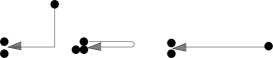
Figure 3: Illustration of two-link displacements.

Inclusion of the bent-links can enrich the angular distribution and recover parts of the continuum spherical harmonics that cannot be obtained from one-link displacements.

First, we classify the spatial degrees of freedom into a single IR of $O$ by forming linear combinations of the elemental operators of Eq. (51). The overall spatial IR $\Lambda$ and row $\lambda$ are determined by the direct product of the two spatial displacements ${\cal D}_{\lambda_{1}}^{\Lambda_{1}}$ and ${\cal D}_{\lambda_{2}}^{\Lambda_{2}}$ with appropriate Clebsch-Gordan coefficients,

$$\sum_{\lambda_{1},\lambda_{2}}C\left({\footnotesize\begin{array}[]{ccc}\Lambda&\Lambda_{1}&\Lambda_{2}\\ \lambda&\lambda_{1}&\lambda_{2}\end{array}}\right){\cal D}^{\Lambda_{2}}_{\lambda_{2}}{\cal D}^{\Lambda_{1}}_{\lambda_{1}}.$$ (52)

A particular example is instructive. Suppose one chooses ${\cal D}_{\lambda_{1}}^{\Lambda_{1}}$ to belong to the $T_{1}$ IR, and ${\cal D}_{\lambda_{2}}^{\Lambda_{2}}$ to belong to the $E$ IR and desires the overall spatial IR to be $T_{1}$. Then Eq.(52) is used with Clebsch-Gordan coefficients from the $E\otimes T_{1}$ table in Appendix D, which gives

$$\hat{\hat{T}}_{1}^{1} \sim {1\over 2}\hat{E}^{1}\times\hat{T}_{1}^{1}+{\sqrt{3}\over 2}\hat{E}^{2}\times\hat{T}_{1}^{3},$$

$$\hat{\hat{T}}_{1}^{2} \sim -\hat{E}^{1}\times\hat{T}_{1}^{2},$$

$$\hat{\hat{T}}_{1}^{3} \sim {1\over 2}\hat{E}^{1}\times\hat{T}_{1}^{3}+{\sqrt{3}\over 2}\hat{E}^{2}\times\hat{T}_{1}^{1}.$$

In this way the two-link operator is determined so that its spatial part transforms according to a particular IR (in this case $T_{1}$). Once the overall spatial IR is obtained, Clebsch-Gordan coefficients for the direct products of the overall spatial IR and a selected spinorial IR are used to form an operator that overall transforms irreducibly according to $G_{1},H$, or $G_{2}$. Because the spatial IR in the example above is $T_{1}$, which has been considered already in the construction of one-link operators, Table 10 provides the result. The only change is to use the $T_{1}$ distribution of two-link displacements in place of the $T_{1}$ distribution of one-link displacements. The use of Clebsch-Gordan coefficients of the cubic group has reduced the problem of finding IRs of two-link baryon operators to the already solved problem of finding one-link baryon operators.

However, new possibilities exist with the two-link displacements. One can form the $A_{2}$ and $T_{2}$ spatial IRs that did not appear in the one-link construction. This construction is straightforward but is omitted from this paper except to note that two-link $A_{2}$ and $T_{2}$ lattice harmonics correspond to the spherical harmonics shown in Table 2.

Proceeding in this fashion, one may construct multi-link baryon operators

$${\cal D}^{(3)\Lambda_{n}}_{\lambda_{n}}\cdot\cdot\cdot{\cal D}^{(3)\Lambda_{2}}_{\lambda_{2}}{\cal D}^{(3)\Lambda_{1}}_{\lambda_{1}}\overline{b}^{f_{1}f_{2}f_{3}}_{\mu_{1}\mu_{2}\mu_{3}}({\bf x})\equiv$$

$$\epsilon_{abc}\overline{q}^{af_{1}}_{\mu_{1}}({\bf x})\overline{q}^{bf_{2}}_{\mu_{2}}({\bf x})\left[{\cal D}_{\lambda_{n}}^{\Lambda_{n}}\cdot\cdot\cdot{\cal D}_{\lambda_{2}}^{\Lambda_{2}}{\cal D}_{\lambda_{1}}^{\Lambda_{1}}\overline{q}^{f_{3}}_{\mu_{3}}({\bf x})\right]^{c},$$ (53)

that involve $n$-site displacements in space allowing a quark to be displaced over a finer angular distribution so as to yield higher rank spherical harmonics. The reduction procedure is essentially the same as for the two-link case, except that multiple direct products of spatial IRs are used.

IV.5 One-link displacements applied to two different quarks

Consider an operator with one-link displacements applied to two different quarks in the following way,

$${\cal D}^{(1\pm 2)\Lambda_{2}}_{\lambda_{2}}{\cal D}^{(3)\Lambda_{1}}_{\lambda_{1}}\overline{b}^{f_{1}f_{2}f_{3}}_{\mu_{1}\mu_{2}\mu_{3}}\equiv$$

$${\epsilon_{abc}\over\sqrt{2}}\left[\left({\cal D}_{\lambda_{2}}^{\Lambda_{2}}\overline{q}^{f_{1}}_{\mu_{1}}\right)^{a}\overline{q}^{bf_{2}}_{\mu_{2}}\pm\overline{q}^{af_{1}}_{\mu_{1}}\left({\cal D}_{\lambda_{2}}^{\Lambda_{2}}\overline{q}^{f_{2}}_{\mu_{2}}\right)^{b}\right]\left({\cal D}_{\lambda_{1}}^{\Lambda_{1}}\overline{q}^{f_{3}}_{\mu_{3}}\right)^{c},$$ (54)

where ${\cal D}^{(1\pm 2)\Lambda}_{\lambda}$ indicates that the first two quark fields are symmetric or antisymmetric with respect to exchange of their spatial dependencies,

$${\cal D}^{(1\pm 2)\Lambda}_{\lambda}={1\over\sqrt{2}}\left({\cal D}^{(1)\Lambda}_{\lambda}\pm{\cal D}^{(2)\Lambda}_{\lambda}\right).$$ (55)

We refer to ${\cal D}^{(1+2)\Lambda}_{\lambda}$ as space-symmetric and to ${\cal D}^{(1-2)\Lambda}_{\lambda}$ as space-antisymmetric combinations of displacements. The symmetry of the spatial displacements must be taken into account in the overall antisymmetry of operators in order to identify the symmetry of Dirac indices that produces nonvanishing operators.

For the case of MA isospin nucleon operators with one-link displacements applied to two quarks, we obtain

$${\cal D}^{(1\pm 2)\Lambda_{2}}_{\lambda_{2}}{\cal D}^{(3)\Lambda_{1}}_{\lambda_{1}}\overline{N}^{\rm(MA)}_{\mu_{1}\mu_{2}\mu_{3}}$$ (56)

$$= \epsilon_{abc}{1\over 2}\left({\cal D}_{\lambda_{2}}^{\Lambda_{2}}\overline{u}^{a}_{\mu_{1}}\overline{d}^{b}_{\mu_{2}}-{\cal D}_{\lambda_{2}}^{\Lambda_{2}}\overline{d}^{a}_{\mu_{1}}\overline{u}^{b}_{\mu_{2}}\right)\left({\cal D}_{\lambda_{1}}^{\Lambda_{1}}\overline{u}_{\mu_{3}}\right)^{c}$$

$$\pm \epsilon_{abc}{1\over 2}\left(\overline{u}^{a}_{\mu_{1}}{\cal D}_{\lambda_{2}}^{\Lambda_{2}}\overline{d}^{b}_{\mu_{2}}-\overline{d}^{a}_{\mu_{1}}{\cal D}_{\lambda_{2}}^{\Lambda_{2}}\overline{u}^{b}_{\mu_{2}}\right)\left({\cal D}_{\lambda_{1}}^{\Lambda_{1}}\overline{u}_{\mu_{3}}\right)^{c},~{}$$

and the following relation between spatial symmetry of displacements and the symmetry of Dirac indices holds

$${\cal D}^{(1+2)\Lambda_{2}}_{\lambda_{2}}{\cal D}^{(3)\Lambda_{1}}_{\lambda_{1}}\overline{N}^{\rm(MA)}_{\mu_{1}\mu_{2}\mu_{3}}\rightarrow\rm{~{}~{}A,~{}MA~{}Dirac~{}indices}$$

$${\cal D}^{(1-2)\Lambda_{2}}_{\lambda_{2}}{\cal D}^{(3)\Lambda_{1}}_{\lambda_{1}}\overline{N}^{\rm(MA)}_{\mu_{1}\mu_{2}\mu_{3}}\rightarrow\rm{~{}~{}S,~{}MS~{}Dirac~{}indices}.$$ (57)

Because of symmetry, the operators of Eq. (56) with MA Dirac indices and those with MS Dirac indices are identical.

Group theoretically, rotations of operators with one-link displacements applied to two different quarks are the same as those of two-link operators. Therefore the reduction to IRs is exactly the same as for the two-link case. First use the Clebsch-Gordan coefficients to obtain an IR for the product of two displacements, and second use the Clebsch-Gordan coefficients for the direct product of spatial and spinorial IRs to obtain operators corresponding to overall IRs. The only additional step is to determine the allowed symmetries of Dirac indices such that the operator is antisymmetric under simultaneous exchange of displacements, flavors, colors, and Dirac indices.

V Summary

The constructions given in this paper provide a variety of quasi-local and nonlocal three-quark operators for use as zero-momentum baryon interpolating field operators in lattice QCD simulations. All operators are categorized into the double-valued IRs of the octahedral group $O^{D}_{h}$, they have definite parities and they are gauge invariant. Operators correspond as closely as possible to the continuum $|Jm\rangle$ IRs and they should be useful for spectroscopy and for applications that require baryons with a definite spin projection.

Complete sets of quasi-local operators are presented in Section III for each baryon. These quasi-local constructions provide templates for the Dirac indices that should be used to construct nonlocal operators. Nonlocal operators are developed in Section IV based on adding combinations of one-link displacements to one or more quarks. By use of the building blocks given in this paper, a variety of additional operators can be constructed by 1) using the Clebsch-Gordan series to form overall IRs of the spatial distribution, and 2) combining the spatial IRs with IRs of Dirac indices to form operators corresponding to overall IRs. Identification of the correct symmetry of Dirac indices is straightforward when space-symmetric or space-antisymmetric combinations of displacements are used.

Reference Sato04 has demonstrated numerically that our quasi-local and one-link operators are orthogonal in the sense of Eq. (15), i.e., a correlation function vanishes if sink and source operators belong to different IRs and rows. For calculations of baryon masses, one should select source operators within a fixed IR and row from the various tables. Using operators from different embeddings of the IR and row, matrices of correlation functions may be calculated and mass spectra extracted. Correlation matrices can be made hermitian by including a $\gamma_{4}$ matrix for each quark in the source operator. Operators from our tables have the form $\overline{B}^{\Lambda,k}_{\lambda}=c^{(\Lambda,\lambda,k)}_{\mu_{1}\mu_{2}\mu_{3}}\overline{B}_{\mu_{1}\mu_{2}\mu_{3}}$, where $\overline{B}_{\mu_{1}\mu_{2}\mu_{3}}$ is an elemental baryon operator and a summation over repeated indices is understood. A hermitian matrix of correlation functions can be calculated in following way,

$$C^{\prime(\Lambda)}_{kk^{\prime}}(t)=\sum_{x}\left<0\right|TB^{\Lambda,k}_{\lambda}({\bf x},t)\overline{B}^{\Lambda,k^{\prime}}_{\lambda}(0)\left|0\right>\Gamma_{4}$$

$$=\sum_{x}c^{(\Lambda,\lambda,k)*}_{\mu_{1}\mu_{2}\mu_{3}}c^{(\Lambda,\lambda,k^{\prime})}_{\mu_{1}^{\prime}\mu_{2}^{\prime}\mu_{3}^{\prime}}\left<0\right|TB_{\mu_{1}\mu_{2}\mu_{3}}({\bf x},t)\overline{B}_{\nu_{1}\nu_{2}\nu_{3}}(0)\left|0\right>$$

$$~{}~{}~{}\times\gamma_{4\nu_{1}\mu_{1}^{\prime}}\gamma_{4\nu_{2}\mu_{2}^{\prime}}\gamma_{4\nu_{3}\mu_{3}^{\prime}}.$$ (58)

Exploratory calculations for baryon spectra along this line have been reported in Ref. Basak04 . For a given baryon, the dimension of the matrix of correlation functions depends on the choices that are made for spatial distributions (quasi-local, one-link, two-link, etc.) and the overall IR. For nucleon operators with quasi-local and one-link displacements, 23 $G_{1g}$ operators, 28 $H_{g}$ operators, and 7 $G_{2g}$ operators are available as shown in Table 13. The numbers of operators in each IR and row can be extended without limit by using two-link and three-link operators and by using different choices of smearing.

Table 13: Available numbers of nucleon operators with quasi-local and with one-link displacements for $G_{1g}$ row 1, $G_{2g}$ row 1, and $H_{g}$ row 1. The numbers of ungerade operators are exactly the same. The $T_{1}$ $\overline{N}^{\rm(MS)}$ operators are omitted because after a projection to zero total momentum they are equivalent to the $T_{1}$ $\overline{N}^{\rm(MA)}$ operators.

Type	Eq.	Table	$G_{1g}$	$H_{g}$	$G_{2g}$
quasi-local	16	6	3	1	0
one-link $A_{1}$	43	8	4	1	0
one-link $E$	43	11, 8	1	5	1
one-link $T_{1}$	43	10, 8	5	6	1
one-link $A_{1}$	45	9	4	3	0
one-link $E$	45	11, 9	3	7	3
one-link $T_{1}$	45	10, 9	3	5	2
total			23	28	7

Appendix A Dirac matrices

Various conventions for the Dirac matrices are useful. Each is related by a unitary transformation to the Dirac-Pauli representation as follows,

$$\gamma_{\mu}=U\gamma_{\mu}^{\rm(DP)}U^{{\dagger}},$$ (59)

where

$$\gamma_{j}^{\rm(DP)}=\left(\begin{array}[]{cc}0&-i\sigma_{j}\\ i\sigma_{j}&0\end{array}\right),~{}~{}\gamma_{4}^{\rm(DP)}=\left(\begin{array}[]{cc}1&0\\ 0&-1\end{array}\right).$$ (60)

The unitary matrix that generates the Weyl convention is

$$U^{(W)}=\frac{1+\gamma^{\rm(DP)}_{5}\gamma^{\rm(DP)}_{4}}{\sqrt{2}},$$ (61)

and the unitary transformation that generates the DeGrand-Rossi convention is

$$U^{\rm(DR)}=\frac{-i\gamma^{\rm(DP)}_{2}+\gamma^{\rm(DP)}_{1}\gamma^{\rm(DP)}_{3}}{\sqrt{2}}.$$ (62)

A quark field expressed in terms of the Dirac-Pauli representation may be re-expressed in the Degrand-Rossi convention, for example, by

$$q^{\rm(DP)}_{\mu}=\left(U^{\rm(DR){\dagger}}\right)_{\mu\nu}q^{\rm(DR)}_{\nu}.$$ (63)

In order to display the spin and $\rho$-parity of fields in a transparent way, we employ spin $s$ subscripts and $\rho$ superscripts in place of the four Dirac components $\mu$ = 1, 2, 3 and 4 of each quark field in the Dirac-Pauli representation as shown in Table 5.

This encoding of the Dirac indices is based on the $SU(2)\otimes SU(2)$ representation of the Dirac matrices, where the first $SU(2)$ is generated by 2$\times$2 Pauli matrices for $\rho$-spin,

$$\rho_{1}=\left(\begin{array}[]{cc}0&1\\ 1&0\end{array}\right),\rho_{2}=\left(\begin{array}[]{cc}0&-i\\ i&0\end{array}\right),\rho_{3}=\left(\begin{array}[]{cc}1&0\\ 0&-1\end{array}\right),$$ (70)

and the second $SU(2)$ is generated by the Pauli matrices for ordinary spin,

$$\sigma_{1}=\left(\begin{array}[]{cc}0&1\\ 1&0\end{array}\right),\sigma_{2}=\left(\begin{array}[]{cc}0&-i\\ i&0\end{array}\right),\sigma_{3}=\left(\begin{array}[]{cc}1&0\\ 0&-1\end{array}\right).$$ (77)

The $2\times 2$ identity matrices for $\rho$-spin and ordinary spin are

$$\rho_{4}=\sigma_{4}=\left(\begin{array}[]{cc}1&0\\ 0&1\end{array}\right).$$ (80)

In terms of these sets of 2$\times$2 matrices, the 4$\times$4 Dirac-Pauli matrices are expressed as direct products of $\rho$-spin matrices and $s$-spin matrices as follows,

$$I = \rho_{4}\otimes\sigma_{4},$$

$$\gamma_{4} = \rho_{3}\otimes\sigma_{4},$$

$$\gamma_{5} = \rho_{1}\otimes\sigma_{4},$$

$$\gamma_{5}\gamma_{4} = -i\rho_{2}\otimes\sigma_{4},$$

$$\gamma_{5}\gamma_{k} = i\rho_{3}\otimes\sigma_{k},$$

$$\gamma_{k} = \rho_{2}\otimes\sigma_{k},$$

$$\sigma_{4k} = \rho_{1}\otimes\sigma_{k},$$

$$\sigma_{kl} = -\epsilon_{klm}\rho_{4}\otimes\sigma_{m},$$ (81)

where $k,l$, and $m$ take the values 1, 2 and 3.

Appendix B Symmetry of three Dirac fields

The Dirac indices categorized in each Young tableau in Fig. 2 should be further reduced into $G_{1}$ or $H$ IRs for the purpose of operator construction. (There is no $G_{2}$ IR with three Dirac spinors.) Decomposition of the Dirac index into $\rho$-parity and ordinary two-component spin ($s$-spin) simplifies this process.

The S (totally symmetric), MS (mixed-symmetric), and MA (mixed-antisymmetric) combinations of three $s$-spins are defined as follows.

$${\rm S} : \left|+++\right>;{\left|++-\right>+\left|+-+\right>+\left|-++\right>\over\sqrt{3}};$$ (82)

$${\left|+--\right>+\left|-+-\right>+\left|--+\right>\over\sqrt{3}};\left|---\right>.$$

$${\rm MS} : {1\over\sqrt{6}}\left(2\left|++-\right>-\left|+-+\right>-\left|-++\right>\right);$$ (83)

$$-{1\over\sqrt{6}}\left(2\left|--+\right>-\left|-+-\right>-\left|+--\right>\right).$$

$${\rm MA} : {1\over\sqrt{2}}\left(\left|+-+\right>-\left|-++\right>\right);{1\over\sqrt{2}}\left(\left|+--\right>-\left|-+-\right>\right).$$ (84)

The four states in Eq. (82) are $\left|J,m\right>=$ $\left|{3\over 2}{3\over 2}\right>$, $\left|{3\over 2}{1\over 2}\right>$, $\left|{3\over 2}-{1\over 2}\right>$, and $\left|{3\over 2}-{3\over 2}\right>$ respectively. The two states in Eq. (83) are $\left|{1\over 2}{1\over 2}\right>$ and $\left|{1\over 2}-{1\over 2}\right>$ while the two states in Eq. (84) are also $\left|{1\over 2}{1\over 2}\right>$ and $\left|{1\over 2}-{1\over 2}\right>$. All these states are orthogonal to one other. Because S states in Eq. (82) span total spin 3/2, they are the bases of an $H$ IR (no matter which $\rho$’s are involved in making up the Dirac indices). The MS and MA states in Eq. (83, 84) span total spin 1/2, so they are the bases of $G_{1}$ IRs.

Products of three $\rho$-spins are categorized in exactly the same way. The $\rho$-parity is given by the product $\rho_{1}\rho_{2}\rho_{3}$. Direct products of states of three $\rho$-spins and states of three $s$-spins are simple when they are expressed in the bases of S, MS, and MA. For instance, ${\rm MA}_{\rho}\otimes{\rm S}_{s}$ with subscripts denoting $\rho$-spin and $s$-spin describes eight states, four of which have positive $\rho$-parity, and four of which have negative $\rho$-parity. The four states of each $\rho$-parity span $H$ IRs because IRs of $O^{D}$ are determined only by the $s$-spins. The direct product of ${\rm MA}_{\rho}\otimes{\rm S}_{s}$, with $\left|{1\over 2},-{1\over 2}\right>_{\rho}$ and $\left|{3\over 2},{1\over 2}\right>_{s}$ is written as

$${\left|+--\right>_{\rho}-\left|-+-\right>_{\rho}\over\sqrt{2}}\otimes{\left|++-\right>_{s}+\left|+-+\right>_{s}+\left|-++\right>_{s}\over\sqrt{3}}.$$

By evaluating the direct product one obtains

$${1\over\sqrt{6}}\left(\left|{}^{+--}_{++-}\right>+\left|{}^{+--}_{+-+}\right>+\left|{}^{+--}_{-++}\right>-\left|{}^{-+-}_{++-}\right>-\left|{}^{-+-}_{+-+}\right>-\left|{}^{-+-}_{-++}\right>\right),$$

where the notation $\left|{}^{\rho_{1}\rho_{2}\rho_{3}}_{s_{1}s_{2}s_{3}}\right>$ is used. In terms of the $\left|\mu_{1}\mu_{2}\mu_{3}\right>$ notation, it becomes

$${1\over\sqrt{6}}\left(\left|134\right>+\left|143\right>+\left|233\right>-\left|314\right>-\left|323\right>-\left|413\right>\right),$$

where the Dirac indices $\mu_{i}=1,2,3,4$ are defined in Dirac-Pauli representation of Dirac $\gamma$ matrices. The translation of $\mu$ to $(\rho,s)$ is given in Table 5. It is clear that the obtained Dirac indices are antisymmetric under exchange of first two labels but not totally antisymmetric. Thus, we denote ${\rm MA}_{\rho}\otimes{\rm S}_{s}={\rm MA}_{\rm Dirac}$. The nucleon operator that follows from this example is labeled as $H_{g}$, row 2 in Table 6.

From such considerations one obtains Table 14, which provides the relations of Dirac index symmetries (abbreviated as “Dirac sym” in the table) to IRs of Dirac indices, and direct products of $\rho$-spins and $s$-spins.

Table 14: Relation among Dirac spin symmetry, IR, and the direct product of $\rho$-spins and $s$-spins.

Dirac sym	IR	emb	$\rho\otimes s$
${\rm S}_{\rm Dirac}$	$G_{1}$	1	${\rm MA}_{\rho}\otimes{\rm MA}_{s}\oplus{\rm MS}_{\rho}\otimes{\rm MS}_{s}$
	$H$	1,2	${\rm S}_{\rho}\otimes{\rm S}_{s}$
${\rm MS}_{\rm Dirac}$	$G_{1}$	1,2	${\rm S}_{\rho}\otimes{\rm MS}_{s}$
		3	${\rm MA}_{\rho}\otimes{\rm MA}_{s}\ominus{\rm MS}_{\rho}\otimes{\rm MS}_{s}$
	$H$	1	${\rm MS}_{\rho}\otimes{\rm S}_{s}$
${\rm MA}_{\rm Dirac}$	$G_{1}$	1,2	${\rm S}_{\rho}\otimes{\rm MA}_{s}$
		3	${\rm MA}_{\rho}\otimes{\rm MS}_{s}\oplus{\rm MS}_{\rho}\otimes{\rm MA}_{s}$
	$H$	1	${\rm MA}_{\rho}\otimes{\rm S}_{s}$
${\rm A}_{\rm Dirac}$	$G_{1}$	1,2	${\rm MA}_{\rho}\otimes{\rm MS}_{s}\ominus{\rm MS}_{\rho}\otimes{\rm MA}_{s}$

Note that ${\rm MA}_{\rho}\otimes{\rm MA}_{s}$ and ${\rm MS}_{\rho}\otimes{\rm MS}_{s}$ both have a mixture of ${\rm S}_{\rm Dirac}$ and ${\rm MS}_{\rm Dirac}$. One can easily see that addition of a state from ${\rm MA}_{\rho}\otimes{\rm MA}_{s}$, say $G_{1g}$, row 1, and a state from ${\rm MS}_{\rho}\otimes{\rm MS}_{s}$ of the same $G_{1g}$, row 1 yields a pure ${\rm S}_{\rm Dirac}$ state. The subtraction of the states yields a pure ${\rm MS}_{\rm Dirac}$ state. Similarly, ${\rm MA}_{\rho}\otimes{\rm MS}_{s}$ and ${\rm MS}_{\rho}\otimes{\rm MA}_{s}$ have a mixture of ${\rm MA}_{\rm Dirac}$ and ${\rm A}_{\rm Dirac}$. A pure ${\rm MA}_{\rm Dirac}$ is obtained by addition of states from ${\rm MA}_{\rho}\otimes{\rm MS}_{s}$ and ${\rm MS}_{\rho}\otimes{\rm MA}_{s}$ and a pure ${\rm A}_{\rm Dirac}$ is obtained by subtraction of states from ${\rm MA}_{\rho}\otimes{\rm MS}_{s}$ and ${\rm MS}_{\rho}\otimes{\rm MA}_{s}$. The third column of Table 14 shows an embedding that has a connection to Table 15 in a self-explanatory way.

Table 15: IRs of S, MS combinations of Dirac indices for three quark states in Dirac-Pauli representation. The first entry of MS table reads $2\overline{q}^{f_{1}}_{1}\overline{q}^{f_{2}}_{1}\overline{q}^{f_{3}}_{2}-\overline{q}^{f_{1}}_{1}\overline{q}^{f_{2}}_{2}\overline{q}^{f_{3}}_{1}-\overline{q}^{f_{1}}_{2}\overline{q}^{f_{2}}_{1}\overline{q}^{f_{3}}_{1}$ for the $G_{1g}$, embedding 1, row 1 local operator.

$\Lambda$	$k$	$\lambda$	S Dirac indices $\mu_{1}\mu_{2}\mu_{3}$
$G_{1g}$	1	1	$-2(332+323+233)+341+431+314+413+134+143$
		2	$2(144+414+441)-234-342-423-243-324-432$
$G_{1u}$	1	1	$2(114+141+411)-123-213-132-231-321-312$
		2	$-2(223+232+322)+214+124+241+142+421+412$
$H_{g}$	1	1	$111$
		2	$112+121+211$
		3	$122+212+221$
		4	$222$
	2	1	$133+313+331$
		2	$233+323+332+134+341+413+143+431+314$
		3	$144+414+441+234+342+423+243+432+324$
		4	$244+424+442$
$H_{u}$	1	1	$113+131+311$
		2	$411+141+114+312+123+231+321+213+132$
		3	$322+232+223+412+124+241+421+214+142$
		4	$224+242+422$
	2	1	$333$
		2	$334+343+433$
		3	$344+434+443$
		4	$444$
$\Lambda$	$k$	$\lambda$	MS Dirac indices $\mu_{1}\mu_{2}\mu_{3}$
$G_{1g}$	1	1	$2(112)-121-211$
		2	$-2(221)+212+122$
	2	1	$2(332+314+134)-341-323-143-431-413-233$
		2	$-2(441+423+243)+432+414+234+342+324+144$
	3	1	$-2(332+413+143)+323+233+134+314+341+431$
		2	$2(441+324+234)-414-144-243-423-432-342$
$G_{1u}$	1	1	$2(114+132+312)-123-141-321-213-231-411$
		2	$-2(223+241+421)+214+232+412+124+142+322$
	2	1	$2(334)-343-433$
		2	$-2(443)+434+344$
	3	1	$2(114+231+321)-141-411-312-132-123-213$
		2	$-2(223+142+412)+232+322+421+241+214+124$
$H_{g}$	1	1	$-2(331)+313+133$
		2	$-2(332+341+431)+314+134+323+143+413+233$
		3	$-2(342+432+441)+324+144+414+234+423+243$
		4	$-2(442)+424+244$
$H_{u}$	1	1	$2(113)-131-311$
		2	$2(114+123+213)-132-312-141-321-231-411$
		3	$2(124+214+223)-142-322-232-412-241-421$
		4	$2(224)-242-422$

Table 16: IRs of MA, A combinations of Dirac indices for three-quark states in Dirac-Pauli representation. The caption in Table 15 describes how to read this table.

$\Lambda$	$k$	$\lambda$	MA Dirac indices $\mu_{1}\mu_{2}\mu_{3}$
$G_{1g}$	1	1	$121-211$
		2	$122-212$
	2	1	$143-233+323-413+341-431$
		2	$144-234+324-414+342-432$
	3	1	$-233+323+134-314-341+431$
		2	$-414+144-243+423+432-342$
$G_{1u}$	1	1	$123-213+141-231+321-411$
		2	$124-214+142-232+322-412$
	2	1	$343-433$
		2	$344-434$
	3	1	$-141+411-312+132+123-213$
		2	$232-322+421-241-214+124$
$H_{g}$	1	1	$133-313$
		2	$134-314+143-323+233-413$
		3	$144-324+234-414+243-423$
		4	$244-424$
$H_{u}$	1	1	$131-311$
		2	$132-312+141-321+231-411$
		3	$142-322+232-412+241-421$
		4	$242-422$
$\Lambda$	$k$	$\lambda$	A Dirac indices $\mu_{1}\mu_{2}\mu_{3}$
$G_{1g}$	1	1	$134-314+341-431+413-143$
		2	$234-324+342-432+423-243$
$G_{1u}$	1	1	$-123+213-231+321-312+132$
		2	$-124+214-241+421-412+142$

Explicit combinations of Dirac indices $\mu_{1}\mu_{2}\mu_{3}$ are given in Tables 15 and 16. Table 15 contains all S and MS combinations of three Dirac indices, assigning each to an IR ( $G_{1g/u}$ or $H_{g/u}$), embedding, and row. Table 16 contains all MA and A combinations of three Dirac indices in a similar way.

Appendix C Relations of $N_{\mu_{1}\mu_{2}\mu_{3}}$ to commonly used nucleon operators

Various groups have performed lattice simulations using the following two interpolating fields for a nucleon:

$$\chi^{1/2}_{1} = \left(u^{T}C\gamma_{5}d\right)u,$$ (85)

$$\chi^{1/2}_{2} = \left(u^{T}Cd\right)\gamma_{5}u,$$ (86)

where spacetime arguments are omitted. Matrix $C$ is a charge-conjugation operator, defined by $C=\gamma_{4}\gamma_{2}$. Each of these four-component operators corresponds to a $G_{1}$ IR and may be written in terms of $\overline{\Psi}^{\Lambda,k}_{S,S_{z}}$. Positive and negative $\rho$-parity parts of $\chi^{1/2}_{1}$ are projected in Dirac-Pauli representation as follows,

$${1+\gamma_{4}\over 2}\chi^{1/2}_{1} = \left(\begin{tabular}[]{c}$-N_{121}-N_{341}$\\ $-N_{122}-N_{342}$\end{tabular}\right)$$ (89)

$${1-\gamma_{4}\over 2}\chi^{1/2}_{1} = \left(\begin{tabular}[]{c}$-N_{123}-N_{343}$\\ $-N_{124}-N_{344}$\end{tabular}\right)$$ (92)

The upper component corresponds to $S_{z}=+1/2$. Similarly $\chi^{1/2}_{2}$ can be projected to operators of definite $\rho$-parity,

$${1+\gamma_{4}\over 2}\chi^{1/2}_{2} = \left(\begin{tabular}[]{c}$N_{143}-N_{233}$\\ $N_{144}-N_{234}$\end{tabular}\right)$$ (96)

$${1-\gamma_{4}\over 2}\chi^{1/2}_{2} = \left(\begin{tabular}[]{c}$N_{141}-N_{231}$\\ $N_{142}-N_{232}$\end{tabular}\right)$$ (99)

. (100)

These results show how the components of $\chi_{1}^{1/2}$ and $\chi_{2}^{1/2}$ are related to operators defined in this paper.

Appendix D Clebsch-Gordan coefficients for the double octahedral group

The Clebsch-Gordan formula shows how an IR operator $\overline{\cal O}^{\Lambda}_{\lambda}$ may be built from linear combinations of direct products of other IR operators, $\overline{\cal O}^{\Lambda_{1}}_{\lambda_{1}}$ and $\overline{\cal O}^{\Lambda_{2}}_{\lambda_{2}}$,

$$\overline{\cal O}^{\Lambda}_{\lambda}=\sum_{\lambda_{1},\lambda_{2}}C\left({\footnotesize\begin{tabular}[]{ccc}$\Lambda$&$\Lambda_{1}$&$\Lambda_{2}$\\ $\lambda$&$\lambda_{1}$&$\lambda_{2}$\end{tabular}}\right)\overline{\cal O}^{\Lambda_{1}}_{\lambda_{1}}\overline{\cal O}^{\Lambda_{2}}_{\lambda_{2}},$$ (103)

where $\Lambda$ $(\Lambda_{i})$ and $\lambda$ $(\lambda_{i})$ denote IR and row, respectively. The notation $\overline{\cal O}^{\Lambda}_{\lambda}$ can refer to $\hat{A}_{1},\hat{A}_{2}^{\lambda},\hat{E}^{\lambda},\hat{T}_{1}^{\lambda},\hat{T}_{2}^{\lambda},\overline{\Psi}^{G_{1g}}_{\lambda},\overline{\Psi}^{G_{1u}}_{\lambda},\overline{\Psi}^{H_{g}}_{\lambda}$, or $\overline{\Psi}^{H_{u}}_{\lambda}$. See the comments in the paragraph above Eq. (41) for our phase convention for the coefficients.

A complete set of Clebsch-Gordan coefficients for the octahedral group using the basis vectors of Tables 2 and 4 is given here and in Ref. IkuroThesis . The version of this paper that was submitted for publication was shortened by omitting all but a selected subset of Clebsch-Gordan coefficients.

In each Clebsch-Gordan table, the resultant IR appearing on the left side of Eq. (103) is listed in the top row, and the two IRs appearing on the right side of Eq. (103) are listed in the left column. Table 17 explains how to read the coefficients in the Clebsch-Gordan tables in this appendix.

Table 17: Description for tables of Clebsch-Gordan coefficients. Squares of coefficients are listed together with their overall sign.

$\overline{\cal O}^{\Lambda_{1}}\otimes\overline{\cal O}^{\Lambda_{2}}$	$\overline{\cal O}^{\Lambda}_{\lambda}$
$\overline{\cal O}^{\Lambda_{1}}_{\lambda_{1}}\overline{\cal O}^{\Lambda_{2}}_{\lambda_{2}}$	$sgn\left[C\left({\footnotesize\begin{array}[]{ccc}\Lambda&\Lambda_{1}&\Lambda_{2}\\ \lambda&\lambda_{1}&\lambda_{2}\end{array}}\right)\right]\left|C\left({\footnotesize\begin{array}[]{ccc}\Lambda&\Lambda_{1}&\Lambda_{2}\\ \lambda&\lambda_{1}&\lambda_{2}\end{array}}\right)\right|^{2}$

$E\!\!\otimes\!T_{1}$	$T_{1}^{1}$	$T_{1}^{2}$	$T_{1}^{3}$	$T_{2}^{1}$	$T_{2}^{2}$	$T_{2}^{3}$
$E^{1}T_{1}^{1}$	1/4	0	0	3/4	0	0
$E^{1}T_{1}^{2}$	0	-1	0	0	0	0
$E^{1}T_{1}^{3}$	0	0	1/4	0	0	-3/4
$E^{2}T_{1}^{1}$	0	0	3/4	0	0	1/4
$E^{2}T_{1}^{2}$	0	0	0	0	-1	0
$E^{2}T_{1}^{3}$	3/4	0	0	-1/4	0	0

$E\!\!\otimes\!G_{1}$	$H^{1}$	$H^{2}$	$H^{3}$	$H^{4}$
$E^{1}G_{1}^{1}$	0	-1	0	0
$E^{1}G_{1}^{2}$	0	0	1	0
$E^{2}G_{1}^{1}$	0	0	0	-1
$E^{2}G_{1}^{2}$	1	0	0	0

$T_{1}\!\!\otimes\!G_{1}$	$G_{1}^{1}$	$G_{1}^{2}$	$H^{1}$	$H^{2}$	$H^{3}$	$H^{4}$
$T_{1}^{1}G_{1}^{1}$	0	0	1	0	0	0
$T_{1}^{1}G_{1}^{2}$	2/3	0	0	1/3	0	0
$T_{1}^{2}G_{1}^{1}$	-1/3	0	0	2/3	0	0
$T_{1}^{2}G_{1}^{2}$	0	1/3	0	0	2/3	0
$T_{1}^{3}G_{1}^{1}$	0	-2/3	0	0	1/3	0
$T_{1}^{3}G_{1}^{2}$	0	0	0	0	0	1

$E\!\!\otimes\!H$	$G_{1}^{1}$	$G_{1}^{2}$	$G_{2}^{1}$	$G_{2}^{2}$	$H^{1}$	$H^{2}$	$H^{3}$	$H^{4}$
$E^{1}H^{1}$	0	0	0	-1/2	1/2	0	0	0
$E^{1}H^{2}$	1/2	0	0	0	0	-1/2	0	0
$E^{1}H^{3}$	0	-1/2	0	0	0	0	-1/2	0
$E^{1}H^{4}$	0	0	1/2	0	0	0	0	1/2
$E^{2}H^{1}$	0	-1/2	0	0	0	0	1/2	0
$E^{2}H^{2}$	0	0	-1/2	0	0	0	0	1/2
$E^{2}H^{3}$	0	0	0	1/2	1/2	0	0	0
$E^{2}H^{4}$	1/2	0	0	0	0	1/2	0	0

$A_{2}\!\!\otimes\!E$	$E^{1}$	$E^{2}$
$A_{2}E^{1}$	0	-1
$A_{2}E^{2}$	1	0

$A_{2}\!\!\otimes\!T_{1}$	$T_{2}^{1}$	$T_{2}^{2}$	$T_{2}^{3}$
$A_{2}T_{1}^{1}$	0	0	-1
$A_{2}T_{1}^{2}$	0	-1	0
$A_{2}T_{1}^{3}$	1	0	0

$A_{2}\!\!\otimes\!T_{2}$	$T_{1}^{1}$	$T_{1}^{2}$	$T_{1}^{3}$
$A_{2}T_{2}^{1}$	0	0	-1
$A_{2}T_{2}^{2}$	0	1	0
$A_{2}T_{2}^{3}$	1	0	0

$A_{2}\!\!\otimes\!G_{1}$	$G_{2}^{1}$	$G_{2}^{2}$
$A_{2}G_{1}^{1}$	1	0
$A_{2}G_{1}^{2}$	0	1

$A_{2}\!\!\otimes\!G_{2}$	$G_{1}^{1}$	$G_{1}^{2}$
$A_{2}G_{2}^{1}$	1	0
$A_{2}G_{2}^{2}$	0	1

$A_{2}\!\!\otimes\!H$	$H^{1}$	$H^{2}$	$H^{3}$	$H^{4}$
$A_{2}H^{1}$	0	0	-1	0
$A_{2}H^{2}$	0	0	0	1
$A_{2}H^{3}$	1	0	0	0
$A_{2}H^{4}$	0	-1	0	0

$E\!\!\otimes\!E$	$A_{1}$	$A_{2}$	$E^{1}$	$E^{2}$
$E^{1}E^{1}$	1/2	0	1/2	0
$E^{1}E^{2}$	0	1/2	0	-1/2
$E^{2}E^{1}$	0	-1/2	0	-1/2
$E^{2}E^{2}$	1/2	0	-1/2	0

$E\!\!\otimes\!G_{2}$	$H^{1}$	$H^{2}$	$H^{3}$	$H^{4}$
$E^{1}G_{2}^{1}$	0	0	0	-1
$E^{1}G_{2}^{2}$	1	0	0	0
$E^{2}G_{2}^{1}$	0	1	0	0
$E^{2}G_{2}^{2}$	0	0	-1	0

$E\!\!\otimes\!T_{2}$	$T_{1}^{1}$	$T_{1}^{2}$	$T_{1}^{3}$	$T_{2}^{1}$	$T_{2}^{2}$	$T_{2}^{3}$
$E^{1}T_{2}^{1}$	3/4	0	0	1/4	0	0
$E^{1}T_{2}^{2}$	0	0	0	0	-1	0
$E^{1}T_{2}^{3}$	0	0	-3/4	0	0	1/4
$E^{2}T_{2}^{1}$	0	0	-1/4	0	0	-3/4
$E^{2}T_{2}^{1}$	0	-1	0	0	0	0
$E^{2}T_{2}^{1}$	1/4	0	0	-3/4	0	0

$T_{1}\!\!\otimes\!T_{1}$	$A_{1}$	$E^{1}$	$E^{2}$	$T_{1}^{1}$	$T_{1}^{2}$	$T_{1}^{3}$	$T_{2}^{1}$	$T_{2}^{2}$	$T_{2}^{3}$
$T_{1}^{1}T_{1}^{1}$	0	0	1/2	0	0	0	0	1/2	0
$T_{1}^{1}T_{1}^{2}$	0	0	0	1/2	0	0	1/2	0	0
$T_{1}^{1}T_{1}^{3}$	1/3	1/6	0	0	1/2	0	0	0	0
$T_{1}^{2}T_{1}^{1}$	0	0	0	-1/2	0	0	1/2	0	0
$T_{1}^{2}T_{1}^{2}$	-1/3	2/3	0	0	0	0	0	0	0
$T_{1}^{2}T_{1}^{3}$	0	0	0	0	0	1/2	0	0	1/2
$T_{1}^{3}T_{1}^{1}$	1/3	1/6	0	0	-1/2	0	0	0	0
$T_{1}^{3}T_{1}^{2}$	0	0	0	0	0	-1/2	0	0	1/2
$T_{1}^{3}T_{1}^{3}$	0	0	1/2	0	0	0	0	-1/2	0

$T_{\!1}\!\!\otimes\!H$	$G_{1}^{1}$	$G_{1}^{2}$	$G_{2}^{1}$	$G_{2}^{2}$	$H^{1}$	$H^{2}$	$H^{3}$	$H^{4}$	$H^{1}$	$H^{2}$	$H^{3}$	$H^{4}$
$T_{1}^{1}H^{1}$	0	0	1/6	0	0	0	0	0	0	0	0	-5/6
$T_{1}^{1}H^{2}$	0	0	0	-1/2	-2/5	0	0	0	1/10	0	0	0
$T_{1}^{1}H^{3}$	1/6	0	0	0	0	-8/15	0	0	0	-3/10	0	0
$T_{1}^{1}H^{4}$	0	1/2	0	0	0	0	-2/5	0	0	0	1/10	0
$T_{1}^{2}H^{1}$	0	0	0	-1/3	3/5	0	0	0	1/15	0	0	0
$T_{1}^{2}H^{2}$	-1/3	0	0	0	0	1/15	0	0	0	-3/5	0	0
$T_{1}^{2}H^{3}$	0	-1/3	0	0	0	0	-1/15	0	0	0	3/5	0
$T_{1}^{2}H^{4}$	0	0	-1/3	0	0	0	0	-3/5	0	0	0	-1/15
$T_{1}^{3}H^{1}$	1/2	0	0	0	0	2/5	0	0	0	-1/10	0	0
$T_{1}^{3}H^{2}$	0	1/6	0	0	0	0	8/15	0	0	0	3/10	0
$T_{1}^{3}H^{3}$	0	0	-1/2	0	0	0	0	2/5	0	0	0	-1/10
$T_{1}^{3}H^{4}$	0	0	0	1/6	0	0	0	0	5/6	0	0	0

$T_{1}\!\!\otimes\!T_{2}$	$A_{2}$	$E^{1}$	$E^{2}$	$T_{1}^{1}$	$T_{1}^{2}$	$T_{1}^{3}$	$T_{2}^{1}$	$T_{2}^{2}$	$T_{2}^{3}$
$T_{1}^{1}T_{2}^{1}$	1/3	0	1/6	0	0	0	0	-1/2	0
$T_{1}^{1}T_{2}^{2}$	0	0	0	0	0	1/2	0	0	1/2
$T_{1}^{1}T_{2}^{3}$	0	1/2	0	0	-1/2	0	0	0	0
$T_{1}^{2}T_{2}^{1}$	0	0	0	1/2	0	0	1/2	0	0
$T_{1}^{2}T_{2}^{2}$	1/3	0	-2/3	0	0	0	0	0	0
$T_{1}^{2}T_{2}^{3}$	0	0	0	0	0	1/2	0	0	-1/2
$T_{1}^{3}T_{2}^{1}$	0	-1/2	0	0	-1/2	0	0	0	0
$T_{1}^{3}T_{2}^{2}$	0	0	0	-1/2	0	0	1/2	0	0
$T_{1}^{3}T_{2}^{3}$	-1/3	0	-1/6	0	0	0	0	-1/2	0

$T_{1}\!\!\otimes\!G_{2}$	$G_{2}^{1}$	$G_{2}^{2}$	$H^{1}$	$H^{2}$	$H^{3}$	$H^{4}$
$T_{1}^{1}G_{2}^{1}$	0	0	0	0	-1	0
$T_{1}^{1}G_{2}^{2}$	2/3	0	0	0	0	1/3
$T_{1}^{2}G_{2}^{1}$	-1/3	0	0	0	0	2/3
$T_{1}^{2}G_{2}^{2}$	0	1/3	2/3	0	0	0
$T_{1}^{3}G_{2}^{1}$	0	-2/3	1/3	0	0	0
$T_{1}^{3}G_{2}^{2}$	0	0	0	-1	0	0

$T_{2}\!\!\otimes\!T_{2}$	$A_{1}$	$E^{1}$	$E^{2}$	$T_{1}^{1}$	$T_{1}^{2}$	$T_{1}^{3}$	$T_{2}^{1}$	$T_{2}^{2}$	$T_{2}^{3}$
$T_{2}^{1}T_{2}^{1}$	0	0	-1/2	0	0	0	0	-1/2	0
$T_{2}^{1}T_{2}^{2}$	0	0	0	0	0	-1/2	0	0	-1/2
$T_{2}^{1}T_{2}^{3}$	1/3	1/6	0	0	-1/2	0	0	0	0
$T_{2}^{2}T_{2}^{1}$	0	0	0	0	0	1/2	0	0	-1/2
$T_{2}^{2}T_{2}^{2}$	1/3	-2/3	0	0	0	0	0	0	0
$T_{2}^{2}T_{2}^{3}$	0	0	0	1/2	0	0	1/2	0	0
$T_{2}^{3}T_{2}^{1}$	1/3	1/6	0	0	1/2	0	0	0	0
$T_{2}^{3}T_{2}^{2}$	0	0	0	-1/2	0	0	1/2	0	0
$T_{2}^{3}T_{2}^{3}$	0	0	-1/2	0	0	0	0	1/2	0

$T_{2}\!\!\otimes\!G_{1}$	$G_{2}^{1}$	$G_{2}^{2}$	$H^{1}$	$H^{2}$	$H^{3}$	$H^{4}$
$T_{2}^{1}G_{1}^{1}$	0	-2/3	1/3	0	0	0
$T_{2}^{1}G_{1}^{2}$	0	0	0	-1	0	0
$T_{2}^{2}G_{1}^{1}$	1/3	0	0	0	0	-2/3
$T_{2}^{2}G_{1}^{2}$	0	-1/3	-2/3	0	0	0
$T_{2}^{3}G_{1}^{1}$	0	0	0	0	1	0
$T_{2}^{3}G_{1}^{2}$	-2/3	0	0	0	0	-1/3

$T_{2}\!\!\otimes\!G_{2}$	$G_{1}^{1}$	$G_{1}^{2}$	$H^{1}$	$H^{2}$	$H^{3}$	$H^{4}$
$T_{2}^{1}G_{2}^{1}$	0	-2/3	0	0	-1/3	0
$T_{2}^{1}G_{2}^{2}$	0	0	0	0	0	-1
$T_{2}^{2}G_{2}^{1}$	1/3	0	0	2/3	0	0
$T_{2}^{2}G_{2}^{2}$	0	-1/3	0	0	2/3	0
$T_{2}^{3}G_{2}^{1}$	0	0	1	0	0	0
$T_{2}^{3}G_{2}^{2}$	-2/3	0	0	1/3	0	0

$T_{2}\!\!\otimes\!H$	$G_{1}^{1}$	$G_{1}^{2}$	$G_{2}^{1}$	$G_{2}^{2}$	$H^{1}$	$H^{2}$	$H^{3}$	$H^{4}$	$H^{1}$	$H^{2}$	$H^{3}$	$H^{4}$
$T_{2}^{1}H^{1}$	0	0	1/2	0	0	0	0	0	0	0	0	1/2
$T_{2}^{1}H^{2}$	0	0	0	1/6	2/3	0	0	0	1/6	0	0	0
$T_{2}^{1}H^{3}$	1/2	0	0	0	0	0	0	0	0	-1/2	0	0
$T_{2}^{1}H^{4}$	0	-1/6	0	0	0	0	-2/3	0	0	0	1/6	0
$T_{2}^{2}H^{1}$	0	-1/3	0	0	0	0	1/3	0	0	0	1/3	0
$T_{2}^{2}H^{2}$	0	0	1/3	0	0	0	0	1/3	0	0	0	-1/3
$T_{2}^{2}H^{3}$	0	0	0	1/3	-1/3	0	0	0	1/3	0	0	0
$T_{2}^{2}H^{4}$	-1/3	0	0	0	0	-1/3	0	0	0	-1/3	0	0
$T_{2}^{3}H^{1}$	1/6	0	0	0	0	-2/3	0	0	0	1/6	0	0
$T_{2}^{3}H^{2}$	0	-1/2	0	0	0	0	0	0	0	0	-1/2	0
$T_{2}^{3}H^{3}$	0	0	-1/6	0	0	0	0	2/3	0	0	0	1/6
$T_{2}^{3}H^{4}$	0	0	0	-1/2	0	0	0	0	1/2	0	0	0

$G_{1}\!\!\otimes\!G_{1}$	$A_{1}$	$T_{1}^{1}$	$T_{1}^{2}$	$T_{1}^{3}$
$G_{1}^{1}G_{1}^{1}$	0	1	0	0
$G_{1}^{1}G_{1}^{2}$	1/2	0	1/2	0
$G_{1}^{2}G_{1}^{1}$	-1/2	0	1/2	0
$G_{1}^{2}G_{1}^{2}$	0	0	0	1

$G_{1}\!\!\otimes\!G_{2}$	$A_{2}$	$T_{2}^{1}$	$T_{2}^{2}$	$T_{2}^{3}$
$G_{1}^{1}G_{2}^{1}$	0	0	0	-1
$G_{1}^{1}G_{2}^{2}$	1/2	0	-1/2	0
$G_{1}^{2}G_{2}^{1}$	-1/2	0	-1/2	0
$G_{1}^{2}G_{2}^{2}$	0	1	0	0

$G_{2}\!\!\otimes\!G_{2}$	$A_{1}$	$T_{1}^{1}$	$T_{1}^{2}$	$T_{1}^{3}$
$G_{2}^{1}G_{2}^{1}$	0	1	0	0
$G_{2}^{1}G_{2}^{2}$	1/2	0	1/2	0
$G_{2}^{2}G_{2}^{1}$	-1/2	0	1/2	0
$G_{2}^{2}G_{2}^{2}$	0	0	0	1

$G_{1}\!\!\otimes\!H$	$E^{1}$	$E^{2}$	$T_{1}^{1}$	$T_{1}^{2}$	$T_{1}^{3}$	$T_{2}^{1}$	$T_{2}^{2}$	$T_{2}^{3}$
$G_{1}^{1}H^{1}$	0	1/2	0	0	0	0	1/2	0
$G_{1}^{1}H^{2}$	0	0	1/4	0	0	3/4	0	0
$G_{1}^{1}H^{3}$	1/2	0	0	1/2	0	0	0	0
$G_{1}^{1}H^{4}$	0	0	0	0	3/4	0	0	1/4
$G_{1}^{2}H^{1}$	0	0	-3/4	0	0	1/4	0	0
$G_{1}^{2}H^{2}$	1/2	0	0	-1/2	0	0	0	0
$G_{1}^{2}H^{3}$	0	0	0	0	-1/4	0	0	3/4
$G_{1}^{2}H^{4}$	0	1/2	0	0	0	0	-1/2	0

$G_{2}\!\!\otimes\!H$	$E^{1}$	$E^{2}$	$T_{1}^{1}$	$T_{1}^{2}$	$T_{1}^{3}$	$T_{2}^{1}$	$T_{2}^{2}$	$T_{2}^{3}$
$G_{2}^{1}H^{1}$	1/2	0	0	1/2	0	0	0	0
$G_{2}^{1}H^{2}$	0	0	0	0	-3/4	0	0	-1/4
$G_{2}^{1}H^{3}$	0	-1/2	0	0	0	0	-1/2	0
$G_{2}^{1}H^{4}$	0	0	1/4	0	0	3/4	0	0
$G_{2}^{2}H^{1}$	0	0	0	0	-1/4	0	0	3/4
$G_{2}^{2}H^{2}$	0	-1/2	0	0	0	0	1/2	0
$G_{2}^{2}H^{3}$	0	0	3/4	0	0	-1/4	0	0
$G_{2}^{2}H^{4}$	1/2	0	0	-1/2	0	0	0	0

$H\!\!\otimes\!H$	$A_{1}$	$A_{2}$	$E^{1}$	$E^{2}$	$T_{1}^{1}$	$T_{1}^{2}$	$T_{1}^{3}$	$T_{1}^{1}$	$T_{1}^{2}$	$T_{1}^{3}$	$T_{2}^{1}$	$T_{2}^{2}$	$T_{2}^{3}$	$T_{2}^{1}$	$T_{2}^{2}$	$T_{2}^{3}$
$H^{1}H^{1}$	0	0	0	0	0	0	0	0	0	25	0	0	3	0	0	0
$H^{1}H^{2}$	0	1	0	1	0	0	0	0	0	0	0	-1	0	0	1	0
$H^{1}H^{3}$	0	0	0	0	3	0	0	3	0	0	1	0	0	1	0	0
$H^{1}H^{4}$	1	0	1	0	0	9	0	0	-1	0	0	0	0	0	0	0
$H^{2}H^{1}$	0	1	0	-1	0	0	0	0	0	0	0	-1	0	0	-1	0
$H^{2}H^{2}$	0	0	0	0	-4	0	0	9	0	0	3	0	0	0	0	0
$H^{2}H^{3}$	-1	0	1	0	0	-1	0	0	-9	0	0	0	0	0	0	0
$H^{2}H^{4}$	0	0	0	0	0	0	3	0	0	3	0	0	-1	0	0	1
$H^{3}H^{1}$	0	0	0	0	3	0	0	3	0	0	1	0	0	-1	0	0
$H^{3}H^{2}$	1	0	-1	0	0	-1	0	0	-9	0	0	0	0	0	0	0
$H^{3}H^{3}$	0	0	0	0	0	0	-4	0	0	9	0	0	-3	0	0	0
$H^{3}H^{4}$	0	-1	0	1	0	0	0	0	0	0	0	-1	0	0	-1	0
$H^{4}H^{1}$	-1	0	-1	0	0	9	0	0	-1	0	0	0	0	0	0	0
$H^{4}H^{2}$	0	0	0	0	0	0	3	0	0	3	0	0	-1	0	0	-1
$H^{4}H^{3}$	0	-1	0	-1	0	0	0	0	0	0	0	-1	0	0	1	0
$H^{4}H^{4}$	0	0	0	0	0	0	0	25	0	0	-3	0	0	0	0	0
denom.​	4	4	4	4	10	20	10	40	20	40	8	4	8	2	4	2
Numerators given in a column of this table should be divided
the listed denominator before taking the square root.