Non-equilibrium Higgs transition
in classical scalar electrodynamics

Abstract:

Real time rearrangement of particle spectra is studied numerically in a $U(1)$ Gauge+Higgs system, in the unitary gauge and in three spatial dimensions. The cold system starts from the symmetric phase. Evolution of the partial energy densities and pressures reveals well-defined equations of state for the longitudinal and transversal gauge fields very early. Longitudinal modes are excited more efficiently and thermalize the slowest. Hausdorff-dimension of the Higgs-defect manifold, eventually seeding vortex excitations is thoroughly discussed. Scaling dependence of the vortex density on the characteristic time of the symmetry breaking transition is established.

1 Introduction

In hybrid models of inflation [1] a non-equilibrium Higgs transition leads to the (p)reheating of the universe. The accompanying spinodal instability [2, 3] determines the initial particle composition and also might have important impact on baryogenesis [4]. The emerging particle composition and thermalised collective behavior of the fields represent starting data for the Hot Universe.

The process of field excitation was thoroughly studied by Skullerud et al. in the classical $SU(2)$ Higgs model as it occurs after a step function sign change (quench) in the squared mass parameter of the Higgs potential [5]. Particle numbers and particle energies were extracted from correlation functions in analogy with free field theories. The quench leads both in Coulomb and unitary gauges to relativistic dispersion relations and well defined effective masses after a certain characteristc time, which is much shorter than what is required for reaching classical thermal equilibrium. In the unitary gauge, important differences were observed between the degree of excitation of the transverse and longitudinal gauge polarisations.

In a previous paper [6] we proposed methods for investigating the partial pressures and energy densities associated with the Higgs field, and the longitudinal and transversal parts of the gauge fields of scalar electrodynamics in thermal equilibrium. These quantities were defined in the unitary gauge by splitting the diagonal elements of the energy-momentum tensor of the system into three pieces, following the intuition gained with constant Higgs background. It was shown that all three pieces obey separately quasi-particle thermodynamics in the broken phase. In particular, with help of the concept of spectral equations of state effective masses were extracted for all three quasi-particles in agreement with the expected degeneracy pattern and magnitude. It is worth to mention that in this analysis the explicit construction of the quasi-particle coordinates could be avoided. It is appealing to extend this thermodynamical approach also to the non-equilibrium evolution relevant to the post-inflationary scenario (see [7]). This is the first subject to be discussed in this paper (section 3).

In a parallel direction of research Hindmarsh and Rajantie [8, 9] studied the vortex generation in $U(1)$ gauge+Higgs systems when a change of sign occurs in the squared mass parameter of the theory gradually with time scale $\tau$. The frequency of vortex generation scales with some power of the quenching time. They derived the corresponding scaling laws from the proposition that the dominant mechanism of vortex formation is the trapping and smoothing of the fluctuating magnetic flux of the high $T$ phase into vortices. It is the ordered magnetic flux which induces linear defect formation in the Higgs field, which locally minimizes the energy density of the system.

The scenario may differ when the temperature of the starting system is zero, and magnetic fluctuations actually build up in the excitation process after the quench, which is the case at the end of inflation. There is some chance that short length linear pieces of Higgs defects, where the field stays near zero after the average has rolled down from the top of the potential to its symmetry breaking value, join each other. Coherent excitation of the surrounding magnetic flux might stabilize the defect line in form of Nielsen-Olesen vortices.

The first stage of this latter scenario is the original Kibble-Zurek defect formation [10, 11]. It implies a unique early time variation of the defect densities in all configurations independently whether all defects dissipate in a few oscillations of the average order parameter or (quasi)stable vortices are ”successfully” formed. The manifold of the Higgs-zeros might contain at early times various objects, e.g. isolated point defects, two-dimensional domain walls or blobs of some fractal dimensionality in addition to the sites which will be eventually associated with topologically stabilized vortices. In order to focus the study on the early vortex statistics one has to find the earliest possible time interval where this complex manifold is dominated by nearly one-dimensional objects. In the present study we propose for this purpose to measure the time dependence of the Hausdorff-dimension ($d_{H}$) of the manifold of Higgs-zeros in a broad range of the model parameters, including possible dependence on the discretisation. We have checked that an extensive domain of the parameters exists where this dimension is close to unity in an extended time interval. We have tested that the sustained $d_{H}\approx 1$ ensures that the objects emerging after longer time evolution predominantly form linear (stringlike) excitations. The roll-down time ($\tau_{r}$) of the order parameter was also introduced, measuring the time elapsed until the order parameter starting from the unstable symmetric extremum passes the first time its maximum (which overshoots the symmetry breaking equilibrium value). The density of the vortex excitations shows powerlike dependence on $\tau_{r}$, when runs are compared for which the energy density is kept at some fixed value, while the location of the symmetry breaking minimum is varied. This is the second issue to be discussed in this paper (section 4).

2 Set-up of the numerical study and sample selection

Time evolution of the classical $U(1)$ Higgs model is tracked by solving the corresponding equations of motion

$$\displaystyle D_{\mu}D^{\mu}\Phi({\bf x},t)+m^{2}\Phi({\bf x},t)+\frac{\lambda}{6}|\Phi({\bf x},t)|^{2}\Phi({\bf x},t)=0$$

$$\displaystyle\partial_{\mu}F^{\mu\nu}+\frac{ie}{2}(\Phi^{*}D^{\nu}\Phi-\Phi D^{\nu}\Phi^{*})=0,$$ (1)

where $D^{\nu}=\partial^{\nu}+ieA^{\nu}$ is the covariant derivative defined with the vector potential $A^{\nu}$, and $F^{\mu\nu}$ is the Abelian field strength tensor. The equations were initialized and solved in the $A_{0}=0$ gauge and the solution was transformed to the unitary gauge where the degrees of freedom appear the closest to their expected physical multiplet structure in the Higgs phase.

The system starts from a symmetric $(\Phi=0)$ initial state. The inhomogenous scalar modes of the complex Higgs field fluctuate initially with a phase and amplitude distribution corresponding to the stable symmetric (e.g. $m^{2}>0$) $T=0$ vacuum. The fluctuations have to respect the global neutrality constraint of the system, which was imposed on the Monte Carlo sampling of the initial configurations.

At $t=0$ an instant quench, $m^{2}\rightarrow-m^{2}$, is performed. Then the Fourier modes ${\bf k}^{2}<|m^{2}|$ of the scalar field start an exponential growth in time due to the spinodal (tachyonic) instability. The higher $k$ scalar modes and the gauge fields will be excited only afterwards by effective source terms built overwhelmingly from highly excited spinodal modes. Therefore the evolution of the system will be not sensitive to the accurate initialisation of the non-spinodal modes, if the contribution to the energy density from these modes is negligible relative to the gap in the potential energy density. The simplest is to choose the amplitude of the non-spinodal scalar and all gauge modes to be zero, except the longitudinal field strength, ${\bf\Pi}_{L}\equiv{\bf E}_{L}$, which was calculated from the Gauss constraint: $\nabla{\bf\Pi}_{L}=e^{2}\textrm{Im}\Phi^{*}\dot{\Phi}$.

The spectra of the initial scalar excitations is cut at $|m|$, therefore all observables are UV-finite. Until the highest Fourier modes are not excited these quantities remain insensitive to the lattice spacing and the results can be interpreted without any need for lattice spacing dependent renormalisation. [5, 12]

The equations were discretized in space and time. The independent parameters of the discretized system are the following: $dx|m|,dt|m|,\lambda$ and $e^{2}$. The ratio $dt/dx$ was kept fixed ($\sim 0.1$) as well as the gauge coupling $e=1$. The investigation concerning the emergence of the Higgs equation of state during the transition (section 3) was realised for $dx|m|=0.35,\lambda=6$. The Hausdorff-dimension of the Higgs-defect manifold was determined for an extended domain of the ($dx|m|,\lambda$)-plane (see section 4). Lattices of size $64^{3},96^{3},128^{3}$ were studied.

The runs could be divided easily into classes according to the (quasi)stationary field correlations emerging after the fastest transients are relaxed. These correlation coefficients are defined as

$$\Delta[\Psi_{1},\Psi_{2}](t)=\frac{\overline{\Psi_{1}^{2}\Psi_{2}^{2}}-\overline{\Psi_{1}^{2}}~{}\overline{\Psi_{2}^{2}}}{\overline{\Psi_{1}^{2}\Psi_{2}^{2}}}$$ (2)

for the fields $\Psi_{1},\Psi_{2}$, with the overlines denoting spatial averages at time $t$. Nonzero (quasi)stationary values of $\Delta[{\bf A}_{T},\rho],\Delta[{\bf B},\rho]$ in the unitary gauge (where $\rho\equiv|\Phi|$, ${\bf A}_{T}$ denotes the transverse part of the vector potential, and $\bf B$ is the magnetic field strength) perfectly signal the presence of vortex-antivortex pairs. In equilibrium (vortex-less) configurations these coefficients take values compatible within the fluctuation errors with zero, as shown in our earlier paper [6]. The emergence of the equations of state for the different quasiparticle constituents of the system was studied exclusively in vortex-free configurations.

3 Emerging equations of state

The expressions of the constituting energy densities and partial pressures in the unitary gauge are the following:

$$\epsilon = \epsilon_{\rho}+\epsilon_{T}+\epsilon_{L},\qquad p=p_{\rho}+p_{T}+p_{L},$$

$$\epsilon_{\rho} = \frac{1}{2}\Pi_{\rho}^{2}+\frac{1}{2}(\nabla\rho)^{2}+V(\rho),\qquad p_{\rho}=\frac{1}{2}\Pi_{\rho}^{2}-\frac{1}{6}(\nabla\rho)^{2}-V(\rho),$$

$$\epsilon_{T} = \frac{1}{2}[{\bf\Pi}_{T}^{2}+(\nabla\times{\bf A}_{T})^{2}+e^{2}\rho^{2}{\bf A}_{T}^{2}],\qquad p_{T}=\frac{1}{6}[{\bf\Pi}_{T}^{2}+(\nabla\times{\bf A}_{T})^{2}-e^{2}\rho^{2}{\bf A}_{T}^{2}],$$

$$\epsilon_{L} = \frac{1}{2}\left[{\bf\Pi}_{L}^{2}+e^{2}\rho^{2}\left({\bf A}_{L}^{2}+\frac{1}{(e^{2}\rho^{2})^{2}}(\nabla\Pi_{L})^{2}\right)\right],$$

$$p_{L} = \frac{1}{6}[{\bf\Pi}_{L}^{2}-e^{2}\rho^{2}{\bf A}_{L}^{2}]+\frac{1}{2}\frac{1}{e^{2}\rho^{2}}(\nabla{\bf\Pi}_{L})^{2}.$$ (3)

The field $A_{0}$ has been eliminated with the Gauss-constraint.

In the process of the excitation initiated by the instability the constituting energy densities and pressures vary in time. Mapping the trajectory of the three species in the $(\epsilon-p)$-plane one can determine the time scale needed for establishing linear relations ($p=w\epsilon$) characteristic for the equation of state of a nearly ideal gas in equilibrium. In case of the sample not containing vortices such simple trajectory appears for the gauge degrees of freedom fairly early with $w>0$, as can be seen from Fig.1. One observes that the early (lower energy density) portion of the $p-\epsilon$ trajectory of the transversal gauge field is somewhat steeper than its later (higher energy density) piece. This deviation signals the presence of quickly evaporating small size vortex rings. The defect network in these configurations evaporates by the time $(40-50)|m|^{-1}$.

	$L=64$	$L=96$	$L=128$
H	-0.16$\pm$ 0.23	-0.10$\pm$ 0.05	-0.09$\pm$ 0.02
T	0.18$\pm$ 0.05	0.18$\pm$ 0.03	0.16$\pm$ 0.02
L	0.13$\pm$ 0.04	0.15$\pm$ 0.03	0.12$\pm$ 0.05
	$n=70$	$n=82$	$n=17$

Table 1: Size dependence of the slope parameter $w=p/\epsilon$ of the equations of state of the different particle species (H= Higgs, T= transverse, L= longitudinal). $L$ gives the size of the lattice, $n$ is the number of simulations included into the statistics

In Table 1 the size dependence of the average slope $w$ appears for the three field excitations as measured on different lattices. The average slopes for the vector and the longitudinal modes are compatible. The negative slope found for the Higgs field is interpreted very naturally. The energy was stored fully in the low-$k$ (spinodal) modes of this component directly after the instability was over. It was transferred in the later evolution to the transverse gauge fields at about the same rate as to the high-$k$ Higgs modes. The latter positively contribute to the full Higgs pressure at the same time when the Higgs field globally looses energy. In this way one naturally arrives to a trajectory with negative slope. This scenario can be tested relatively easily: displaying only the partial pressure and energy density due to the high-$k$ Higgs modes, their EOS should be closer to the ideal radiation equation of state ($w=1/3$), that is the equation of state of these modes should show positive slope similarly as the gauge fields do. This trajectory appears in the left hand end of Fig.1. This curve is actually steeper than the $p-\epsilon$ line of the massless limiting case, which is a clear signal of non-equilibrium.

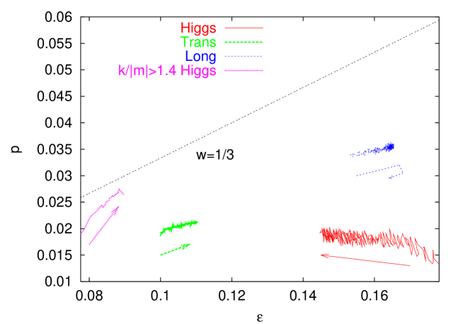
Figure 1: Trajectories of the transversal and longitudinal gauge and the scalar Higgs degrees of freedom in the energy-density - pressure plane (both measured in $|m|^{4}$ units). The longitudinal degree of freedom receives 60-70% more energy from the spinodal instability than the transversal polarisations. The gauge fields display linear equation of state very early. The average slope of the path of the Higgs field is negative. Restricting to the contribution of high $k$ modes the trajectory will have positive slope (cf. left edge of the figure). The arrows show the time direction.

Another aspect of the degeneracy of the longitudinal and transversal gauge degrees of freedom can be observed when studying the so-called spectral equations of state, introduced in our earlier investigation [6]. Using the spatial Fourier transform of the square-root of the pressure and of the energy density distributions one can compute a spectral power for these quantities. Without any need for explicit construction of the quasi-particle coordinates one implicitly assumes that near equilibrium each mode ${\bf k}$ can be described by small amplitude oscillations of some effective field coordinate and its conjugate momentum. The average kinetic and potential energies of a harmonic oscillator are equal. With this assumption one finds:

$$\displaystyle\overline{\epsilon_{\rho}({\bf k})}={\bf k}^{2}\overline{\rho^{2}}+2\overline{V(\rho)},\qquad\overline{p_{\rho}}=\frac{1}{3}{\bf k}^{2}\overline{\rho^{2}},$$

$$\displaystyle\overline{\epsilon_{T}({\bf k})}={\bf k}^{2}\overline{{\bf A}_{T}^{2}}+e^{2}\overline{\rho^{2}{\bf A}_{T}^{2}},\qquad\overline{p_{T}}=\frac{1}{3}{\bf k}^{2}\overline{{\bf A}_{T}^{2}},$$

$$\displaystyle\overline{e^{2}\rho^{2}\epsilon_{L}}={\bf k}^{2}\overline{\Pi_{L}^{2}}+\overline{e^{2}\rho^{2}\Pi_{L}^{2}},\qquad\overline{e^{2}\rho^{2}p_{L}}=\frac{1}{3}{\bf k}^{2}\overline{\Pi_{L}^{2}}.$$ (4)

If the effective squared mass combinations

$$M^{2}_{eff,\rho}\equiv 2\frac{\overline{V(\rho)}}{\overline{\rho^{2}}},\qquad M^{2}_{eff,T}\equiv e^{2}\frac{\overline{\rho^{2}{\bf A}_{T}^{2}}}{\overline{{\bf A}_{T}^{2}}},\qquad M_{eff,L}^{2}\equiv e^{2}\frac{\overline{\rho^{2}\Pi_{L}^{2}}}{\overline{\Pi_{L}^{2}}}$$ (5)

do not vary with $\bf k$ then the following generic behavior can be seen for the spectral equations of state:

$$w_{i}({\bf k})=\frac{\overline{p_{i}({\bf k})}}{\overline{\epsilon_{i}({\bf k})}}=\frac{1}{3}\frac{{\bf k}^{2}}{{\bf k}^{2}+M_{eff,i}^{2}}.$$ (6)

In the twin figures of Fig.2 one can gain impression of how the spectral equation of state develops in time for the different species. The transversal mode displays a behavior which follows (6) almost perfectly extremely early. Its mass can be extracted from the fit very reliably. Although the high $k$ part of the longitudinal energy density stays anomalously large and therefore the corresponding spectral equation of state drops to zero above some $k$ value, in the low $k$ region its degeneracy with the transversal polarisation (signalling the same mass value) is well fulfilled for $|m|t\geq 60$.

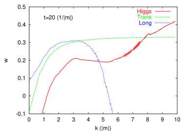
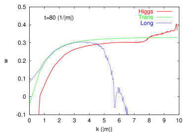
Figure 2: The process of establishing the spectral equation of state for the three particle species. The curves on the left figure are plotted about the time when the linear regime of the global equations of state sets in. Important deviation of the measured curve from (6) is observed for the Higgs field and also for the longitudinal gauge polarisation. The agreement improves substantially at later times (figure on the right). The more persistent deviations in the low $k$ region signal a slow equilibration. ($N=96$, average of 20 independent runs.)

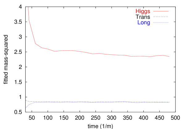
Figure 3: Evolution of the mass-squared values fitted to the spectral EOS with (6). The fitting region was: $0.3<k<5$. The error of the fitted values is approximately 5%. The gauge modes show degeneracy after around $t=60/|m|$.

The onset of the Higgs effect is quantitatively characterised by the degeneracy of the masses fitting the spectral equations of both gauge polarisation states (Fig.3). At the earliest times the longitudinal state is considerably lighter, but we were not able to find an intrinsic Goldstone behavior even at the earliest times when the spectral equation of state already worked.

It is surprising that the spectral equation of state of the Higgs field has qualitatively the expected form in spite the fact that it is far from equilibrium. Its mass value slowly (nearly linearly) relaxes to the non-renormalised (lattice spacing dependent) mass value measured in [6]. This suggests that the mode-by-mode equality of the average kinetic and potential energies is reached very quickly, just the distribution of the power among the different modes is far out of equilibrium.

We conclude this section by discussing some global features of the degree of excitation of the different particle species and their relaxation towards equilibrium. In equilibrium configurations we have shown earlier that the share of the three pieces in the energy density follows the expected 1:1:2 proportion for Higgs, longitudinal gauge and transversal gauge degrees of freedom, respectively.

The main qualitative feature of our simulation is that the longitudinal vector mode is excited during the spinodal instability much more efficiently than the transversal gauge modes. The energy density does not seem to depend qualitatively on whether there are vortices present. The energy exchange on the other hand is much more efficient between the Higgs and the transversal vector modes, than with the longitudinal part. This behavior is very reminiscent of the very slow relaxation of the Goldstone modes in systems which go through the breakdown of a global symmetry [13, 14].

In the case of the vortexed sample an upward deviation can be observed on both the Higgs and the transverse gauge trajectories in the $(p,\epsilon)$ plane towards higher pressures during the annihilation. The sum of the transversal and the Higgs energy densities stays nearly constant during annihilation, while their pressures shoot up. This is intuitively expected since the contribution from the vortex solution to the pressure is negative. The annihilations speed up considerably the energy exchange between these degrees of freedom. The longitudinal modes hardly participate in this process. In an expanding universe one might therefore conjecture that the longitudinally polarised gauge particles never reach thermal equilibrium and when decouple they might store much more energy than one would deduce from calculations based on the assumption of thermal equilibrium.

4 Hausdorff-dimension of the Higgs-defect manifold

In the $U(1)$ Higgs system there are stable topological defects: the Nielsen-Olesen vortices, which are identified as one dimensional defect lines in the Higgs-field. Spontanously emerging long-lived vortex-antivortex configurations, which wind around the whole lattice, thus can be characterized by a stationary non-zero volume fraction of near-zero sites $(\rho<\rho_{th})$ of the Higgs field. The volume fraction grows with the increase of the threshold value $\rho_{th}$.

Vortexed configurations branch-off at a certain time from the uniform exponentially decreasing tendency of the volume fraction of low Higgs values, characteristic for all runs at early times. The branching happens at around $t=50/|m|$. Until this happens, the fraction of the low Higgs values already performed several oscillations. This makes clear that building up of stationary vortex configurations requires considerable time beyond the first appearence of islands of near zero Higgs values after the first roll-down. Not all near zero sites necessarily belong to some vortex. Lower and higher dimensional (possibly) fractal submanifolds will decay and should be left out of consideration when one asks for the early time density of those Higgs-defects which eventually end up in quasilinear, long lived vortex configurations. A sustained non-zero value of the volume fraction of such defects indicates the presence of a (quasi) stationary vortex system until a sudden jump to near-zero values signals the annihilation of the vortex network.

Our final goal is to analyse the variation of the density of the emerging one-dimensional Higgs defect manifold when some characteristic time of the nonequilibrium transition is varied. Earlier investigations [15] were mainly done in two dimensions and identified visually the corresponding topological defects (domain walls). Deviations from the predicted scaling law for the summary length of the domain walls were associated with the contamination arising from random sign-changes of the field, which were abundantly present in the early time evolution of the system. The systematic selection of objects with uniform dimensionality is an unavoidable precondition since any Kibble–Zurek-type analysis makes sense only for objects of well-defined dimensional extension [16, 17]. For the Abelian Higgs model the late(!) time evolution of well developed three-dimensional vortex networks was followed by identifying the vortices through gauge invariant zeros of the Higgs field and also by identifying bits of a vortex through $2\pi$ winding of the $U(1)$ phase [18].

The study of the statistics of the vortex generation requires the identification of Higgs defect lines the earliest possible time after the spinodal instability starts. Here we propose to introduce a ”filtering” step into the identification process of strings: the measurement of the Hausdorff-dimension ($d_{H}$) of the defect manifold consisting of near zero values of the Higgs field. We shall see that it changes during the roll-down of the system and will be able to find systematically the time interval and the range of the coupling parameters where mainly one-dimensional objects are present.

Let us perform a sequence of blocking transformations which leads to the determination of $d_{H}$. One starts by defining the lattice site manifold of the defects for the original Higgs-configuration $\rho_{old}({\bf x})$:

$$X_{old}[\rho_{th}]=\{{\bf x}=(l,m,n)|\rho_{old}(l,m,n)<\rho_{th}\}.$$ (7)

For the formation of the new manifold one considers the blocked lattice with rescaled lattice spacing $pdx$ and site coordinates $(L,M,N)pdx$. The value of the block field is defined as

$$\rho_{new}(L,M,N)=\min\{\rho_{old}(l,m,n)|l=Lp+i,m=Mp+j,n=Np+k,0\leq(i,j,k)<p\}.$$ (8)

The blocked defect manifold is defined as

$$X_{new}[\rho_{th}]=\{{\bf x}=(L,M,N)|\rho_{new}(L,M,N)<\rho_{th}\}.$$ (9)

The number of blocks belonging to $X$ should scale with the dimension of the manifold if it corresponds to objects of well-defined dimensionality embedded in the three-dimensional space:

$$\frac{N(X_{new})}{N(X_{old})}=p^{-d_{H}}.$$ (10)

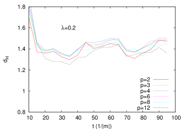
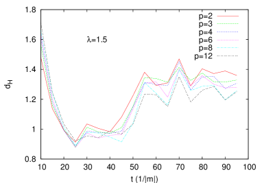
Figure 4: The time evolution of $d_{H}$ calculated from different $p$ values, typical for the distinct $\lambda$ regions (see text).

We have investigated first the time evolution of $d_{H}$ for solutions belonging to the same value of $|m|dx,\rho_{th}$, but different $\lambda$. For each $\lambda$ value $n\geq 10$ independent runs were analysed, starting from different initial conditions. For each run at a given time $|m|t$ blocking transformations with a number of scale factors $p=2,3,4,6,8,12$ were performed and $d_{H}(p)$ was calculated from (10). In Figure 4 we show the time variation of Hausdorff-dimensions calculated with different $p$ for two characteristic values of $\lambda$. In the left hand picture the unique curve, rather independent of the actual value of $p$ proves that the functional form conjectured in (10) is obeyed. However, for such low values ($\lambda<0.5$) the $d_{H}(t)$ function stays well above unity. We checked that in this region no vortices winding around the lattice stabilize for larger times, although the early temporary presence of closed stringlike objects can be observed. Very recently the production of vortices even with higher windings was demonstrated for $\lambda<3e^{2}$ [19]. The difference between the conclusions of the two studies could be twofold: i) our lattices are 8-64 times smaller than those used in [19], and these authors emphasized the need for very large size initial blobs of Higgs defects for vortex formation, ii) the difference between the dynamical processes leading to vortex formation in the two numerical simulations might be important.

We had to exclude this $\lambda$-region ($\lambda<0.5$) from the further analysis, because of the apparent absence of any time interval when the system would be dominated by linear Higgs-defects.

The right hand curves exemplify the behavior of $d_{H}(t)$ estimators from the use of different scale $p$ for the blocking in the range $\lambda>1$ where the unit value of $d_{H}(t)$ is reached at least for a restricted time interval. In the present run the values arising from using different values of $p$ show small dispersion until $|m|t\leq 60$. The ”evaporation” of the one-dimensional objects apparently makes the concept of Hausdorff dimension less apropriate for the Higgs-defect manifold.

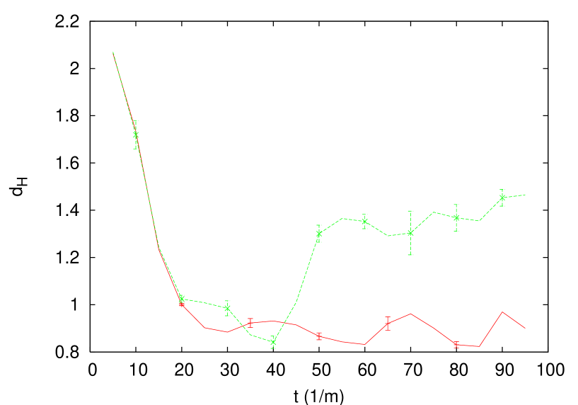
Figure 5: Two typical shapes of the $d_{H}(t)$ function for $\lambda=3,|m|dx=0.35$ and $\rho_{th}/\rho_{0}=0.1$. Each point is an average over $d_{H}(p)$ values obtained with 6 different blocking scales. The statistical error bars correspond to the spread of the $d_{H}$ values calculated with different $p$. They do not depend on time when close to unity. The different shapes for $|m|t\geq 50$ sensitively indicate the presence or absence of stable vortices for large times.

For $\lambda\geq 1$ well-defined $d_{H}(t)$ functions emerge which consist of three portions. The fast initial drop goes over into a nearly constant value varying for different runs between $0.9$ and $1.1$. Then around $|m|t=50$ in some runs the function changes steeply, but continously upwards and approaches $d_{H}(|m|t\geq 100)\approx 1.4$. In other runs its fluctuations are prolongated around the unit value. We checked that for the latter case stable vortices winding around the lattice always appear. In the complementary case no macroscopic vortices get stabilized during the late time evolution, which is intuitively expected on the basis of the badly defined dimensionality of the Higgs zeros in this regime. The two types of $d_{H}(t)$ functions are illustrated by the two curves in Fig.5.

In the allowed range of $\lambda$, $d_{H}$ was determined in all runs in the interval $|m|t\in(20,40)$, where the effective defect dimension was nearly one. We have computed the volume fraction of the defects and their effective dimensionality as an average over this time interval. By this averaging the error bar of this estimate of the Hausdorff dimension was further decreased. The dependence of this time averaged value on the lattice spacing and the value of $\rho_{th}$ was further investigated as described next.

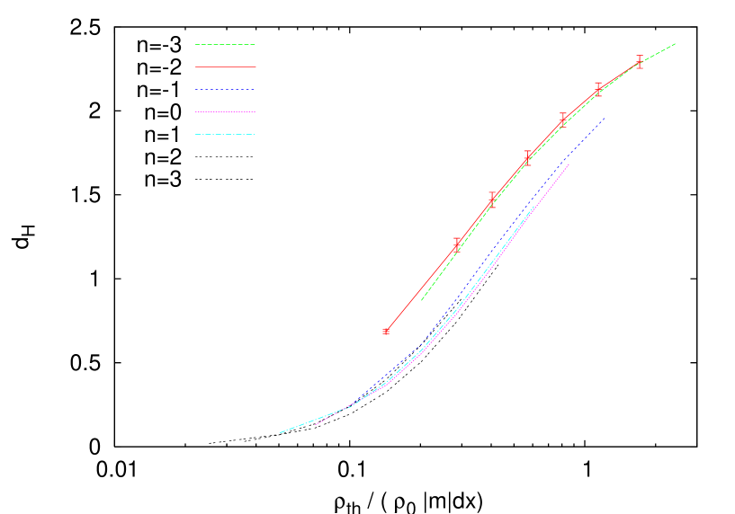
Figure 6: The scaling variation of the Hausdorff dimension with $\rho_{th}$ for different values of $|m|dx$. $d_{H}$ represents the average of the values taken in the region $|m|t\in(20,40)$. The curves obtained with different $|m|dx$ should coincide if $d_{H}$ depends only on the ratio $\rho_{th}/(\rho_{0}|m|dx)$ and $\rho_{th}$ is scaled appropriately. The violation of the scaling for small $|m|dx$ signals nonlinear decrease of the Higgs field near the location of its zero. Typical error is shown on the $n=-2$ curve.

The next step of the analysis was the investigation of the dependence of $d_{H}$ on $|m|dx$, which is the other independent parameter of the discretized equations of motion. A simple argument can be put forward which suggests that (at least for a certain range of $|m|dx$) its change can be compensated by the variation of $\rho_{th}$, which governs the ”detection efficiency” of vortices. In the interior of a vortex near its center one can assume linear variation of the Higgs field with a slope $\sim m_{Higgs}$. The expected value of the Higgs field at the nearest lattice site can be estimated to be $\rho_{0}m_{Higgs}dx$. Since $m_{Higgs}\sim|m|$, therefore when $|m|dx$ changes, the detectability of a vortex is kept on the same level only if the ”detection threshold” $\rho_{th}$ is also varied accordingly:

$$\rho_{th}\sim\rho_{0}|m|dx.$$ (11)

This observation predicts that the two-variable function $d_{H}(\rho_{th}/\rho_{0},|m|dx)$ actually depends only on the ratio of the two. In Fig.6 this scaling of $d_{H}$ is tested. The measurement was performed for dimensionless mass values characterized by the integer $n$: $|m|dx=0.35\times 2^{n/2},n\in(-3,3)$. The basic curve $(n=0)$ represents the variation of $d_{H}$ with $\rho^{(0)}_{th}=0.1$ for $|m|dx=0.35$. It is obvious that the curves drawn with the shifted $\rho_{th}^{(n)}=2^{n/2}\rho_{th}^{(0)},n\in(-1,3)$ values coincide within the accuracy of the determination (cf. the error bars in Fig.6.). However, the shifted curves redrawn for the most negative values of $n$ (e.g. $-2,-3$) do not obey the scaling behavior, probably because the linear approximation with the slope $m_{Higgs}$ is not valid very near to the zero of the Higgs field. The scaling $|m|dx$ dependence greatly simplifies our analysis, since it is sufficient to analyze the dependence of $d_{H}$ on $\lambda$ with a single $|m|dx$ and a conveniently chosen $\rho_{th}$.

It turns out that in the allowed range of $\lambda$ (e.g. $1\leq\lambda$) the effective dimension gets close to unity when using $\rho_{th}=0.1\rho_{0}$. We fixed eventually those parameters ($|m|dx=0.35,\rho_{th}=0.1\rho_{0}$), whose variation is irrelevant for investigating variations of the density of one-dimensional Higgs-defects. It is the investigation of the dependence of the one-dimensional Higgs-defect density on the coupling $\lambda$, which remains our main task.

The final step is to relate the proliferation of the vortexlike defects to some typical time scale which characterizes the underlying non-equilibrium phase transition. The usual Kibble–Zurek analysis [16, 17] assumes the existence of a second order transition and compares the relaxation time of the system to the quenching time, which characterizes the speed of the order parameter variation during the non-equilibrium phase transition. The density of the defects is determined by the correlation length calculated in the moment of the equality of the relaxation and the quenching times, where the system falls out of equilibrium.

In systems of hybrid inflation the coupling of Higgs-fields to the inflaton perfectly realizes this scenario near the critical inflaton amplitude [15]. In our present investigation, however, the system starts by the sudden quench from an initial state far from equilibrium and the sensitivity to the nature of the symmetry breaking (crossover, 1st or 2nd order transition) is not obvious.

We propose to introduce a new type of characteristic time, to be called the roll-down time $\tau_{r}$ as the time needed for the average Higgs-field to reach its first maximum ($\rho_{max}\geq\rho_{0}$):

$$\tau_{r}=\int_{0}^{\rho_{max}}d\bar{\rho}\left(\frac{d\bar{\rho}}{dt}\right)^{-1},\qquad\bar{\rho}(t)=\frac{1}{V}\int d^{3}x\rho({\bf x},t).$$ (12)

The times characteristic for the phase transition and that of the quench are not related in the present case (the latter is actually zero). It is clear that $\tau_{r}$ is much shorter than the time necessary to reach equilibrium. $\tau_{r}$ is in some way related to the spatial correlation length taken at early times by the following argument. Since the spinodal (or “tachyonic”) instability excites modes with wave numbers $k\leq|m|$, therefore directly after its saturation the typical size of homogenous domains is $\xi\sim|m|^{-1}$. The question is, how the roll-down time scales with $|m|$?

We have varied $\lambda$ by keeping the height of the potential $V(0)-V(\rho_{0})=3m^{4}/2\lambda$ fixed. In this way the location of the minimum of the potential was varied $\rho_{0}=(-6m^{2}/\lambda)^{1/2}\sim|m|^{-1}$. Taking into account the fixed height of the potential also $\tau_{r}\sim\lambda^{-1/4}$ is valid. Therefore the smaller is $\lambda$ the longer is the transition time $\tau_{r}$. We have measured its dependence on $\lambda$ through the vacuum expectation values of the Higgs-field:

$$\tau_{r}\sim\rho_{0}^{1/y}\sim|m|^{-1/y},\qquad 1/y=0.64\pm 0.01.$$ (13)

This relation reveals a space-time anisotropy in this sytem, the roll-down time and the spatial correlation length scale differently. It leads to a nontrivial mapping of the $\lambda$-dependence of the defect density into a function of $\tau_{r}$.

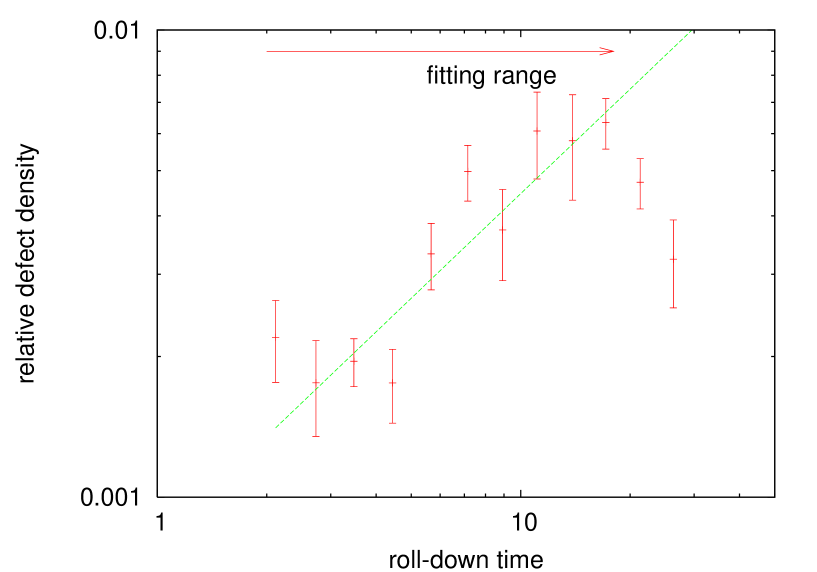
Figure 7: The variation of the volume fraction of the Higgs defects defined at $\rho_{th}=0.1\rho_{0}$ with the roll-down time. On log-log scale Kibble-Zurek scaling implies variation along a straight line.

The defect density was fitted with an exponential decay in the time range: $(20,40)|m|^{-1}$. The fit was then extrapolated back to time $\tau_{r}$ to get the initial defect density $N_{0}$ . The dependence of the initial defect density on $\tau_{r}$ is displayed in Fig.7. In the range displayed on the figure a power law fit was made to it:

$$N_{0}\sim\tau_{r}^{z},\qquad z=0.7\pm 0.4.$$ (14)

The large error is the sum of two effets. The statistical error of the slope determination contributes cca. $0.15$, the rest is the result of some systematics related to the choice of the time interval where the exponential fit is made.

If we are interested in the density of the vortices we have to count only once the Higgs defect sites belonging to the same vortex, that is we have to divide $N_{0}$ by the average length of a vortex, e.g. $\xi$. Therefore we find

$$n_{vortex}\sim\tau_{r}^{z-y},\qquad z-y\approx-0.9\pm 0.4.$$ (15)

This estimate hints at a sharper decrease of the vortex density than proposed in [17], but the large error does not allow to draw a definite conclusion yet whether the vortex density decreases with an exponent different from the case discussed in [10, 11].

5 Conclusions

We have presented a detailed study of the temporal evolution during the non-equilibrium transition leading to the Higgs-effect in classical scalar electrodynamics at sufficiently low energy density. The quick appearance of the degeneracy of longitudinal and transversal gauge excitations is reflected both in the straight line trajectory of these degrees of freedom in the $(p-\epsilon)$-plane, and by the spectral equations of state except the modes with the lowest and the very high wave numbers. This represents a clear evidence for the so-called prethermalisation [20]. On the other hand the degree of excitation of the longitudinal modes is much higher in tachyonic instability, and they relax very slowly. They might decouple during the cosmological expansion with a higher effective temperature than the transversal modes do. Late time decay of the hotter longitudinal modes might produce more energetic charged particles which could participate in elementary processes of cosmological interest.

In this paper also a method was proposed for a refined estimate of the density of stringlike objects present in the whole sample for a certain range of the coupling $\lambda$. The change in the other coupling $|m|dx$ always could be compensated by the resolution parameter $\rho_{th}$. The measurement was performed and averaged in an intermediate time interval ($|m|t\in(20,40)$) and the resulting defect density displays powerlike behaviour as a function of the time characteristic for the transition from the unstable into the stable symmetry breaking minimum. The accuracy of the determination of its power at present is rather poor. Our result indicates that the Kibble–Zurek-scaling phenomenon (not neceesarily with a universal scaling power) may not be tied to the existence of an equilibrium second order transition in the system.

References

- [1] A.D. Linde, Hybrid inflation Phys. Rev. D49 (1994) 748 [astro-ph/93070002]
- [2] G.N. Felder, J. Garcia-Bellido, P.B. Greene, L. Kofman, A.D. Linde and I. Tkachev, Phys. Rev. Lett. 87 (2001) 011601
- [3] T. Asaka, W. Buchmüller and L. Covi, Phys. Lett. B510 (2001) 271
- [4] for the latest developments, see the review of J. Smit in Procs. of SEWM’04, World Scientific 2005, eds. K.J. Eskola, K. Kainulainen, K. Kajantie and K. Rummukainen, pp. 137-146
- [5] J.-I. Skullerud, J. Smit and A. Tranberg, JHEP 08:045, 2003
- [6] D. Sexty and A. Patkós, Phys. Rev. D71:025020 (2005)
- [7] D. Podolsky, G.N. Felder, L. Kofman and M. Peloso, hep-ph/0507096
- [8] M. Hindmarsh and A. Rajantie, Phys. Rev. Lett. 85, 4660 (2000)
- [9] M. Hindmarsh and A. Rajantie, Phys. Rev. D64:065016 (2001)
- [10] T.W.B. Kibble, J. Phys. A9 (1976) 1387
- [11] W.H. Zurek, Nature 317 (1985) 505
- [12] J. Smit, V.C. Vink and M. Sallé, hep-ph/0112057, Presented at COSMO-01, Rovaniemi, Finland 2001
- [13] R. Pisarski and M. Tytgat, Phys. Rev. D54 (1996) 2989
- [14] Sz. Borsányi, A. Patkós and D. Sexty, Phys. Rev. D66:025014 (2002)
- [15] E.J. Copeland, S. Pascoli and A. Rajantie, Phys. Rev. D65:103517 (2002)
- [16] P. Laguna and W.H. Zurek, Phys. Rev. Lett. 78 (1997) 2519
- [17] P. Laguna and W.H. Zurek, Phys. Rev. D58 (1998) 085021
- [18] G. Vincent, N.D. Antunes and M. Hindmarsh, Phys. Rev. Lett. 80 (1998) 2277
- [19] M. Donaire and A. Rajantie, hep-ph/0508272
- [20] J. Berges, Sz. Borsányi and C. Wetterich, Phys. Rev. Lett. 93:142002 (2004)