BNL-HET-05/10, CU-TP-1127, KANAZAWA-04-13, RBRC-486 The Kaon $B$-parameter from Quenched Domain-Wall QCD

Abstract

We present numerical results for the kaon $B$-parameter, $B_{K}$, determined in the quenched approximation of lattice QCD. Our simulations are performed using domain-wall fermions and the renormalization group improved, DBW2 gauge action which combine to give quarks with good chiral symmetry at finite lattice spacing. Operators are renormalized non-perturbatively using the RI/MOM scheme. We study scaling by performing the simulation on two different lattices with $a^{-1}=1.982(30)$ and 2.914(54) GeV. We combine this quenched scaling study with an earlier calculation of $B_{K}$ using two flavors of dynamical, domain-wall quarks at a single lattice spacing to obtain $B_{K}^{\overline{\rm MS}\ {\rm NDR}}(\mu\!=\!2\,{\rm GeV})=0.563(21)(39)(30)$, were the first error is statistical, the second systematic (without quenching errors) and the third estimates the error due to quenching.

I INTRODUCTION

Kaon decays to two pions provided the first experimental observation of $CP$ violation about four decades ago. This type of $CP$ violation, called indirect $CP$ violation, proceeds via mixing of $K^{0}$ and $\overline{K}^{0}$. Direct $CP$ violation in kaon decays, occurring in the decay process itself, has been accurately measured experimentally relatively recently. Additionally, $CP$ violation has now been observed in the $b$ quark system. The standard model origin of $CP$ violation is the Cabibbo-Kobayashi-Maskawa (CKM) matrix and determining the four real parameters that define this matrix, and looking for physical processes that are not correctly represented by it, is a major focus of particle physics theory and experiment.

In determinations of the parameters of the CKM matrix, the experimental measurements of indirect (represented by the parameter $\epsilon$) and direct (represented by the parameter ${\rm Re}(\epsilon^{\prime}/\epsilon)$) $CP$ violation in kaons should provide important constraints, but relating the experimental values to standard model parameters requires controlled theoretical calculations. These calculations involve using the operator product expansion to separate the problem into its short-distance, and hence perturbatively calculable, components and its long-distance, non-perturbative parts. The short-distance effects in these processes are given by the Wilson coefficients of the operator product expansion Buchalla:1995vs and the matrix elements of the relevant operators in the expansion determine the long-distance parts.

In particular, for indirect $CP$ violation, the hadronic matrix element needed for a theoretical prediction of $K^{0}$–$\overline{K}^{0}$ mixing in the standard model is generally parameterized by the parameter $B_{K}(\mu)$, defined by

$$B_{K}(\mu)\equiv\frac{\langle\overline{K}^{0}|Q^{(\Delta S=2)}(\mu)|K^{0}\rangle}{\frac{8}{3}f_{K}^{2}m_{K}^{2}}\,.$$ (1)

The four-fermion operator appearing in this expression is given by $Q^{(\Delta S=2)}=(\bar{s}\,\gamma_{\nu}(1-\gamma_{5})\,d)\,(\bar{s}\,\gamma^{\nu}(1-\gamma_{5})\,d)$ and the scale dependence, $\mu$, enters when this operator is renormalized. (Here and elsewhere in this paper we will be omitting color indices for simplicity.) If one approximates the numerator in the definition of $B_{K}$ by inserting the vacuum state to achieve two matrix elements of two-quark operators, one gets the value in the denominator. (This is known as the vacuum saturation approximation.) Since this should be a reasonable coarse approximation for the $Q^{(\Delta S=2)}$ matrix element, $B_{K}$ is naturally a quantity of $O(1)$.

Because $B_{K}$ involves physics at low energy scales where non-perturbative QCD effects dominate, numerical simulations of lattice QCD provide the only known first principles method for its calculation. For recent reviews see Refs. Kuramashi:1999gt ; Lellouch:2000bm ; Martinelli:2001yn ; Ishizuka:2002nm ; Becirevic:2004fw ; Wingate:2004xa . Consequently, calculations of $B_{K}$ have been a focus of lattice QCD simulations for two decades. Though achieving an accurate value for this quantity for dynamical fermion simulations is an important goal, a large portion of the calculations done to date are in the quenched approximation. Early calculations used Wilson fermions, which break chiral symmetry, or staggered fermions, which retain a $U(1)$ subgroup of the continuum non-singlet chiral symmetry but break the flavor symmetry of continuum QCD. For Wilson fermions the operator $Q^{(\Delta S=2)}$ can mix with four other lattice operators, with different chiralities, at $O(a^{0})$, making precise calculations difficult ($a$ is the lattice spacing)  Aoki:1999gw ; Lellouch:1998sg . For staggered fermions, many calculations have been done, but the large $O(a^{2})$ scaling violations of this formulation introduce errors in the extrapolation to the continuum limit Aoki:1997nr . Recently, calculations with twisted mass Wilson fermions Dimopoulos:2003kc and improved staggered fermions Davies:2003ik ; Aubin:2004wf have been undertaken to reduce these errors.

An important improvement in the lattice techniques for calculating $B_{K}$ (and other hadronic matrix elements) has been the development of fermion formulations which preserve the chiral symmetries of QCD arbitrarily well at finite lattice spacing Neuberger:1997fp . Two common versions of these formulations are domain-wall fermions  Kaplan:1992bt ; Shamir:1993zy ; Furman:1995ky , which we will use here, and overlap fermions Neuberger:1998my ; Edwards:1998yw . For domain-wall fermions with their controllable breaking of the continuum $SU(N_{f})_{L}\otimes SU(N_{f})_{R}$ symmetry group at finite lattice spacing, mixing of lattice operators, including mixing with chirally disallowed operators, is under control and non-perturbative renormalization techniques have been shown to work well for the relation of lattice operators to continuum operators Blum:2001sr ; Blum:2001xb . Also, controlling chiral symmetry at finite lattice spacing removes the $O(a)$ scaling violations, reducing deviations from the continuum limit for domain-wall fermions at finite values of $a$.

In this paper, we present our quenched calculation of $B_{K}$ and basic low-energy hadronic quantities using the domain-wall fermion action and the DBW2 (Doubly Blocked Wilson in two-dimensional parameter space) gauge action Takaishi:1996xj ; deForcrand:1999bi . Domain-wall fermions introduce a fifth dimension of length $L_{s}$, with a coordinate $s$ ( $0\leq s\leq L_{s}-1$) in which the gauge fields are simply replicated, and produce light, left-handed quark states bound to the four-dimensional boundary hypersurface (domain-wall) with $s=0$ and right-handed quark states on the boundary with $s=L_{s}-1$. Four-dimensional quark fields are constructed from the chiral modes on the boundaries, with the residual chiral symmetry breaking controlled by the size of $L_{s}$. Previous works  Blum:1997jf ; Blum:1997mz ; AliKhan:2000iv ; Blum:2000kn have extensively studied the behavior of domain-wall fermions in quenched QCD, in particular the dependence of the residual chiral symmetry breaking effects on $L_{s}$. The CP-PACS Collaboration AliKhan:2000iv reported that the residual chiral symmetry breaking for domain-wall fermions in quenched QCD is markedly reduced by the use of a renormalization group improved gauge action (Iwasaki gauge action), which was also studied by the Columbia group and the smaller chiral symmetry breaking was found to not persist for dynamical simulations Mawhinney:2000fw . Subsequently, the RBC Collaboration  Aoki:2002vt found the further suppression of the chiral symmetry breaking by using the DBW2 gauge action, which was originally introduced as an approximation to the renormalization group flow for lattices with $a^{-1}\approx 2$ GeV Takaishi:1996xj ; deForcrand:1999bi . As discussed later in this paper, the Iwasaki and DBW2 actions are closely related, differing only in the choice of a single parameter.

Compared to the $a\to 0$ value of $0.628(42)$ found by the JLQCD collaboration using naive staggered fermions Aoki:1997nr , previous quenched calculations of $B_{K}$ with domain-wall fermions have given a lower value. The CP-PACS collaboration, using the Iwasaki gauge action and perturbative renormalization, measured $B_{K}$ for two lattice spacings and different volumes and quoted a value of $0.5746(61)(191)$ for $a\to 0$  AliKhan:2001wr . The RBC collaboration reported a value of $0.532(11)$ using the Wilson gauge action and a single lattice spacing of $a^{-1}=1.92(4)$ GeV Blum:2001xb and a value of 0.495(18) in a full QCD simulation with the DBW2 gauge action and two-flavors of dynamical quarks at a lattice spacing of $a^{-1}=1.691$ GeV Aoki:2004ht . All of the values quote above refer to the $B_{K}$ defined in the $\overline{\rm MS}$ scheme using naive dimensional regularization and a renormalization scale $\mu=2.0$ GeV. This quantity has also been measured in quenched QCD using the closely related overlap formulations Garron:2003cb ; DeGrand:2003in . Here we report on calculations at two lattice spacings, $a^{-1}=1.982(30)$ and $2.914(54)$ GeV, allowing the determination of the $a\to 0$ value for $B_{K}$. In addition, we compare with the previous RBC two-flavor result to estimate the error introduced by the quenched approximation. The smaller residual chiral symmetry breaking for the DBW2 gauge action allows us to check whether physical results depend on this residual breaking.

The remainder of this paper is organized as follows. Section II is devoted to a description of the details of our numerical simulations and the issues of generating an ensemble of configurations with the DBW2 gauge action which sample different topological sectors. Our results for basic quantities such as the hadron spectrum and the residual chiral symmetry breaking are presented in Section III. We present the details of the calculation of the decay constants of the pseudoscalar meson in Section IV. One of the features of our calculation is the use of non-perturbative renormalization (NPR) in the determination of the renormalization factors needed to relate the lattice operators to their continuum counterparts. We deal with this topic in Section V. In Section VI, we construct physical results for $B_{K}$, compare our result with previous work and discuss the potential systematic errors for our result. Section VII gives our conclusions. Preliminary results of the calculations presented here have been given in Refs. Noaki:2002ai ; Noaki:2003vr .

II DETAILS OF NUMERICAL SIMULATIONS

II.1 Simulation Parameters

The main results of this paper are from two ensembles of quenched configurations, one with $a^{-1}=1.982(30)$ GeV and the second with 2.914(54) GeV, which are generated with the DBW2 gauge action with $\beta=1.04$ and 1.22, respectively. The DBW2 action is defined by

$$S_{G}[U]=-\frac{\beta}{3}\left[(1-8\,c_{1})\sum_{x;\mu<\nu}P[U]_{x,\mu\nu}+c_{1}\sum_{x;\mu\neq\nu}R[U]_{x,\mu\nu}\right]$$ (2)

where $P[U]_{x,\mu\nu}$ and $R[U]_{x,\mu\nu}$ represent the real part of the trace of the path ordered product of links around the $1\times 1$ plaquette and $1\times 2$ rectangle, respectively, in the $\mu,\nu$ plane at the point $x$ and $\beta\equiv 6/g^{2}$ with $g$ the bare coupling constant. For the DBW2 gauge action, the coefficient $c_{1}$ is chosen to be $-1.4069$, using the criteria that this action is a good approximation to the renormalization group flow for lattices with $a^{-1}\simeq 2$ GeV  Takaishi:1996xj ; deForcrand:1999bi . The DBW2 action is a particular choice of the class of improved actions given by plaquette and rectangle terms, with the Iwasaki action Iwasaki:1983ck ; Iwasaki:1985we being another common choice. However, as was demonstrated in Ref. Aoki:2002vt , the DBW2 action produces smaller residual chiral symmetry breaking, at a given lattice spacing and $L_{s}$, than the Iwasaki action. Our conventions for the domain wall fermion operator are as in Ref. Blum:2000kn .

We will also have reason to compare our DBW2 results to those obtained on quenched configurations generated with the Wilson gauge action, with $a^{-1}=1.922(43)$ GeV. These configurations were analyzed in detail in Refs. Blum:2000kn ; Blum:2001xb . Table 1 lists simulation parameters for the numerical calculations we present in this paper. In this table and following in this paper, we refer our ensembles as “DBW2 $\beta=1.22$”, “DBW2 $\beta=1.04$”and “Wilson $\beta=6.0$”. The number of configurations used for each quantity are given, with those in bold denoting new calculations for this work. For the quantities where the number of configurations is followed by an asterisk, we employed wall-source quark propagators which were an average of quark propagators with periodic and anti-periodic boundary conditions in the time direction. These doubled the period of the correlation functions and removed contributions to our correlation functions from states propagating backward through the time boundaries of our lattices. The quark masses $m_{f}$ used for each calculation are listed in Table 2.

II.2 Configuration Generation with the DBW2 Action

As mentioned previously, we have used the DBW2 gauge action for this work, since our earlier studies Aoki:2002vt showed this action produced a pronounced decrease in the residual chiral symmetry breaking for domain-wall fermions. This decrease occurs because the DBW2 action gives rise to smoother gauge fields at the scale of the lattice spacing, when compared to other actions at the same lattice spacing. This smoothness means smaller perturbative contributions to the residual chiral symmetry breaking as well as many fewer lattice dislocations, where by dislocation we mean a localized change in the topology of the gauge field which produces eigenmodes of the domain-wall fermion operator which are undamped in the fifth dimension. It should be emphasized that the DBW2 action does not suppress large, physical topological objects, but merely small dislocations where topology is changing. This desired suppression of lattice dislocations has the unwanted effect of causing current heat-bath and overrelaxed pure gauge algorithms to sample different topological sectors quite slowly.

Since topological charge changes less frequently with the DBW2 gauge action than other choices for the gauge action, one should check the distribution of the topological charge for an ensemble under study. In Ref. Aoki:2002vt , topology change for one of our choices of parameters, DBW2 with $\beta=1.04$ was examined. By using many steps of a combined heat bath and overrelaxed algorithm, a practically acceptable frequency for topology change was observed. However, here we are also interested in DBW2 lattices with $\beta=1.22$. At this much weaker coupling and smaller lattice spacing, the time for topology change with known algorithms should be much longer. (We will say more about this time scale shortly.) We were forced to consider how to generate a distribution of DBW2 lattices at this lattice spacing, including configurations of different topology. The different topological sectors for DBW2 should be distinguished by large, physical topological objects.

Consider the partition function for quenched QCD in a particular topological sector with topology $n$. For the DBW2 action, this is explicitly given by

$$Z^{(n)}_{\rm DBW2}=\int_{n}[dU]e^{-S_{\rm DBW2}}$$ (3)

where only gauge fields with topology $n$ enter. Of course this requires a precise definition of the topology of the gauge field and one could use the domain-wall fermion operator, for arbitrarily large $L_{s}$, to determine this. With the assumption that current algorithms do not change the topology for DBW2 lattices with $\beta=1.22$, a thermalized lattice with topology $n$ will remain in this topological sector. This makes it straightforward to measure the expectation value $\langle{\cal O}\rangle_{n}$ of an observable $\cal O$ in the topological sector $n$ from a starting lattice with a given topology. Since $Z=\sum_{n}Z_{\rm DBW2}^{(n)}$, we have

$$\langle{\cal O}\rangle=\frac{\sum_{n}Z_{\rm DBW2}^{(n)}\langle{\cal O}\rangle_{n}}{\sum_{m}Z_{\rm DBW2}^{(m)}}$$ (4)

and we require the ratio $Z^{(n)}_{\rm DBW2}/Z^{(m)}_{\rm DBW2}$, for configurations in topological sectors $n$ and $m$, to determine $\langle{\cal O}\rangle$. Unfortunately, this ratio is not simple to determine.

We can, however, approximate this ratio using a corresponding ratio with the standard Wilson gauge action at the same lattice spacing and volume, i.e.

$$\frac{Z^{(n)}_{\rm DBW2}}{Z^{(m)}_{\rm DBW2}}\approx\frac{Z^{(\bar{n})}_{\rm Wilson}}{Z^{(\bar{m})}_{\rm Wilson}}$$ (5)

where the $\bar{n}$ and $\bar{m}$ variables denote that topology in the Wilson case is determined only from the long-distance features of the gauge fields, $n=\bar{n}$ and $m=\bar{m}$. This approximation is motivated by the expectation that large-scale, physical topological fluctuations will be the same for any two theories that differ only in their cut-off behavior at short distances. This is a standard statement of field theory. An alternative way of expressing this is to consider the topological susceptibility. When averaged over all topological sectors, it should give the same result for Wilson and DBW2 actions at weak coupling, provided the susceptibility is renormalized correctly in both cases. Renormalization improvement removes the dependence on the ultraviolet parts of the theory and is equivalent to using only large-scale topological objects in determining $\bar{n}$ and $\bar{m}$.

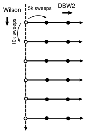
Figure 1: A schematic of our algorithm for generating gauge configurations with the DBW2 action and $\beta=1.22$. We first produce gauge configurations using the Wilson gauge action with $\beta=6.25$ (vertical direction) and save them every 10,000 sweeps (open circles). These saved configurations are used as the initial configuration for a subsequent DBW2 evolution with $\beta=1.22$ (horizontal direction).

To use Eq. 5 to generate an ensemble of DBW2 configurations with the correct large-scale topological fluctuations of quenched QCD for DBW2 with $\beta=1.22$, we proceed as sketched in Fig. 1. We first generate gauge configurations using the standard Wilson gauge action with $\beta=6.25$, denoted by proceeding down the vertical dashed line in Fig. 1. By using $m_{\rho}=770$ MeV as input, these lattices have a lattice spacing of $2.808(49)$ GeV with $L_{s}=8$ and $M_{5}=1.7$ for 50 configurations. Alternatively we can use the heavy quark potential to set the scale. With the parameterization in Ref. Guagnelli:1998ud and a value for the Sommer scale, $r_{0}$, of 0.5 fm, we obtain $a^{-1}=3.12$ GeV for the lattices with Wilson gauge action, which is close to the lattice spacing of $a^{-1}$ = 3.09(2) GeV as determined by the heavy quark potential for $\beta=1.22$ Hashimoto:2004rs . Every 10,000 heatbath sweeps (the white circles in Fig. 1), a Wilson lattice is saved to use as a starting point for a DBW2 evolution (the horizontal lines in Fig. 1). Assuming the initial Wilson gauge configurations effectively sample the different topological sectors, we are then beginning each DBW2 evolution from a starting configuration which reflects the appropriate large-scale topological distribution of quenched QCD. The parameters of the DBW2 evolution are chosen to yield the same lattice spacing as in the Wilson evolution. We evolve using DBW2 to reach an equilibrated ensemble for DBW2, but in a particular topological sector, assuming that the topology does not change during the DBW2 evolutions. We can then average observables from the different DBW2 evolutions together, since the probability of each topology appearing is controlled by the Wilson action and Eq. 5 relates the Wilson and DBW2 quantities.

For observables that are not sensitive to short-distance topological features, the algorithm above should provide a good approximation to a full DBW2 ensemble average. The appropriately renormalized topological susceptibility is an example. However, an uncontrolled approximation in this algorithm is how the topology in the initial Wilson action changes as the DBW2 evolution thermalizes. Small size topological defects in the Wilson lattice are suppressed by the DBW2 action. Defects which are removed, leaving the topology unchanged, cause no uncertainty. Defects which are removed by becoming larger in size can contribute to the topology as determined on large distance scales and make a topology in the DBW2 case appear with an incorrect probability.

Overall, we used 53 initial Wilson configurations (the open circles in Fig. 1) and 53 subsequent independent DBW2 evolutions. To check the distribution of topological charge $Q_{\rm top}$ for our ensembles, we have calculated it for configurations indicated by the open and filled circles in Fig. 1, a la the MILC Collaboration DeGrand:1997ss ; Aoki:2004ht . Figure 2 shows the result in the form of a time history and distribution of the topological charge for three ensembles of 53 lattices: one with no DBW2 sweeps (the initial 53 Wilson configurations); the second generated from the initial Wilson configurations with 5,000 DBW2 over-relaxed/heatbath sweeps; the third generated with 10,000 DBW2 sweeps. These appear in Fig. 2 from the top to bottom panels, respectively. It is apparent from the figure that the topology, as measured using the smearing technique of Ref. DeGrand:1997ss , changes little during a DBW2 evolution. During the 10,000 sweeps done for these 53 different evolutions, 21 evolutions changed topology once and the others did not. Of the 21 evolutions which changed topology, 19 changed in the first 5,000 sweeps. Averaging over each ensemble, we obtain $\left\langle Q_{\rm top}\right\rangle=0.18(43)$ (0 sweeps), $0.36(40)$ (5,000 sweeps) and $0.40(40)$ (10,000 sweeps). Taking the last two ensembles together, our DBW2 ensemble has $\left\langle Q_{\rm top}\right\rangle=0.38(29)$.

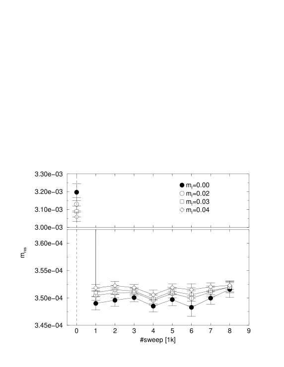
Figure 3: $m_{\rm res}$ as a function of the number of sweeps for the DBW2 evolutions with $\beta=1.22$. $m_{\rm res}$ was measured for $L_{s}=8$ and $M_{5}=1.7$ and these results are averaged over 20 of the 53 DBW2 evolutions.

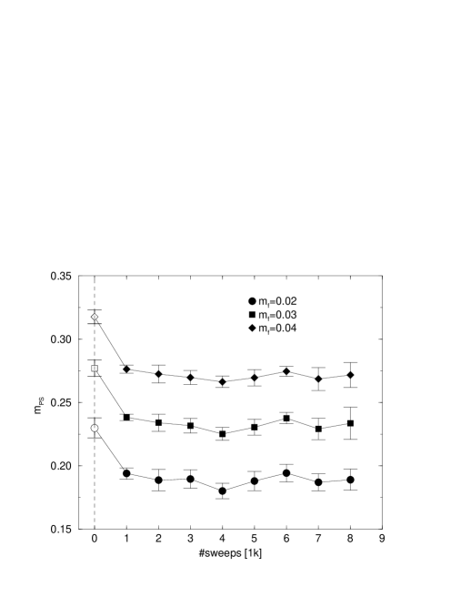
Figure 4: The pseudoscalar meson mass, $m_{\rm PS}$, as a function of the number of sweeps in the DBW2 evolution.

For the physical observables reported in this paper (the DBW2 $\beta=1.22$ column of Table 1), we collected one or two configurations from either 5,000 or 10,000 sweeps in each of the 53 DBW2 evolutions. To check for thermalization effects in the DBW2 evolutions, we measured the residual quark mass, whose definition is given in Eq. 8, and pseudoscalar meson mass, $m_{\rm PS}$, after every 1,000 over-relaxed/heatbath sweeps with $L_{s}=8$ and $M_{5}=1.7$. The results for $m_{\rm res}$ from the first 20 configurations in the direction of the Wilson sweep are shown in Fig. 3 for different values of the quark mass, $m_{f}=0.02,\ 0.03$ and $0.04$ (open symbols) and those in the chiral limit from the linear fit (filled symbols). The vertical axis is divided into two parts, since the residual mass for the initial (Wilson) lattices is about an order of magnitude greater than for the DBW2 lattices. No thermalization effects are visible after the first 1,000 sweeps, but clearly the result for $m_{\rm res}$ shows that lattice dislocations have been markedly reduced. Figure 4 shows the same kind of plot for $m_{\rm PS}$. Again, no thermalization effects are visible here, after the first 1,000 sweeps. From this we see that DBW2 lattices separated by 5,000 sweeps are thermalized.

We thus conclude that we have generated a thermalized distribution of DBW2 lattices, with a distribution of large-scale topological features that is a good approximation to the exact distribution. Our strategy is based on the assumption that a modification of the ultraviolet properties of the theory, such as the RG-improvement of the action, does not change the infrared properties of the theory, such as topology. The measurements discussed here show that the approximation is working quite well. We believe this approach to be superior to either working in a single topological sector, since our lattice volumes are not large, or averaging randomly over topologies, since that ignores the underlying QCD dynamics. Of course, having a pure-gauge updating algorithm which rapidly samples different topological sectors at weak coupling would be a better solution, but with this current approach we now turn to the measured meson masses.

III VECTOR AND PSEUDOSCALAR MESON MASSES

In this section we discuss the calculation of meson masses and use them to determine values for the basic parameters of the simulation, such as the residual quark mass, $m_{\rm res}$, the lattice spacing, $a$, and the bare quark mass which produces a pseudoscalar meson with the physical kaon mass when made from two degenerate quarks.

We have measured the wall-point and wall-wall two-point correlation functions

$${\cal C}_{\rm pw}^{\Gamma_{1}\Gamma_{2}}(t,t_{0}) = \left\langle 0\left|\phi_{\Gamma_{1}}(t)\,\chi_{\Gamma_{2}}^{\dagger}(t_{0})\right|0\right\rangle,$$ (6)

$${\cal C}_{\rm ww}^{\Gamma_{1}\Gamma_{2}}(t,t_{0}) = \left\langle 0\left|{\chi_{\Gamma_{1}}(t)\,\chi_{\Gamma_{2}}^{\dagger}(t_{0})}\right|0\right\rangle,$$ (7)

where $\phi_{\Gamma}(t)$ and $\chi_{\Gamma}(t)$ are quark bilinear interpolating fields with the Dirac spinor structure $\Gamma=V_{\mu},A_{\mu},S$ and $P$. The quantity $\phi_{\Gamma}(t)$ is a local, bilinear field, summed over a spatial volume at fixed time $t$, that is $\phi_{\Gamma}(t)=\sum_{\bf x}\bar{q}({\bf x},t)\,\Gamma\,q({\bf x},t)$. In contrast, $\chi_{\Gamma}(t)$ is a spatially non-local bilinear defined on a three-dimensional volume at fixed time. In particular, $\chi_{\Gamma}(t)=\sum_{{\bf x},{\bf y}}\bar{q}({\bf x},t)\,\Gamma\,q({\bf y},t)$ for Coulomb gauge fixed quark fields $q$ on time-slice $t$.

As explained in Section II.1, we first compute quark propagators with both periodic and anti-periodic boundary conditions in the time direction in evaluating the correlation functions in Eqs.  6 and 7 from certain ensembles. To extract the masses and amplitudes for states entering these correlation functions, they are fit to the hyperbolic functions ${\cal A}\sinh(m(t-t_{0}-T/2))$ or ${\cal A}\cosh(m(t-t_{0}-T/2))$, depending on the symmetry of the interpolating fields being used. Here ${\cal A}$ and $m$ are fitting parameters and $T$ is twice the time extent of the lattice, due to our choice of quark propagators. We note that in our earlier quenched work Blum:2000kn ; Aoki:2002vt for the Wilson $\beta=6.0$ and DBW2 $\beta=1.04$ actions, we did not calculate two-point correlation functions on doubled lattices. A further improvement in the present work is the use of two-point correlators which are the average of two point functions obtained from each of the two sources that were introduced to compute the three point functions. The data obtained in this way are marked with *’s in Table 1.

For domain-wall fermion simulations the finite extent of the fifth dimension produces chiral symmetry breaking effects in the low-energy QCD physics represented by the domain-wall fermion modes localized on the boundaries of the fifth dimension. We first turn to a determination of this residual chiral symmetry breaking since it is of both intrinsic interest and is needed for all extrapolations to the zero (renormalized) quark mass limit. As has been discussed extensively in Ref. Blum:2000kn , for low-energy QCD the residual chiral symmetry breaking will appear as a small additive quark mass, denoted by $m_{\rm res}$, that represents this symmetry breaking in an effective-field theory formulation of QCD.

We calculate $m_{\rm res}$ from the ratio of correlators

$$m_{\rm res}=\left.\frac{\sum_{{\bf x}}\left\langle 0\left|J_{5q}({\bf x},t)\xi_{P}^{\dagger}(0)\right|0\right\rangle}{\left\langle 0\left|\phi_{P}(t)\xi_{P}^{\dagger}(0)\right|0\right\rangle}\right|_{t\gg a},$$ (8)

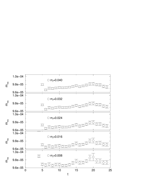
Figure 5: Ratio of the right-hand side of Eq. 8 for the DBW2 $\beta=1.22$ data as a function of $t$. From bottom to top panel, data are plotted in order of lightness of the quark.

where $\xi=\phi$ for Wilson $\beta=6.0$ and DBW2 $\beta=1.04$ and $\xi=\chi$ for DBW2 $\beta=1.22$ depending on an unessential convenience in our numerical simulation. $J_{5q}$ is a pseudoscalar density located at the mid-point of the fifth dimension Furman:1995ky ; Blum:2000kn . In Fig. 5 we show the ratio on the right-hand side of Eq. 8 as a function of $t$ for DBW2 $\beta=1.22$. From the bottom to top, the panels in Fig. 5 show data in order from the lightest $m_{f}$ to heaviest. In choosing the lower bound of the fitting range $t_{\rm min}$, we only need a time separation large enough to remove any contribution from the unphysical, off-shell, five-dimensional states in the DWF theory. We do not need to suppress legitimate excited states of QCD whose contributions will also obey Eq. 8. As suggested by the figure, we could chose $t_{\rm min}$ as small as 4-5 lattice units. For somewhat arbitrary reasons we used the value $t_{\rm min}=14$ which has the effect of somewhat increasing the resulting error on $m_{\rm res}$.

Since the finite $L_{s}$ effects represented by $m_{\rm res}$ arise from short distances, $m_{\rm res}$ should depend only weakly on the quark mass $m_{f}$ and is usually evaluated in the limit $m_{f}\to 0$. A plot of the values of $m_{\rm res}$ as a function of $m_{f}$ is shown in Fig. 6. Included in the figure is a linear fit to the data, which we extrapolate to $m_{f}=0$ to find $m_{\rm res}=0.9722(27)\times 10^{-4}$. The extrapolation changes the value of $m_{\rm res}$ by less than 1%. The coefficients of the linear fit are given in the first row of Table 3. The second and third rows give results for $m_{\rm res}$ previously calculated for other ensembles that will be used in this paper. We note that $m_{\rm res}$ for the Wilson gauge action with $\beta=6.0$ was obtained from simulations with a single quark mass of $m_{f}=0.02$.

In a previous paper on simulations with domain-wall fermions  Blum:2000kn , we included an extensive investigation of the infrared pathologies that occur in the $m_{f}\to 0$ limit of quenched domain-wall fermions, or any other fermionic formulation that preserves the continuum global symmetries of QCD. In this paper, the focus is primarily on physics at the kaon scale, but we will briefly check that our earlier observations are consistent with the data at this weaker coupling. To this end, we now detail our methods for determining physical values from pseudoscalar correlators.

In extracting the low-lying masses and amplitudes from the correlators ${\cal C}_{\rm pw}^{PP}(t,t_{0})$ and ${\cal C}_{\rm pp}^{PP}(t,t_{0})$ it is important to minimize the effects of topological near-zero modes. We described a number of ways to approach this in Ref. Blum:2000kn and noted that the effects of topological near-zero modes decrease as the source-sink separation is made larger. Here we couple this observation with our measurement of correlators on doubled lattices to minimize the effects of topological near-zero modes by choosing a relatively large value of $t_{\rm min}$ when extracting masses and amplitudes.

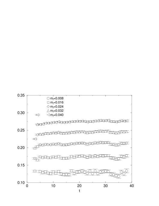
Figure 7: The pseudoscalar effective mass for the DBW2, $\beta=1.22$ data set plotted as a function of the time $t$. This was obtained from the point-wall correlator ${\cal C}^{A_{4}P}_{\rm pw}$.

We now describe our results for the pseudoscalar masses and leave the detailed discussion of the pseudoscalar decay constants to the next section. In Fig. 7 we show the effective mass of the pseudoscalar meson mass as a function of time for the DBW2 $\beta=1.22$ data set obtained from the point-wall correlator ${\cal C}^{A_{4}P}_{\rm pw}$. A fine plateau showing no apparent excited state contamination extends from $t=10$ to $t=38$. Note the source is located at $t=0$ and the symmetric mid-point of our time-doubled lattice is $t=47.5$. In this paper we use an analytic formula to determine the effective mass, $m_{\rm eff}$, from three time separations:

$$m_{\rm eff}=\ln(r(t)+\sqrt{r(t)^{2}-1})$$ (9)

where the ratio $r(t)$ is given by:

$$r(t)=\frac{C(t+1)+C(t-1)}{2\,C(t)}$$ (10)

and C(t) represents one of the two-point correlators defined in Eqs. 6 and 7.

Since the decay constants will be calculated and compared using both ${\cal C}^{A_{4}P}_{\rm pw}$ and ${\cal C}^{PP}_{\rm ww}$ in the following section, we want to compare the amplitudes determined from fitting the two different correlators, while keeping the pseudoscalar mass the same. To achieve this, we extract a common value of $m_{\rm PS}$ from these correlation functions through a simultaneous fit which minimizes the $\chi^{2}$ given by

$$\chi^{2} = \sum_{t=t_{\rm min}}^{t_{\rm max}}\left\{\left[\frac{{\cal C}^{A_{4}P}_{\rm pw}(t,0)-{\cal A}^{A_{4}P}_{\rm pw}\sinh(m_{\rm PS}(t-T/2))}{\sigma^{A_{4}P}_{\rm pw}(t)}\right]^{2}\right.$$ (11)

$$\hskip 28.45274pt+\left.\left[\frac{{\cal C}^{PP}_{\rm ww}(t,0)-{\cal A}^{PP}_{\rm ww}\cosh(m_{\rm PS}(t-T/2))}{\sigma^{PP}_{\rm ww}(t)}\right]^{2}\right\},$$

where $\sigma(t)$ is the jackknife error of the correlator at $t$.

In Ref. Blum:2000kn , it was found that, for Wilson $\beta=6.0$, the zero mode effects seen by comparing scalar and pseudoscalar correlators become small for source-sink separations of 10 lattice spacings. To mitigate these effects in the analysis of this work, we chose the fitting range $(t_{\rm min},t_{\rm max})$ to be $(12,19)$ for DBW2 $\beta=1.04$ and Wilson $\beta=6.0$, both of which correspond to $a^{-1}\approx 2$ GeV. For DBW2 $\beta=1.22$ ($a^{-1}\approx 3$ GeV), we use $(18,31)$ so that $t_{\rm min}=12$ and 18 corresponds to a similar distance in physical units for both lattice spacings. Results for $m_{\rm PS}$ with degenerate and non-degenerate masses for DBW2 $\beta=1.22$ are given in the fourth column of Table 4. Results of the same analysis on the doubled lattice for DBW2 $\beta=1.04$ and Wilson $\beta=6.0$ are listed in the sixth column of Table 5. This table contains previous values for $m_{\rm PS}$ from the point-point correlator ${\cal C}^{PP}_{\rm pp}$ in the fifth column for comparison. The central values agree within the quoted errors, with smaller errors for the results computed on larger ensembles. For the DBW2 action with $\beta=1.22$, we have also calculated $m_{\rm PS}$ from ${\cal C}_{\rm pw}^{A_{4}P}$, ${\cal C}_{\rm pw}^{PP}$ and ${\cal C}_{\rm ww}^{PP}$ separately and the results are consistent with those from the simultaneous fit obtained by minimizing the $\chi^{2}$ given in Eq. 11, within the quoted statistical error.

We now investigate the chiral limit. In Ref. Aoki:2002vt $m_{\rm PS}^{2}$ is fit to the form

$$m_{\rm PS}^{2} = a_{\pi}\,(m_{f}+m_{\rm res})\left[1-\delta\,\ln{\frac{a_{\pi}(m_{f}+m_{\rm res})}{\Lambda_{\chi}^{2}}}\right]+b\,(m_{f}+m_{\rm res})^{2}$$ (12)

with the cutoff $\Lambda_{\chi}=1$ GeV. This expansion includes the pathologies of the quenched approximation $\delta m_{f}\ln{m_{f}}$ making it more difficult to extrapolate to the chiral limit whereas only weaker $m_{f}^{2}\ln{m_{f}}$ terms appear in the full theory  Morel:1987xk ; Sharpe:1992ft ; Bernard:1992mk . The coefficient $\delta$, as well as the other fitting parameters, must be obtained from the data itself. Excluding the next-to-leading order (NLO) coefficient ($b=0$), the fitting parameters corresponding to four varieties of $m_{f}$ range are given in Table 6 for DBW2 $\beta=1.22$. From this table, one sees consistent small values for $\delta$ with large uncertainties. Similar results appear in Ref. Aoki:2002vt for DBW2 $\beta=1.04$ and in Ref. Blum:2000kn for Wilson $\beta=6.0$, though in the latter a slightly different parameterization was used. To get meaningful result for $b\neq 0$, one must include the full covariance matrix which leads to rather poor values of $\chi^{2}$ for the fits given in the last two rows of Table 6. The third and fourth rows of the Table shows the result of excluding the lightest mass point to avoid possible near-zero mode contamination which is present in the quenched approximation Blum:2000kn .

Since for small quark masses, the quenched chiral logarithm dominates the term quadratic in quark mass, it may be most reliable to determine delta by using only light quark masses and setting $b=0$. Otherwise, the non-linearities due to the quenched chiral logarithm are being offset by the quadratic term and this leads to a marked change in the value for $a_{\pi}$, as can be seen from Table 6. Of course, even smaller quark masses are required to completely justify the omission of the quadratic term.

Topological near-zero modes of the Dirac operator, which are not suppressed in the quenched approximation, can give rise to a non-zero value of $m_{\rm PS}$ in the chiral limit Blum:2000kn . This effect manifests itself as a finite volume effect since the density of such modes decreases as $\sim 1/\sqrt{V}$. Since we focus on the region around $m_{s}/2$ for the determination of the kaon $B$-parameter, in what follows we ignore these effects which only become important near the chiral limit and use a simple linear fitting function for $m_{\rm PS}^{2}$. A definitive study of the parameter $\delta$, which is not the goal of this work, requires smaller quark masses, larger statistics, and larger physical volumes than have been used here.

We determine the lattice spacing from the vector meson mass. To improve the quality of the signal, the vector correlation function is averaged over all spatial polarizations, $\sum_{i=1}^{3}{\cal C}_{\rm pw}^{V_{i}V_{i}}/3$. We set the lattice spacing by extrapolating $m_{V}$ in lattice units to the chiral limit ($m_{f}=-m_{\rm res}$) and equate this value to $a\times 770$ MeV, the same procedure we followed in our previous quenched studies  Blum:2000kn ; Blum:2001xb ; Aoki:2002vt .

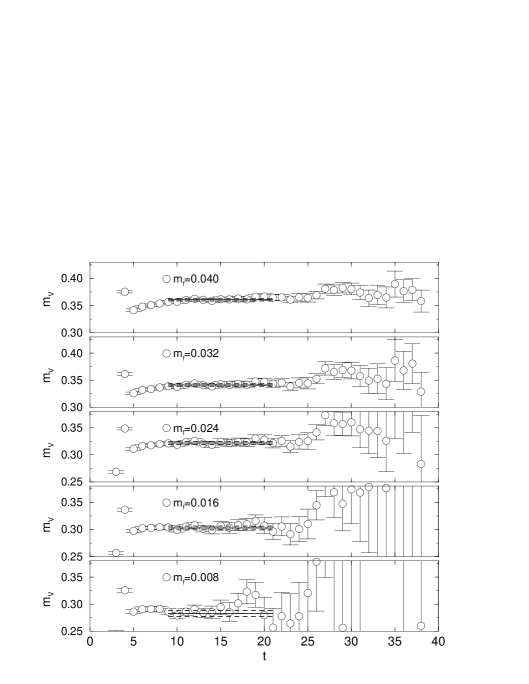
Figure 8: Vector meson effective mass plots for the DBW2, $\beta=1.22$ ensemble. Lines denote fitting results and indicate fitting range, central values and jackknife errors.

Figure 8 shows the vector meson effective masses with degenerate quark masses for DBW2 $\beta=1.22$. The lines denote results of fits to the hyperbolic function mentioned above and indicate the fitting range, central value, and magnitude of the jackknife error for each. Results for $m_{V}$ for each value of $m_{f}$ are collected in the second column of Table 4. The values of the ratio $m_{\rm PS}/m_{V}$ are also included in the third column of this table. Similar analyses were carried out in Refs. Aoki:2002vt and Blum:2000kn for DBW2 $\beta=1.04$ and Wilson $\beta=6.0$, respectively. Results for $m_{V}$ and $m_{\rm PS}/m_{V}$ are quoted from these references in the second and third columns of Table 5.

Examples of the chiral extrapolation for $m_{V}$ and $m_{\rm PS}^{2}$ with DBW2 $\beta=1.22$ are shown in Figs. 9 and 10, respectively. These figures contain masses obtained with non-degenerate quarks masses $m_{1}$ and $m_{2}$ as well. Data are plotted as $m_{f}=(m_{1}+m_{2}+2m_{\rm res})/2$. They appear to lie on a smooth line joining the degenerate mass points. We take linear fitting functions for the pseudoscalar mass-squared and the vector mass,

$$m_{\rm PS}^{2} = c_{0}^{P}+c_{1}^{P}(m_{f}+m_{\rm res}),$$ (13)

$$m_{V} = c_{0}^{V}+c_{1}^{V}(m_{f}+m_{\rm res}).$$ (14)

Values of these parameters are tabulated in Table 3. These parameters were determined by minimizing an expression for $\chi^{2}$ in which off-diagonal terms in the covariance matrix were omitted. Such an uncorrelated fit will give an valid result but, if substantial correlations are present, will result in a somewhat larger statistical error and an unusually small value for $\chi^{2}$. Singularities in the full covariance matrix prevented our including the off-diagonal terms. Note, here $m_{\rm res}$ is not a free parameter, but is fixed to be the central values of the results from Eq. 8. Because of the small values of $m_{\rm res}$ in our simulations, we do not take the non-zero value of $c_{0}^{P}$ as an indication of explicit chiral symmetry breaking. As explained above and in detail in Ref. Blum:2000kn , both unsuppressed topological near-zero modes of the Dirac operator in quenched simulations and neglecting the quenched chiral logarithm can make demonstrating that $m_{\pi}$ is zero in the chiral limit difficult.

We have also computed the values of the bare strange quark mass $m_{s}$ and $J$-parameter for DBW2 ensembles and results are summarized in Table 7. The strange quark mass is found from

$$\frac{\sqrt{c^{P}_{0}+c^{P}_{1}(m_{s}/2+m_{\rm res})}}{c^{V}_{0}+c^{V}_{1}(m_{ud}+m_{\rm res})} = \frac{m_{K}}{m_{\rho}}=\frac{495\ {\rm MeV}}{770\ {\rm MeV}},$$ (15)

Here we simply set $m_{ud}=-m_{\rm res}$. The presence of a non-zero intercept $c_{0}^{P}$ for $m_{\rm PS}^{2}$ in Eq. 13 makes a more precise determination of $m_{ud}$ difficult. The overall effect of this approximation is an $\approx 1\%$ error in the determination of $m_{\rho}$. We extract the kaon $B$-parameter by interpolation to the physical point, $m_{K}=495$ MeV, which is equivalent to evaluating our data at the point $m_{f}=m_{s}/2$ determined from Eq. 15. The $J$-parameter is defined as in Ref. Lacock:1995tq

$$J=\frac{dm_{V}}{dm_{\rm PS}}m_{K^{*}}=\frac{c^{V}_{1}}{c^{P}_{1}}m_{K^{*}},$$ (16)

where $m_{K^{*}}=c^{V}_{0}+c^{V}_{1}(m_{s}/2+m_{\rm res})$.

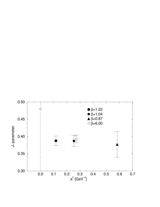
Figure 11: The $J$-parameter for DBW2 $\beta=1.22$ (filled circle), $1.04$ (filled square) and $0.87$ (filled triangle). The latter is reproduced from Ref. Aoki:2002vt . The open triangle represents the value obtained with Wilson $\beta=6.0$. Scaling violations are evidently less than the statistical errors.

The chiral symmetry of domain-wall fermions suppresses $O(a)$ discretization errors in low-energy observables, so the leading error is expected to be $O(a^{2})$. Thus, to study the scaling dependence of the $J$-parameter, we plot our results and the previous one for DBW2 $\beta=0.87$  Aoki:2002vt in Fig. 11 as a function of $a^{2}\ [{\rm GeV}^{-2}]$. These results are consistent with each other, showing that discretization errors are indeed small for this quantity. However, the quenched $J$-parameter value is much smaller than the experimental value, $m_{K^{*}}(m_{K^{*}}-m_{\rho})/(m_{K}^{2}-m_{\pi}^{2})=0.48$, by about 30%.

In making the comparison described above and shown in Fig. 11, we should emphasize that in addition to the quantified variation in lattice spacing, these points also correspond to varying gauge actions (Wilson and DBW2) and to different values of the domain-wall height, $M_{5}$. Since the coefficient of the $O(a^{2})$ correction to the $J$ parameter can depend on both the action and $M_{5}$, we should not attempt to fit the points in Fig. 11 to a single linear term in $a^{2}$. However, the agreement between these various values of $J$ certainly suggests considerable independence of the lattice spacing over a large range of lattice scales.

Before concluding this section, we present values for $m_{\rm PS}^{2}$ in physical units $[{\rm GeV}^{2}]$ in Table 8. In the following sections, these values will provide a physical horizontal scale, when quantities such as the decay constants, $K$–$\overline{K}$ matrix elements and $B_{K}$ are plotted as functions of quark mass. When $m_{\rm PS}^{2}$ is used in this way, the chiral limit will be identified as the point $m_{\rm PS}^{2}=0$. However, as was mentioned above and will be discussed further later, the slight difference between the points $m_{\rm PS}^{2}=0$ and $m_{f}=-m_{\rm res}$ when a simple linear fit is done (likely arising from the effects of near zero modes and neglecting the quenched chiral logarithm term) will introduce systematic errors at or below the 1% level.

IV PSEUDOSCALAR MESON DECAY CONSTANTS

In this section we discuss the calculation of the pseudoscalar decay constant $f_{\rm PS}$. In our Euclidean conventions, the definition of this quantity is

$$\left\langle 0\left|A_{4}\right|\rm PS\right\rangle=f_{\rm PS}\cdot m_{\rm PS},$$ (17)

where $\left|\rm PS\right\rangle$ stands for the zero-momentum pseudoscalar state. The experimental values for the pion and kaon states are $f_{\pi}\approx 130\ {\rm MeV}$ and $f_{K}\approx 160\ {\rm MeV}$.

We consider three separate lattice transcriptions of Eq. 17. In each case, rather than use the conserved axial current, we make use of the local, flavor non-singlet axial current. These two quantities are related by a finite renormalization constant, and we first discuss the extraction of the “bare” value of $f_{\rm PS}$, to which this factor has yet to be applied. The three formulae we use to extract the decay constant are

$$f^{(1)}_{\rm PS} = \frac{{\cal A}^{A_{4}P}_{\rm pw}}{\sqrt{\frac{m_{\rm PS}}{2}V{\cal A}^{PP}_{\rm ww}}},$$ (18)

$$f^{(2)}_{\rm PS} = \sqrt{\frac{2}{m_{\rm PS}\,V}\times\frac{{\cal C}^{A_{4}P}_{\rm pw}(t,t_{2})\,{\cal C}^{A_{4}P}_{\rm pw}(t,t_{1})}{{\cal C}^{PP}_{\rm ww}(t_{2},t_{1})}\Bigg{|}_{t_{1}\ll t\ll t_{2}}},$$ (19)

$$f^{(3)}_{\rm PS} = \sqrt{\frac{2{\cal A}^{PP}_{\rm ww}}{Vm_{\rm PS}}}\times\frac{{\cal C}^{A_{4}P}_{\rm pw}(t,t_{1})}{{\cal C}^{PP}_{\rm ww}(t,t_{1})}\Bigg{|}_{t\gg t_{1}},$$ (20)

where ${\cal C}^{A_{4}P}_{\rm pw}$ and ${\cal C}^{PP}_{\rm ww}$ are point-wall and wall-wall, axial-pseudoscalar and pseudoscalar-pseudoscalar correlation functions discussed in the previous section, $m_{\rm PS}$ is the common mass extracted from these correlation functions, and

$${\cal A}^{A_{4}P}_{\rm pw} = \frac{1}{2m_{\rm PS}}\left\langle 0\left|A_{4}\right|\rm PS\right\rangle\left\langle\rm PS\left|\chi_{P}^{\dagger}\right|0\right\rangle,$$ (21)

$${\cal A}^{PP}_{\rm ww} = \frac{1}{2m_{\rm PS}V}\left|\left\langle\rm PS\left|\chi_{P}\right|0\right\rangle\right|^{2},$$ (22)

are expressed as the product of correlation function amplitudes extracted from the same fit.

We take $f^{(1)}_{\rm PS}$ for our final value, using the same fitting range used to extract the pseudoscalar mass in the previous section. However, by also calculating $f^{(2)}_{\rm PS}$ and $f^{(3)}_{\rm PS}$ we are able to study the size of the systematic error that may arise from our choice of fit which may affect, for example, the amount of excited state contamination in the result. Another source of systematic error is unsuppressed topological near-zero modes of the Dirac operator in the presence of quenched gauge configurations. This contamination is elucidated in detail in Ref. Blum:2000kn , the salient points being that the contamination depends on the time separation of the operators, the particular construction of these operators (for example, whether a wall or point source is used), and the value of quark mass, lighter quarks showing a larger effect. The comparison between $f^{(1)}_{\rm PS}$ and $f^{(2)}_{\rm PS}$ is particularly interesting because the expression we use to calculate $B_{K}$ essentially contains $f^{(2)}_{\rm PS}$ in the denominator. $f^{(2)}_{\rm PS}$ tends to be contaminated by the topological near-zero mode since it is extracted from time slices closer than the case of $f^{(1)}_{\rm PS}$. As such, we use the same source positions and fitting ranges for the extraction of $f^{(2)}_{\rm PS}$ as we do for $B_{K}$, $(t_{1},t_{2})=(7,41)$ for DBW2 $\beta=1.22$ and $(5,27)$ for $\beta=1.04$ and Wilson $\beta=6.0$, with final values given by the fit over the ranges $19\leq t\leq 29$ and $14\leq t\leq 17$, respectively. For the purpose of this comparison we choose the fitting range for $f^{(3)}_{\rm PS}$ to be the same as that chosen for $f^{(1)}_{\rm PS}$.

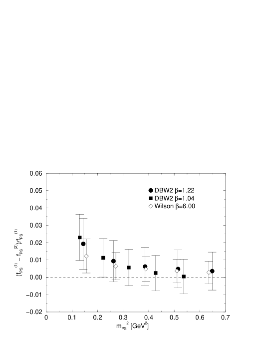
Figure 12: Deviation of $f^{(2)}_{\rm PS}$ from $f^{(1)}_{PS}$ as a function of $m_{\rm PS}^{2}\ [{\rm GeV}^{2}]$ for each parameter set, DBW2 $\beta=1.22$ (filled circles), $\beta=1.04$ (filled squares), and Wilson $\beta=6.0$ (open circles).

Table 9 shows the results for all three values of the decay constant for each quark mass. As can be seen, all these quantities agree within their quoted statistical errors. However, the statistical fluctuations of these quantities are correlated, so differences between these quantities may be resolved to a much higher precision than the quantities themselves. Figure 12 shows $(f^{(1)}_{\rm PS}-f^{(2)}_{\rm PS})/f^{(1)}_{\rm PS}$ as a function of $m_{\rm PS}^{2}$ for each ensemble. The central value of this difference monotonically increases and becomes roughly one percent at the kaon mass point $m_{\rm PS}=m_{K}=495$ MeV. Although data except at the lightest masses are consistent with zero within one standard deviation, it is important to note that the same behavior is observed for all independent ensembles. While it may suggest the effects of topological near-zero modes, more statistics are required for further study. In Section VI.2, we will discuss systematic error of $B_{K}$ which may originate from the ambiguity of $f_{\rm PS}$ stemming from the different methods of extraction.

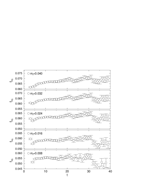
Figure 13: Effective lattice decay constant $f_{\rm PS}^{(1)}$ obtained from the pseudoscalar effective mass and corresponding amplitudes for DBW2 $\beta=1.22$. The mass $m_{f}$ increases from bottom to top. The fitting range $18\leq t\leq 31$ was used to extract $f_{\rm PS}^{(1)}$ for this case.

As mentioned previously, in the rest of this paper we employ $f^{(1)}_{\rm PS}$ as our result for the decay constant. In Figs. 13 and 14 effective values of $f^{(1)}_{\rm PS}$ are plotted versus time for DBW2 $\beta=1.22$ and $1.04$, respectively. While no significant time dependence is seen within the choice of fitting range for $\beta=1.04$, we find a monotonic decrease for smaller $t$ for $\beta=1.22$. However, the width of this variation is within the statistical error.

The renormalization constant of the local, flavor non-singlet, axial current is determined following the method in Ref. Blum:2000kn . As an example, the results for each quark mass for DBW2 $\beta=1.22$ are shown in Fig. 15. $Z_{A}$ is defined in the chiral limit which in practice is determined from a linear extrapolation to $m_{f}=-m_{\rm res}$. Results for $Z_{A}$ are summarized in Table 10.

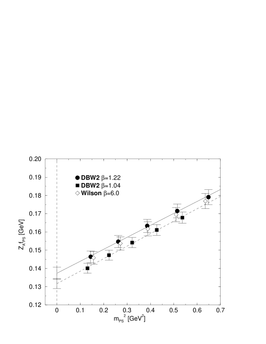
Figure 16: Renormalized values of the pseudoscalar decay constant as a function of $m_{\rm PS}^{2}\ [{\rm GeV}^{2}]$ for DBW2 $\beta=1.22$ (filled circle), $\beta=1.04$ (filled square), and Wilson $\beta=6.0$ (open diamond).

To determine the physical decay constants $f_{\pi}$ and $f_{K}$ we make use of NLO quenched chiral perturbation theory which suggests a simple linear quark mass dependence in the case of degenerate quarks  Sharpe:1992ft ; Bernard:1992mk . The results of these linear fits of the bare value $f_{\rm PS}$ are listed in Table 10. In the same table, the lattice values of decay constant $f_{\pi}^{\rm(latt)}$ and $f_{K}^{\rm(latt)}$ are listed. They are obtained by the extrapolation to the point $m_{\rm PS}=m_{\pi}=135$ MeV and the interpolation to $m_{\rm PS}=m_{K}=495$ MeV, respectively. In particular for the DBW2 results, we note that the lattice scale dependence of the renormalized value $Z_{A}f_{\rm PS}$ comes mainly from the scale dependence of $Z_{A}$. In Fig. 16 the renormalized decay constants $Z_{A}\!\cdot\!f_{\rm PS}$ are shown along with linear fits for DBW2 $\beta=1.22$ (solid line) and $\beta=1.04$ (dashed line). One observes agreement between DBW2 $\beta=1.22$ and Wilson $\beta=6.0$ values, but a discrepancy of roughly two standard deviations between DBW2 $\beta=1.22$ and $\beta=1.04$.

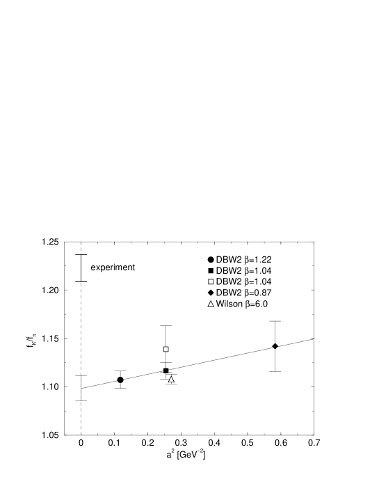
Figure 17: Scaling property of the ratio of physical pseudoscalar decay constants, $f_{K}/f_{\pi}$. The values for $\beta=0.87$ (filled diamond) and $\beta=1.04$ (open rectangle) are taken from Ref. Aoki:2002vt . The linear extrapolation to the continuum limit (solid line) uses the three new DBW2 data points: $\beta=1.22$ (filled circle), $\beta=1.04$ (filled square) and $\beta=0.87$ (filled diamond).

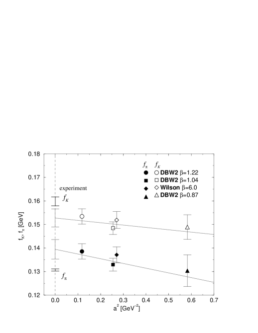
Figure 18: Scaling properties of the decay constants $f_{\pi}$ and $f_{K}$. The values for $\beta=0.87$ (triangles) are taken from Ref. Aoki:2002vt . Linear extrapolations to the continuum limit (solid lines) use the three DBW2 data points, $\beta=1.22$ (circles), $\beta=1.04$ (squares) and $\beta=0.87$ (triangles). Experimental results are also shown.

Renormalized decay constants $f_{\pi}=Z_{A}f_{\pi}^{\rm(latt)}$ and $f_{K}=Z_{A}f_{K}^{\rm(latt)}$ and their ratio $f_{K}/f_{\pi}=f_{K}^{\rm(latt)}/f_{\pi}^{\rm(latt)}$ are listed in Table 11. Since the last quantity contains neither the statistical errors of $a^{-1}$ nor the scaling dependence of $Z_{A}$, it may allow a more accurate study of scaling than the individual decay constants. Putting together our $f_{K}/f_{\pi}$ results with previous ones for DBW2 $\beta=1.04$ and $0.87$ Aoki:2002vt , which were obtained from a point-point correlation function on a non-doubled lattice, we find the scaling shown in Fig. 17. At $\beta=1.04$, our result is within the statistical error of the previous one. We extrapolate our DBW2 results and the previous $\beta=0.87$ value (filled symbols in the figure) linearly in $a^{2}$, (see the discussion at the end of the last section) and find the continuum limit value $f_{K}/f_{\pi}=1.098(13)$. A constant fit yields a consistent value with $\chi^{2}/$dof = 0.91. These results are roughly consistent with the one-loop analytic result $\approx 1.07$ of quenched chiral perturbation theory Bernard:1992mk and differ from the experimental results by several standard deviations. Similar plots are obtained for the individual decay constants as shown in Fig. 18 and results of the continuum extrapolation both with a linear and a constant fit are listed in Table 11. We again find consistent continuum values within the errors for both types of extrapolation.

V NON-PERTURBATIVE RENORMALIZATION for $B_{K}$

The value for $B_{K}$ depends on both renormalization scheme and scale. In this work, we will be quoting our final answer renormalized in the $\overline{\rm MS}$ scheme at $2$ GeV using the non-perturbative renormalization (NPR) technique of the Rome-Southampton group  Martinelli:1995ty . This technique has been found to be very successful, particularly when used in conjunction with domain-wall fermions, in which context it has been applied to the renormalization of fermion bilinear operators Blum:2001sr ; Dawson:1999yx , $B_{K}$ in previous calculations Dawson:1999yx ; Dawson:2000kh ; Blum:2001xb , and the four-quark operators in the $\Delta S=1$ effective Hamiltonian Blum:2001xb .

In the continuum, the parity-even operator of interest for the calculation of $B_{K}$,

$${\cal O}_{VV+AA}=(\bar{s}\gamma_{\mu}d)(\bar{s}\gamma_{\mu}d)+(\bar{s}\gamma_{5}\gamma_{\mu}d)(\bar{s}\gamma_{5}\gamma_{\mu}d)\,,$$ (23)

renormalizes multiplicatively. However, in a regularization in which chiral symmetry is broken, this operator may mix with four other four-quark operators; we must then solve the renormalization problem on the following basis of five operators:

$${\cal O}_{VV\pm AA} = (\bar{s}\gamma_{\mu}d)(\bar{s}\gamma_{\mu}d)\pm(\bar{s}\gamma_{5}\gamma_{\mu}d)(\bar{s}\gamma_{5}\gamma_{\mu}d),$$ (24)

$${\cal O}_{SS\pm PP} = (\bar{s}d)(\bar{s}d)\pm(\bar{s}\gamma_{5}d)(\bar{s}\gamma_{5}d),$$ (25)

$${\cal O}_{TT} = (\bar{s}\sigma_{\mu\nu}d)(\bar{s}\sigma_{\mu\nu}d)\ .$$ (26)

When using domain-wall fermions such mixing with wrong chirality operators should be strongly suppressed. However, as a consequence of their different chiral structure, chiral perturbation theory predicts that the contribution of these operators to $B_{\rm PS}$ will diverge in the chiral limit. As will be discussed in Section VI.2, even for the (relatively large) masses at which we are working, the contributions to $B_{\rm PS}$ from these wrong chirality operators are a few dozens of times larger than the one from ${\cal O}_{VV+AA}$, and so even a relatively small mixing coefficient may become numerically important in the final answer. In this work we address this problem by presenting both a theoretical argument to estimate the size of such terms, and the results of a numerical study. The question of possibly large mixing with wrong chirality operators in a domain wall fermion calculation of $B_{K}$ was raised in Ref. Becirevic:2004fw . The discussions presented here are intended to resolve this issue.

We may theoretically estimate the size of the mixing coefficients between ${\cal O}_{VV+AA}$ and the wrong chirality operators by applying the spurion field technique introduced in Ref. Blum:2001sr . The details of this analysis are presented in Appendix A; here we merely quote the result that, if we consider only the effects of the explicit chiral symmetry breaking of domain wall fermions, these mixing coefficients occur at $O(m_{\rm res}^{2})$. This represents a suppression factor which, in the presented calculations, is in the range $10^{-6}$ – $10^{-8}$, well below the level which could make a significant contribution to our result. If we also take into account the fact that we are working at finite quark mass, we would expect the leading contribution to the mixing coefficients to be of $O(m_{f}^{2})$. Such contributions will appear in any lattice formulation, and should be the dominant contribution from wrong chirality operators in any realistic calculation of $B_{K}$ using domain-wall fermions. In the following we numerically estimate the size of such terms.

We calculate the renormalization coefficients in a two step process: first we calculate the renormalization factor on the lattice in the RI/MOM-scheme, then make use of a continuum running/matching calculation to convert this into the $\overline{\rm MS}$-scheme. In this way, we avoid the use of lattice perturbation theory for which the convergence properties are problematic (requiring the use of mean field improvement). To apply the NPR technique we work in Landau gauge and construct the amputated $n$-point correlation functions of the operators of interest, $\Gamma^{(n){\rm latt}}_{\cal O}$, with external quark lines carrying large, off-shell momenta. The renormalization conditions may then be applied by requiring that suitable spin-color projections of this correlation function are equal to their tree case value. To be precise, for a general mixing problem involving $m$ operators, ${\cal O}_{i}$ ($i\in 1,\cdots,m$), each made up of $n$ quarks, we define the renormalized operators by the equation

$${\cal O}^{\rm ren}_{i}=Z_{ij}{\cal O}^{\rm latt}_{j}\,,$$ (27)

construct the amputated $n$-point correlation function, and apply, at a fixed configuration of external quark momenta, the condition

$$Z_{q}^{-n/2}Z_{ij}{\rm P}_{k}\left[\Gamma_{{\cal O}_{j}}^{(n){\rm latt}}(p\ ;\ a^{-1})\right]={\rm P}_{k}\left[\Gamma^{(n){\rm tree}}_{{\cal O}_{i}}\right]\,,$$ (28)

where ${\rm P_{k}}$ represents the application of a particular spin-color projection and a subsequent trace. (For details see Appendix B.) For a mixing problem with $m$ operators, $m$ independent projection operators need to be applied, however the precise choice will not effect the final renormalization factors. This is in contrast to the particular choice of gauge, quark mass, and the configuration of external quark momenta: these must be specified to fully define the renormalization condition (in all cases, we define our renormalization conditions to be in the chiral limit).

To calculate a renormalized value of $B_{K}$, the ratio of renormalization factors $Z_{Q^{(\Delta S=2)}}/Z_{A}^{2}$, which we refer to as $Z_{B_{K}}$, is required. As such, we calculated the amputated 3-point and 5-point Green functions for ${\cal O}=A_{\mu}$ and ${\cal O}=Q^{(\Delta S=2)}$, in each case using the same magnitude of momenta for all external quarks. As will be explained below, this is not the optimal choice of momenta for the lattice calculation. However, it is the only momenta configurations for which perturbative calculations of the matching between the RI/MOM- and $\overline{\rm MS}$-schemes exist. For the axial-vector operator the spin-color projection is achieved by tracing with $\gamma_{5}\gamma_{\mu}$. The ratio of renormalization factors, $Z_{q}^{-1}Z_{A}$, is then obtained from

$$Z_{q}^{-1}Z_{A}{\rm tr}[\Gamma^{(2){\rm latt}}_{A_{\mu}}(p;\ a^{-1})\gamma_{5}\gamma_{\mu}]=-48,$$ (29)

which is valid to $O(a^{2})$ even with non-zero $m_{\rm res}$ Blum:2001sr . The details of the projection operators used and derivation of the counterpart of Eq. 29 for the $\Delta S=2$ operators are given in Appendix B; in the following we will simply refer to the projected, amputated $n$-point correlation functions in terms of the matrices $\Lambda$ and $N$, defined as:

$$\Lambda_{ij} = {\rm P}_{j}\left[\Gamma_{{\cal O}_{i}}^{\rm latt}\right]$$ (30)

$$N_{ij} = {\rm P}_{j}\left[\Gamma_{{\cal O}_{i}}^{\rm tree}\right]\,.$$ (31)

Using these definitions Eq. 28 takes the form of a matrix equation

$$Z_{q}^{-2}Z_{ij}\Lambda_{jk}=N_{ik}\,.$$ (32)

In the first step of the numerical calculation, we calculate the quark propagator in coordinate space for each $m_{f}$ listed in Table 2. After performing a Fourier transformation into momentum space, we produce the quark propagator $G(p_{\rm latt})$, the treatment of which is described in Appendix B. We use a set of integer momenta $(n_{x},n_{y},n_{z},n_{t})$ on the lattice defined as

$$p_{\rm latt}=\left(\frac{2\pi}{L_{x}}n_{x},\frac{2\pi}{L_{y}}n_{y},\frac{2\pi}{L_{z}}n_{z},\frac{2\pi}{L_{t}}n_{t}\right),$$ (33)

where $L_{x}=L_{y}=L_{z}=24$ and $L_{t}=48$ for DBW2 $\beta=1.22$, and $L_{x}=L_{y}=L_{z}=16$ and $L_{t}=32$ for DBW2 $\beta=1.04$. We used 448 combinations of $(n_{x},n_{y},n_{z},n_{t})$ with $n_{x}$, $n_{y}$ and $n_{z}$ ranging from 0 to 3 and $n_{t}$ ranging from 0 to 6 for DBW2 $\beta=1.22$. For DBW2 $\beta=1.04$ we used $n_{x}$, $n_{y}$ in the range $-2$ to $2$, $n_{z}$ in the range 0 to 2 and $n_{t}$ in the range 0 to 4. These choices gave us a sufficient number of distinct momenta for our non-perturbative renormalization.

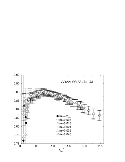
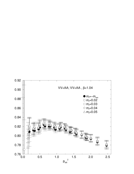
Figure 19: Renormalization factor $Z_{q}^{-2}Z_{Q^{(\Delta S=2)}}$ i.e. $Z_{q}^{-2}Z_{VV+AA,\ VV+AA}$ as a function of $p_{\rm latt}^{2}$ from DBW2 $\beta=1.22$ (left panel) and $\beta=1.04$ (right panel). For each momentum, data indicated by the open symbols are linearly extrapolated to the value (filled circles) in the chiral limit.

Results of the first diagonal element of $N\Lambda^{-1}$, $Z_{q}^{-1}Z_{VV+AA,VV+AA}$, versus $p_{\rm latt}^{2}$ are shown in Fig. 19 for each $m_{f}$, where the left/right panel is from DBW2 $\beta=1.22$/$1.04$ for each $m_{f}$ (open symbols) and chiral limit $m_{f}=-m_{\rm res}$ (filled circles).

The momentum and mass dependence of the data is expected to be classified into two regions as the operator product expansion would suggest. For low momenta, there should be significant contributions from hadronic effects. At larger momenta, this effect should be suppressed in an approximately power-law manner. For large enough momenta, there is a region in which the hadronic effects are negligible and the momentum dependence (running) is well described by perturbation theory. As we are working on the lattice, if we work at too large a momentum there will be significant contributions due to discretization errors. Therefore, the success of the NPR technique requires there to be a window of momenta for which contributions from both hadronic effects and discretization errors are small. Our data suggest this is the case. Namely, while at very low momenta there is significant momentum dependence, in momenta range ($\approx\ 2{\rm GeV}$) where we might expect that perturbation theory is valid there is only a mild momentum dependence. We use this range in the following to compare with the perturbative prediction.

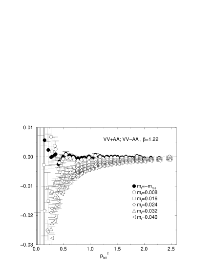
Figure 20: Same figure as Fig. 19 but for the renormalization factor $Z_{q}^{-2}Z_{VV+AA,\ VV-AA}$

Figure 20 shows the results of the off-diagonal element $Z^{-2}_{q}Z_{VV+AA,VV-AA}$ with the same organization as Fig. 19. For both the case of DBW2 $\beta=1.22$ and $1.04$, we obtain values in the chiral limit that are consistent with zero as a results of linear extrapolation with a reliable quality of fit. Figure 21 shows examples of mass dependences of $Z^{-2}_{q}Z_{VV+AA,VV-AA}$ for some fixed momenta both for $\beta=1.22$ (left) and $1.04$ (right). Data in this figure show linear behavior in conflict with the prediction of $O((m_{f}+m_{\rm res})^{2})$ dependence, implied by the discussion in Appendix A. This linear behavior should likely be interpreted as an error due to spontaneous chiral symmetry breaking. A nonzero value of $\left\langle\bar{q}q\right\rangle$ could cause systematic errors of $O\left((\Lambda_{\rm QCD}/p)^{6}\right)$ and $O\left((\Lambda_{\rm QCD}/p)^{3}\cdot(m_{f}+m_{\rm res})/p\right)$, which, for not large enough $p$, contribute as a sizable intercept and a linear term of the quark mass, respectively. This interpretation explains that, in Fig. 21, degree of the slopes in both panels and that of the intercept in the right panel decrease for larger values of $p_{\rm latt}$. Another possible source of the linear term is the dimension 7 operators which contain one derivative in a four-quark operator.

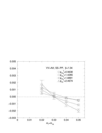
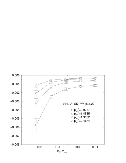
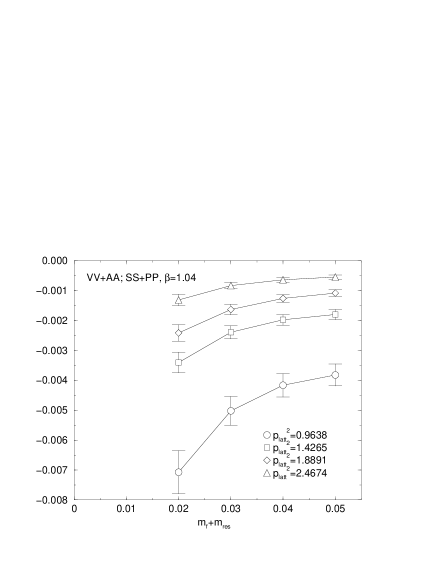
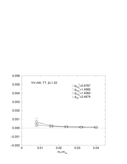
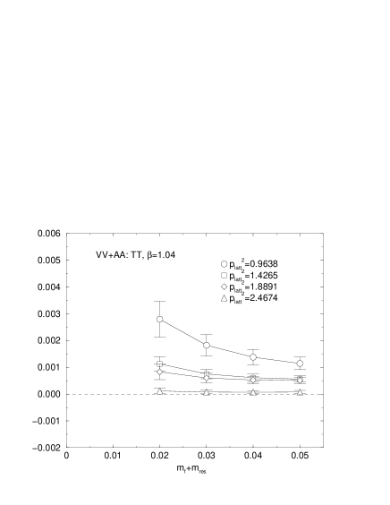
Figure 22: Renormalization factors $Z_{q}^{-2}Z_{VV+AA,\ j}$ as a function of $m_{f}+m_{\rm res}$ for several fixed values of $p_{\rm latt}^{2}$. From top to bottom, $j=SS-PP$, $SS+PP$ and $TT$ . Results for DBW2 $\beta=1.22$ and $1.04$ are in the left and right column, respectively.

Other off-diagonal elements $Z^{-2}_{q}Z_{VV+AA,SS-PP}$, $Z^{-2}_{q}Z_{VV+AA,SS+PP}$ and $Z^{-2}_{q}Z_{VV+AA,TT}$ do not allow a naive chiral extrapolation. For these factors, we plot $m_{f}$ dependences for several points of $p_{\rm latt}^{2}$ in Fig. 22. As can be seen, these elements increase in magnitude as quark mass is decreased. While it may seem counterintuitive that these measures of chiral symmetry breaking increase for small masses, this effect is well understood to be a result of the poor choice of momenta configurations for the renormalization condition: to be able to ignore hadronic contributions at large momenta, it is necessary that all the momenta in the problem are large compared to the hadronic scale, not just the external momenta. The choice of momenta that we have been forced to use to remain consistent with the perturbative matching calculation transfers no momentum through the operator. The contribution of any particle that this operator couples to is therefore only suppressed by that particle’s mass. Practically this is only a problem when the operator couples to a pseudo-Goldstone boson, the mass of which goes to zero in the chiral limit. While the presence of these “pion poles” greatly complicates any attempt to accurately extract the wrong chirality mixings, in this work we will content ourselves with placing a bound on the size of such contributions. As such we will extract the mixing coefficients using our heaviest values of the mass and largest values of the momentum. In this way we reduce the pion-pole contamination, while, at the same time, maximizing the $O(m_{f}^{2})$ contributions. As will be demonstrated in the next section, the resulting mixing coefficients are small enough that the wrong chirality operators can be safely neglected in our calculation of $B_{K}$, namely we calculate its renormalization factor as $Z_{B_{K}}^{\rm RI/MOM}=Z_{VV+AA}/Z_{A}^{2}$.

In Appendix C, we summarize the perturbative formulae for the renormalization group running and scheme matching. The authors of Refs. Ciuchini:1995cd ; Ciuchini:1997bw calculated a factor absorbing the scale and scheme dependence of the renormalization factor, $Z_{B_{K}}^{\rm RI/MOM}$, in NLO perturbation theory. Using this factor, we convert our results to the renormalization group independent (RGI) value,

$$\hat{Z}_{B_{K}}(N_{f})=w^{-1}_{\rm RI/MOM}(N_{f},p_{\rm latt}/a)\cdot Z^{\rm RI/MOM}_{B_{K}}(p_{\rm latt})\,.$$ (34)

This is related to the renormalization factor at a certain energy scale, $\mu$, in the $\overline{\rm MS}$-scheme using naive dimensional regularization by:

$$Z_{B_{K}}^{\rm\overline{MS}\ NDR}(N_{f},\ \mu)=w_{\overline{\rm MS}}(N_{f},\ \mu)\hat{Z}_{B_{K}}(N_{f})\,.$$ (35)

The functions $w_{\rm RI/MOM}$ and $w_{\overline{\rm MS}}$ are defined in Appendix C, and $p_{\rm latt}$ is the magnitude of the lattice momentum used in the Green’s function defining $Z^{\rm RI/MOM}_{B_{K}}$.

It should be noted that both Eq. 34 and Eq. 35 depend upon the number of active flavors. While the final result we are aiming at is an estimate of $B_{K}$ renormalized in full QCD (3 active flavors), our lattice calculations of the bare value of $B_{K}$ and the renormalization factors in the RI renormalization scheme are performed in the quenched approximation. While using Eq. 34 and Eq. 35 with either $N_{f}=0$ and $N_{f}=3$ – in any combination – would seem to be equally valid procedures (just different definitions of the quenched estimate for $B_{K}$ ), in this work we will consistently use $N_{f}=0$. One advantage of this approach is that it allows us to compare the observed scale dependence of the RI-scheme renormalization factors versus the perturbative prediction. In this way we are able to study the size of the associated systematic error.

In taking this approach, we must also employ a value of $\alpha_{S}$ in the quenched approximation. We obtain this using the two-loop formula given in Eq. 107, with $N_{f}=0$ and $\Lambda_{\rm\overline{MS}}^{(0)}=238$ MeV. This latter value is gained by taking the value of $r_{0}\Lambda_{\rm\overline{MS}}^{(0)}$ given by Capitani:1998mq and converting it to physical units using $r_{0}=0.5{\rm fm}$, the results of Guagnelli:1998ud , and our quoted value of the lattice spacing, as extracted from the chiral limit of the rho meson mass. This is the same approach employed in Blum:2001sr , where more details can be found. While the quenched coupling constant obtained from the value of the plaquette and rectangle Aoki:2002iq is another possible choice for $\alpha_{S}$, this choice changes the result of $Z^{\rm\overline{MS}\ NDR}_{B_{K}}$ by less than $0.1\%$.

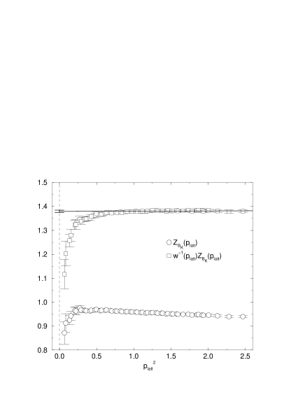
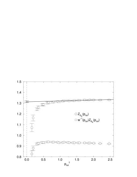
Figure 23: Renormalization factor of $B_{K}$ as a function of $p_{\rm latt}^{2}$ for DBW2 $\beta=1.22$ (left) and $\beta=1.04$ (right). In each panel, $Z_{B_{K}}$ (circles), $w^{-1}(p_{\rm latt})Z_{B_{K}}$ (squares) and its linear extrapolation using data for $p_{\rm latt}>1$ are shown.

The comparison between $Z_{B_{K}}^{\rm RI/MOM}$ and $\hat{Z}_{B_{K}}$ is shown in Fig. 23, for DBW2 $\beta=1.22$ (left panel) and DBW2 $\beta=1.04$ (right panel). One observes that $\hat{Z}_{B_{K}}$ is almost scale independent for $p_{\rm latt}\stackrel{{\scriptstyle>}}{{{}_{\sim}}}1$. Assuming the perturbation theory at NLO is good enough, the remaining small slope of $\hat{Z}_{B_{K}}$ is caused by discretization errors ($O((pa)^{2})$ effects). To remove these errors, we carry out a linear extrapolation in $p_{\rm latt}^{2}$ for $p_{\rm latt}>1$ and quote the values of intercept as $\hat{Z}_{B_{K}}$.

Our final results are

$$Z^{\rm\overline{MS}\ NDR}_{B_{K}}(N_{f}\!=\!0,\ \mu\!=\!2\,{\rm GeV})=\left\{\begin{array}[]{c}0.9901(36)\ \ \ {\rm DBW2}\ \beta=1.22\\ \\ 0.9427(54)\ \ \ {\rm DBW2}\ \beta=1.04\end{array}\right..$$ (39)

Note that it is possible to interpret the small but noticeable slope of the linear fit in the right panel of Fig. 23 as an error of the perturbation theory at lower momentum of $\approx 2$ GeV. Taking the constant fit instead, we obtain $\sim 1\%$ larger value for $\beta=1.04$. We may compare numbers in Eq. 39 against one-loop lattice perturbation theory calculation which has been done in Ref. Aoki:2002iq . Using measured values of the plaquette and rectangle as input, the perturbative renormalization factors are

$$Z^{\rm\overline{MS}\ NDR}_{B_{K}}(N_{f}\!=\!0,\ \mu\!=\!2\,{\rm GeV})=\left\{\begin{array}[]{c}0.9775\ \ \ {\rm DBW2}\ \beta=1.22\\ \\ 0.9493\ \ \ {\rm DBW2}\ \beta=1.04\end{array}\right.,$$ (43)

both of which lie close to the non-perturbative values. We find it reassuring that these two quite different methods lead to results agreeing to better than 2%

VI KAON $B$-PARAMETER

VI.1 Chiral behavior of $K$–$\overline{K}$ matrix element

Before presenting our results for $B_{K}$, it is important to check the chiral behavior of the $K$–$\overline{K}$ matrix element of $Q^{(\Delta S=2)}$. We calculate the three point correlation function with degenerate quarks and find a suitable plateau for $t_{1}\ll t\ll t_{2}$ to extract the desired matrix element:

$$\left\langle\overline{\rm PS}\left|Q^{(\Delta S=2)}\right|\rm PS\right\rangle = \frac{\left\langle 0\left|\chi_{P}(t_{2})Q^{(\Delta S=2)}(t)\chi_{P}^{\dagger}(t_{1})\right|0\right\rangle}{{\cal C}^{PP}_{\rm ww}(t_{2},t_{1})}\Biggr{|}_{t_{1}\ll t\ll t_{2}}\times 2m_{\rm PS}.$$ (44)

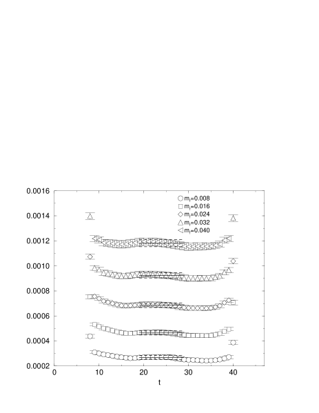
Figure 24: The time-dependence of the numerator of the left-hand-side of Eq. 44 for the DBW2 $\beta=1.22$ data set. The plotted horizontal lines indicate both the fitting range and the upper and lower limits of the resulting fitting value.

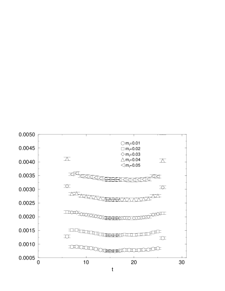
Figure 25: The same quantity as plotted in Fig. 24 except for the DBW2 $\beta=1.04$ data set.

As mentioned earlier, the sink and source locations were chosen to be $(t_{1},t_{2})=(7,41)$ for DBW2 $\beta=1.22$ and $(5,27)$ for $\beta=1.04$ and Wilson $\beta=6.0$. Results from a constant fit to the plateau of the matrix element for each $m_{f}$ in the fitting ranges $19\leq t\leq 29$ (DBW2 $\beta=1.22$) and $14\leq t\leq 17$ (DBW2 $\beta=1.04$ and Wilson $\beta=6.0$) are listed in Table 12. If a single intermediate state contributes to the matrix element in the numerator of the right-hand-side of Eq. 44, this quantity will be independent of the intermediate time $t$. This is demonstrated in Figs. 24 and 25 which show this quantity as a function of $t$ for each of the masses analyzed. Both graphs show an apparent plateau region which could be as large at 17 time units for $\beta=1.22$ and 10 time units for $\beta=1.04$. It seems likely that in the fitting range chosen contamination for excited states should be below a few percent.

In quenched chiral perturbation theory this matrix element, expanded in powers of $m_{\rm PS}^{2}$ up to $O(m_{\rm PS}^{4})$, is given by Sharpe:1992ft :

$$\left\langle\overline{\rm PS}\left|Q^{(\Delta S=2)}\right|\rm PS\right\rangle=a_{1}m_{\rm PS}^{2}\left[1-\frac{6}{(4\pi f)^{2}}m_{\rm PS}^{2}\ln\frac{m_{\rm PS}^{2}}{\Lambda_{\chi}^{2}}\right]+a_{2}(m_{\rm PS}^{2})^{2},$$ (45)

where, following the discussion in Section III, we neglect both the quenched chiral log and the chiral log terms in $m_{PS}^{2}$. Since the expansion starts at $O(m_{\rm PS}^{2})$, this matrix element vanishes in the chiral limit, $m_{\rm PS}^{2}=0$. Another characteristic of Eq. 45 is that the ratio of the coefficients of the leading term and the chiral-log term is determined solely by $f$, the decay constant in the chiral limit. It is interesting to examine our data in light of these expectations from quenched chiral perturbation theory. For this purpose, we carried out the two-parameter fit to Eq. 45 using for $f$ the product of chiral limit value $f_{0}$ and $Z_{A}$ listed in Table 10. Figure 26 shows $\left\langle\overline{\rm PS}\left|Q^{(\Delta S=2)}\right|\rm PS\right\rangle$ in lattice units and the fitting curve from Eq. 45 for DBW2 $\beta=1.22$ (left panel) and $\beta=1.04$ (right panel). We also used the fitting functions

$$\left\langle\overline{\rm PS}\left|Q^{(\Delta S=2)}\right|\rm PS\right\rangle = a_{0}+a_{1}m_{\rm PS}^{2}\left[1-\frac{6}{(4\pi f)^{2}}m_{\rm PS}^{2}\ln\frac{m_{\rm PS}^{2}}{\Lambda_{\chi}^{2}}\right]+a_{2}(m_{\rm PS}^{2})^{2}$$ (46)

and

$$\left\langle\overline{\rm PS}\left|Q^{(\Delta S=2)}\right|\rm PS\right\rangle = a_{1}m_{\rm PS}^{2}+a_{2}(m_{\rm PS}^{2})^{2}+a_{3}(m_{\rm PS}^{2})^{2}\ln\frac{m_{\rm PS}^{2}}{\Lambda_{\chi}^{2}}$$ (47)

to examine possible explicit chiral symmetry breaking effects through the magnitude of $a_{0}$ and to compare the result for $a_{3}/a_{1}$ to the chiral perturbation theory prediction of $-6/(4\pi f)^{2}$. As listed in Table 13, all three fitting functions in Eqs. 45, 46 and 47 with $\Lambda_{\chi}=1$ GeV fit our data equally well. Results for $a_{1}$ and $a_{2}$ are consistent among the fits, and $a_{0}$ in Eq. 46 is consistent with zero. The latter agrees with previous quenched domain-wall fermion calculations that showed $\left\langle\overline{\rm PS}\left|Q^{(\Delta S=2)}\right|\rm PS\right\rangle$ vanishes in the chiral limit, $m_{\rm PS}^{2}=0$, or $m_{f}=-m_{\rm res}$, to good accuracy AliKhan:2001wr ; Blum:2001xb . The same is true of our recent calculation of $B_{K}$ in the two-flavor theory Aoki:2004ht . Furthermore, $a_{3}/a_{1}$ from Eq. 47 reproduces the analytic result $-6/(4\pi f)^{2}$ fairly well, as did our previous calculation using the Wilson gauge action at $\beta=6.0$ Blum:2001xb . This was not the case in Ref. AliKhan:2001wr though in that study the authors did not examine $\left\langle\overline{\rm PS}\left|Q^{(\Delta S=2)}\right|\rm PS\right\rangle$ directly, but a ratio $\left\langle\overline{\rm PS}\left|Q^{{}^{(\Delta S=2)}}\right|\rm PS\right\rangle/\left\langle 0\left|P\right|{\rm PS}\right\rangle^{2}$, where $P$ is the pseudoscalar density. While it is reassuring that our data fits standard quenched chiral perturbation theory so well, it should be kept in mind that the analysis presented here includes quite heavy pseudo-scalar masses which may lie above the region where chiral perturbation theory is valid and has neglected quenched chiral logarithms and finite volume effects which may distort the lightest mass points.

VI.2 Results for $B_{K}$

Let us now discuss our results for the kaon $B$-parameter, $B_{K}$ defined in Eq. 1. Following our earlier conventions for the decay constant and pseudoscalar mass, we will use the notation $B_{\rm PS}$ for this $\Delta S=2$ amplitude evaluated for pseudoscalar states with a general meson mass, $m_{\rm PS}$. The parameter $B_{K}$ will be used when $m_{\rm PS}=m_{K}$: $B_{K}=B_{\rm PS}(m_{K})$. In the lattice calculation of $B_{\rm PS}$ we deal with the same three-point correlation function as in the previous subsection, but in a ratio with two factors of the wall-point correlation function ${\cal C}^{A_{4}P}_{\rm pw}$,

$$B_{\rm PS}=\frac{\left\langle 0\left|\chi^{\dagger}(t_{2})Q^{(\Delta S=2)}(t)\chi^{\dagger}(t_{1})\right|0\right\rangle}{\frac{8}{3}{\cal C}^{A_{4}P}_{\rm pw}(t,t_{2}){\cal C}^{A_{4}P}_{\rm pw}(t,t_{1})}\Biggr{|}_{t_{1}\ll t\ll t_{2}} = \frac{\left\langle\overline{\rm PS}\left|Q^{(\Delta S=2)}\right|\rm PS\right\rangle}{\frac{8}{3}m^{2}_{{\rm PS}}\left(f^{(2)}_{\rm PS}\right)^{2}}.$$ (48)

Here we suppress the appropriate $(\rm latt)$ superscript, $B_{\rm PS}^{(\rm latt)}\rightarrow B_{\rm PS}$.

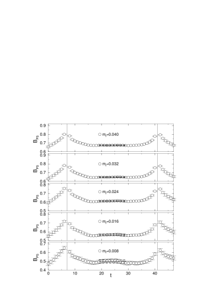
Figure 27: Time dependence of $B_{PS}$ for $\beta=1.22$. Panels from bottom to top correspond to increasing $m_{f}$. The horizontal bars in each plot indicate the range used in the constant fit, the results for the central value (solid line) and the jackknife error (dashed lines).

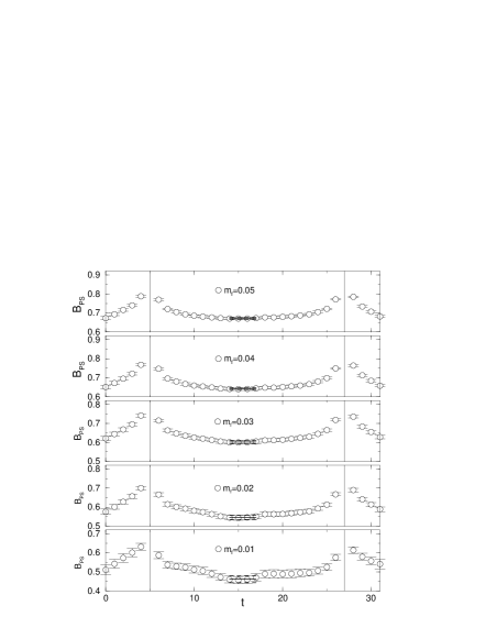
Figure 28: Time dependence of $B_{PS}$ for $\beta=1.04$. The organization is same as in Fig. 27.

Plateaus for this ratio for each value of $m_{f}$ are shown in Fig. 27 for DBW2 $\beta=1.22$ and in Fig. 28 for $\beta=1.04$ (the quark mass increases from bottom to top in each figure). The solid and dashed lines in each plot indicate the fitting range used ($19\leq t\leq 29$ for $\beta=1.22$ and $14\leq t\leq 17$ for $\beta=1.04$) and the results for a constant fit that are also listed in Table 14. As is suggested by Figs. 27 and 28, these fitting ranges are chosen quite conservatively and could likely be made larger without significant contamination from higher mass, excited states. In fact, choosing a larger fitting range yields consistent results. For example, for our lightest masses, increasing the fitting range to $17\leq t\leq 31$ for $\beta=1.22$ decreased the result by 1% while for $\beta=1.04$ the enlarging the fitting range to $12\leq t\leq 19$ increased the result by 2.5%, both within one standard deviation of the results quoted in Table  14.

In Ref. Blum:2001xb , we chose a different method to determine $B_{\rm PS}$, computing separately the numerator and denominator of Eq. 48 and then evaluating their ratio. In the present case, that method and the one used here give results which agree within statistical errors. Another variant of our method replaces the quantity $f^{(2)}_{\rm PS}$ formally contained in the denominator of Eq. 48, with the alternative $f^{(1)}_{\rm PS}$ which is computed in Section IV. However, as can be seen in Fig. 12, the difference between the two is always less than two percent, even for the lightest $m_{f}$, and usually smaller than one percent.

The counterpart of Eqs. 45 and 47 for $B_{K}$ is

$$B_{\rm PS} = \xi_{0}\left[1-\frac{6}{(4\pi f)^{2}}m^{2}_{\rm PS}\ln\frac{m_{\rm PS}^{2}}{\Lambda_{\chi}^{2}}\right]+\xi_{1}m_{\rm PS}^{2},$$ (49)

and

$$B_{\rm PS} = \xi_{0}+\xi_{1}m_{\rm PS}^{2}+\xi_{2}m^{2}_{\rm PS}\ln\frac{m_{\rm PS}^{2}}{\Lambda_{\chi}^{2}},$$ (50)

respectively Sharpe:1992ft . For degenerate quarks, these have the same form as in the theory with sea quarks Golterman:1997st , i.e. there are no quenched chiral logarithms in $B_{\rm PS}$ because of the cancellation of such terms between numerator and denominator in Eq. 48. Values of the fitting parameters for these functions are given in Table 15. As seen in this table, we find both fits are equivalent, with the $\beta=1.04$ case showing the closest agreement.

We also constructed $B_{\rm PS}$ from $\left\langle\overline{\rm PS}\left|Q^{(\Delta S=2)}\right|\rm PS\right\rangle$ calculated as described in the previous subsection and $f^{(2)}_{\rm PS}$ obtained from a constant fit to the plateau in $t$ for the ratio ${\cal C}^{A_{4}P}_{\rm pw}(t,t_{2}){\cal C}^{A_{4}P}_{\rm pw}(t,t_{1})/{\cal C}^{PP}_{\rm ww}(t_{2},t_{1})$. While the central value of the result changes by less than 0.2%, the jackknife error on the ratio increases by $\sim 70$% compared to the jackknife error coming directly from the use of Eq. 48.

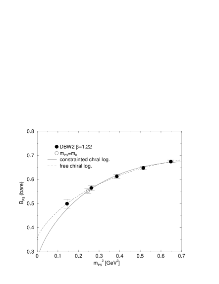
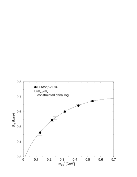
Figure 29: $B_{PS}$ as a function of $m_{PS}^{2}\ [{\rm GeV}^{2}]$ for DBW2 $\beta=1.22$ (left) and $\beta=1.04$ (right). In each panel, solid curves are the results of the fit to Eq. 49. Dashed curve in the left panel denotes the fit to Eq. 50.

In Fig. 29, we plot bare values of $B_{\rm PS}$ versus $m_{\rm PS}^{2}$ (DBW2 $\beta=1.22$ and $1.04$ for the left and right panels, respectively). The solid and dashed curves denote fits to Eqs. 49 and 50 which, for DBW2 $\beta=1.22$, somewhat differ in contrast with the case of the $\left\langle\overline{\rm PS}\left|Q^{(\Delta S=2)}\right|\rm PS\right\rangle$ matrix element where they were almost on top of each other. We found that this difference does not depend on the choice of fitting range. Repeating the same analysis for both $\beta$ values using the larger fitting ranges described above did not change the situation. Since we extract $B_{K}$ from an interpolation of $B_{\rm PS}$ to the kaon mass (around the data point for second lightest mass), the choice of fitting function makes little difference in the value of $B_{K}$, as discussed below. In the absence of a compelling reason to choose one over the other, we pick Eq. 49 to be consistent with chiral perturbation theory.

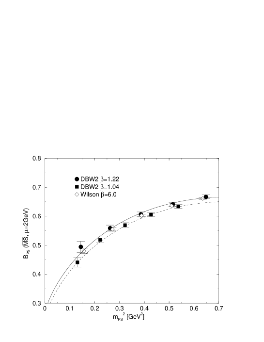
Figure 30: $B_{PS}$ renormalized in $\overline{\rm MS}$ NDR scheme at $\mu=2$ GeV as a function of $m_{\pi}^{2}\ [{\rm GeV}^{2}]$. Filled symbols are from DBW2 $\beta=1.22$ (circle) and $1.04$ (square). Fitting curves indicated by the solid and dashed lines respectively are added to them. Open diamonds are Wilson $\beta=6.0$ data.

Interpolation to the physical point, $m_{\rm PS}=m_{K}=495$ MeV, yields the lattice values of $B_{K}^{(\rm latt)}$ listed in the last column of Table 15 and indicated by the open symbols in Fig. 29. Though we use Eq. 49 to obtain $B_{K}^{(\rm latt)}$ in the rest of this article, the difference from using Eq. 50 is always less than 1%. After multiplying $B_{\rm PS}$ by $Z_{B_{K}}^{\rm\overline{MS}\ NDR}(N_{f}=0,\,\mu=2\ {\rm GeV})$ in Eq. 39, we can directly compare the renormalized values from each ensemble as shown in Fig. 30, where filled symbols denote DBW2 $\beta=1.22$ (circles) and $\beta=1.04$ (squares) and open diamonds, Wilson $\beta=6.0$. Fitted curves corresponding to Eq. 49 for DBW2 $\beta=1.22$ (solid) and $\beta=1.04$ (dashed) are also shown in the figure. Since the points do not lie along identical curves, there are evidently lattice spacing errors remaining in our determination of $B_{K}$.

As was discussed in Section V, a possible systematic error that may contaminate $B_{K}$ is mixing with wrong chirality operators through renormalization:

$$B_{K}^{\rm(ren)}=B_{K}+\sum_{i}Z_{VV+AA,i}/Z_{A}^{2}\cdot B_{i}^{\rm(latt)},$$ (51)

where the $B$-parameters for the wrong chirality operators, ${\cal O}_{i}={\cal O}_{VV-AA},\ {\cal O}_{SS\pm PP},$ and ${\cal O}_{TT}$, are defined as

$$B_{i}^{(\rm latt)}=\frac{\left\langle\overline{\rm PS}\left|{\cal O}_{i}\right|\rm PS\right\rangle}{\frac{8}{3}f_{\rm PS}^{2}m_{\rm PS}^{2}}\,.$$ (52)

In Section V we pointed out the large, $O(m_{\rm res}^{2})$ suppression of this contamination. Here, we press our point by a numerical demonstration.

For DBW2 $\beta=1.04$, we have calculated all of these $B$-parameters following the same methods used for $B_{\rm PS}$. The results are listed in Table 16 and shown in Fig. 31. The magnitudes of the $B$-parameters for these wrong chirality operators are less than two orders of magnitude larger than $B_{\rm PS}$, even for quark masses of $\approx m_{s}/4$. This makes their effects at $m_{s}/2$ very small, given the further $O(m_{\rm res}^{2})$ suppression present in the mixing coefficients. The difficulties in accurately determining these miniscule mixings were outlined in Section V, namely we can not measure them accurately with our current techniques. As a gross overestimate of the size of these mixings, we measured their values at the largest momentum $p_{\rm latt}^{2}=2.4674$ and the heaviest quark mass $m_{f}=0.05$ and find contamination from each ${\cal O}_{i}$ is no larger than $0.01$. Moreover, cancellation between the wrong chirality terms in Eq. 51 likely makes the net contamination even smaller. Thus, we conclude that in our determination of $B_{K}$, the contributions from the wrong chirality operators are well below our statistical error.

Results for $B_{K}^{\overline{\rm MS}\ {\rm NDR}}(\mu\!=\!2\,{\rm GeV})\equiv Z_{B_{K}}(N_{f}\!=\!0,\mu\!=\!2\,{\rm GeV})\cdot B_{K}^{\rm(latt)}$ and $\hat{B}_{K}\equiv\hat{Z}_{B_{K}}(N_{f}\!=\!0)\cdot B_{K}^{\rm(latt)}$ are collected in Table 17, where we enumerate perturbatively (PR) as well as non-perturbatively (NPR) renormalized values. Results of a linear extrapolation and a constant fit to the continuum limit for each quantity are listed in the first two rows. As mentioned in Section V, while $B_{K}^{\overline{\rm MS}\ {\rm NDR}}$ is almost independent of our choice for $\Lambda^{(0)}_{\overline{\rm MS}}$, $\hat{B}_{K}$ is significantly sensitive. For that reason, we focus on the result for the former quantity in the following.

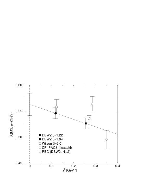
Figure 32: Summary of our results for $B_{K}^{\rm\overline{MS}\ NDR}(\mu=2\ {\rm GeV})$ renormalized with $N_{f}=0$ as a function of the lattice spacing squared. The filled circles are our results and the open symbols are quoted from previous works AliKhan:2001wr ; Blum:2001xb . Open diamond is the $N_{f}=2$ result obtained in Ref. Aoki:2004ht .

Our results for $B_{K}^{\overline{\rm MS}\ {\rm NDR}}(\mu\!=\!2\,{\rm GeV})$ are shown in Fig. 32 as a function of $a^{2}$ along with results from Ref. Blum:2001xb and the results obtained by the CP-PACS collaboration AliKhan:2001wr using domain-wall fermions with parameters similar to ours ($a^{-1}\!=$ 2.87 GeV, $24^{3}\times 60$ sites, $L_{s}=16$ and $a^{-1}$ = 1.88 GeV, $16^{3}\times 40$ sites, $L_{s}=16$). The main difference from our calculation is their use of the Iwasaki gauge action and perturbative renormalization of $B_{\rm PS}^{\rm(latt)}$. At $a^{-1}\approx 2$ GeV, results from the two collaborations differ by roughly two standard deviations: $B_{K}^{\overline{\rm MS}\ {\rm NDR}}(\mu\!=\!2\,{\rm GeV})=0.564(14)$ (CP-PACS) and $0.532(11)$ (Wilson $\beta=6.0$), $0.524(11)$ (DBW2 $\beta=1.04$). The two results are even more consistent at the smaller lattice spacing.

The discussion of the continuum extrapolation of the $J$-parameter and the decay constants in previous sections is valid here as well. While the result of constant fit in Table  17 is quite acceptable with a $\chi^{2}$/dof of 1.8, we use the linear extrapolation, shown in Fig. 32, to obtain our final result because we have no a priori reason to expect the $a^{2}$ term to be absent. This linear extrapolation is done by connecting our two data points and the error for the continuum limit is obtained by quadrature. We obtain the final result:

$$B_{K}^{\overline{\rm MS}\ {\rm NDR}}(\mu=2\ {\rm GeV})=0.563(21)(39),$$ (53)

where first error is statistical and the second systematic, which is discussed in the next subsection.

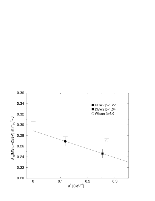
Figure 33: The continuum extrapolation of $B_{\rm PS}$ evaluated in the chiral limit.

Finally we give a result for $B_{\rm PS}$, evaluated in the chiral limit and then extrapolated to the continuum limit: $B_{\rm PS}^{\overline{\rm MS}\,{\rm NDR}}(m_{\rm PS}=0,\,\mu=2\,{\rm GeV})=0.289(18)$, where we do not attempt to determine the systematic errors for this value because of the sizable uncertainties associated with evaluating the chiral limit from our data. As is displayed in Fig. 33, we again see relatively mild dependence on the lattice spacing. This result is based on the chiral fits using the known chiral logarithm given in Eq. 49 and tabulated in Table 15. Here we do not compare with the CP-PACS result for this quantity because their use of an un-constrained fit to the chiral logarithm, which we are able to avoid, introduces large uncertainties in the chiral limit.

VI.3 Estimate of systematic errors

All of the statistical errors obtained earlier in this paper have been assigned using standard jackknife procedures and should reflect the variations that would be seen if our Monte Carlo calculations were simply repeated and analyzed in an identical fashion. (Of course, one should recognize that these errors, obtained from a finite data set are themselves subject to error.) Less certain but equally important are the errors in our results that come from systematic limitations in the calculation. These may be crudely divided into two types. First and easiest to determine are those associated with our methods of analysis. Our choice of plateau region, the procedure for chiral extrapolation or interpolation and our method for taking the continuum limit are good examples. Here the calculation should show consistency with the theoretical ideas being used in the analysis and the variation in the result between different approaches should indicate the level of systematic error. Of course, if the theoretical framework describes the data poorly or contains many parameters, a reliable estimate of systematic errors may not be possible.

The second type of error reflects ingredients which are missing in the calculation. If only a single volume or lattice spacing is used, the errors associated with finite volume or finite lattice spacing cannot be determined from the calculation at hand. Similarly the errors induced by the quenched approximation cannot be known if no full-QCD calculations have been performed. While one may “estimate” an expected error by comparing with more extensive calculations of other quantities, such estimates often reduce to an exercise in wishful thinking. However, for the case of $B_{K}$ there are now many results reported from other $B_{K}$ calculations which either independently, or by comparison with the work presented here, provide reasonably direct information about all of the important sources of error.

In the discussion to follow and the final results quoted we attempt to estimate the size of these systematic effects based on the calculations presented in this paper and the results of other work. These ”systematic errors” are not intended to be upper bounds on the size of these systematic effects but an estimate of their likely size. Thus, in performing such estimates we will not add cautionary inflation factors as would be appropriate if we were attempting to deduce reliable upper bounds on these errors. Rather we believe that we can extract the greatest value from this calculation by attempting to directly determine the suggested size of these effects. Attempting to determine the errors on these estimates (finding ”errors on errors”) or to establish reliable upper bounds on the size of these effects is beyond the scope of the present work. Each possibly important source of systematic error will now be discussed in turn and the results summarized in Table 18.

Extraction of $K-\overline{K}$ matrix element. As was discussed in Section VI.2, there is systematic uncertainty inherent in our method of determining the ratio $B_{\rm PS}$ defined by Eq. 48 associated with the choice of fitting region. Specifically, if the fitting range includes times too close to the source or sink, the resulting value for $B_{\rm PS}$ may receive contamination from excited states. This was studied quantitatively by comparing two choices of fitting region where variation in the result for $B_{\rm PS}$, on the order of the statistical uncertainty was seen. In this situation, our choice of fitting range determines the character of this error. If we had chosen a large fitting range, risking such excited state contamination, we would see a smaller statistical error (reflecting the larger number of points in our fit) but a larger systematic error. The systematic error would be determined by a comparison with the smaller fitting range and would likely be dominated by the statistical error from the smaller fitting range. In the approach we have taken, using the safer, smaller fitting range, the error is essentially statistical since we are well away from a region where excited state contamination might be expected. As might be deduced from Fig. 24, the data shows so little time dependence, that it is not possible to reliably extract the mass of a possible excited state from the relevant correlation functions. Instead, we estimate this possible contamination by evaluating $e^{-\Delta mt}$ for t corresponding to the 11 lattice spacings, the distance between our measurements and the source. If we choose $\Delta m=1$ GeV as the gap between our K meson and the first excited state with the same quantum numbers, this suggests an upper bound on this possible percentage contamination of 3%.

Determination of $f_{K}$. Since $B_{K}$ is the ratio of a $K-\overline{K}$ matrix element divided by $f_{K}^{2}$, the systematic error in determining the kaon decay constant must enter our result for $B_{K}$. This was discussed in Section IV where, by carefully comparing statistically correlated quantities, we were able to recognize a systematic difference between different methods for determining $f_{K}$, possibly caused by unsuppressed near zero modes. These differences were on the level of 1% for second to the lightest mass which has the greatest effect on the determination of $B_{\rm PS}$ at the Kaon mass. Thus, this source of error is listed in Table 18 as a 1% effect.

Kaon mass. Although $B_{K}$ is dimensionless, it is obtained by interpolation to the point $m_{\rm PS}=m_{K}$ and therefore depends on our choice for the K meson mass. While we have determined the Kaon mass directly in lattice units quite accurately ($\sim 1\%$, see Tables 4 and 5) there is further uncertainty in determining the lattice scale in physical units, especially in a quenched calculation. Following past practice, we have determined the lattice scales given in Table 7 from the $\rho$ mass. However, the fact that the $\rho$ meson is a stable state in this calculation but is an unstable particle in Nature with a width to mass ratio of 20%, suggests that this may introduce significant systematic errors. The dimensionful decay constants $f_{\pi}$ and $f_{K}$ provide alternative values for the lattice spacing. The discrepancies between their continuum limits (using $m_{\rho}$ to set the lattice scale) given in Table 11 and experiment provides a simple $\sim 6\%$ estimate of this source of systematic error in the choice of value for $m_{K}$. Referring to the dependence of $B_{K}$ on the input kaon mass shown in Eq. 50 or extracted from Tables 4, 5 and 14, we conclude that a 6% error in $m_{K}$ propagates into a 3% error in $B_{K}$.

We can also use the static quark potential to set the lattice scale. This was done for the quenched lattice configurations studied here by Hashimoto and Izubuchi in Ref. Hashimoto:2004rs . The comparison between the lattice scale determined from $m_{\rho}$ and that implied by a choice for the Sommer scale of $r_{0}=0.5$ GeV is given in their Table 1, showing agreement on the 6-9% level, roughly consistent with our 6% estimate. As mentioned above, much of the difficulty in determining the lattice scale from experiment comes from the quenched approximation and hence may already be represented in the error associated with the quenched approximation discussed below. However, we have adopted the conservative approach of listing the effects on $B_{K}$ of this resulting uncertainly in $m_{K}$ as a separate error.

Operator normalization (NPR). The non-perturbative renormalization of the left-left operator $Q^{(\Delta S=2)}$ as it appears in Eq. 1 provides a case where we expect the RI/MOM procedure of the Rome-Southampton group to be particularly accurate. The somewhat less precise wave function renormalization constant $Z_{q}$ cancels in this ratio and, as can be seen from Figs. 23, there is a large kinematic region, $1\leq p_{\rm latt}$, free of infrared QCD effects. We believe that the principle source of systematic error in the determination of $Z_{B_{K}}$ is the presence of lattice spacing errors in this region. As discussed in Section V, we attempt to remove these errors by identifying and subtracting an $(p_{\rm latt}a)^{2}$ term. This introduces a 1% change which we will adopt as an estimate of the systematic error in this determination of $Z_{B_{K}}$.

Operator normalization (PT). As is discussed in Section V, a final perturbative step is needed to convert $B_{K}$ defined in the RI/MOM scheme to the more conventional, perturbatively defined $\rm\overline{MS}\;NDR$ scheme. This correction factor is 1 at tree level while the NLO correction, $O(\alpha_{S})$, introduces a 1.3% change. In order to provide a proper estimate of the omitted $O(\alpha_{S}^{2})$ term we would need either a two loop result, which is not available, or a step-scaling connection between operators normalized at the present lattice scale and those normalized at a much finer scale where one-loop perturbation theory will be more accurate Zhestkov:2001hu . Lacking both of these alternatives, we will make the conservative estimate that this continuum change of scheme factor at two-loops is literally $\alpha_{S}^{2}=0.04$ or a 4% correction, three times as large as the admittedly small one-loop correction. Note, there is a further uncertainty in our one-loop correction coming from our choice for $\Lambda_{\rm\overline{\rm MS}}^{(0)}$ since we must again determine a zero-flavor quantity from experiment. We will not add a further systematic uncertainty from this source, relying instead on the error associated with quenching discussed below to include this effect.

Mixing with wrong chirality operators. This was discussed at length in Section VI.2. Our attempt to estimate the chirality violating mixing coefficients numerically give a potential error of order 0.01. However, since this numerical result represents an upper bound on quantities too small to be computed with our present resources and there are good theoretical arguments that the mixing coefficients should be on the order of $10^{-6}$, a more accurate upper estimate for this sort of error is $10^{-4}$ or 0.02%.

Finite volume. The calculations described in this paper were performed using a single relatively small physical volume of approximately 1.6 Fermi on a side. Thus, we cannot estimate the errors associated with this choice of volume from the results presented here. Instead, we use the results of Ref. AliKhan:2001wr which provides $B_{K}$ values for both 1.7 and 2.6 Fermi volumes, seeing a $\approx 2\%$ increase in the result for $B_{K}$ from the larger volume. We will interpret this difference as the finite volume error in the result presented here.

Degenerate quarks in the Kaon. In contrast to Nature, the K meson state studied in this paper is composed of two degenerate quarks each with mass approximately one-half that of the strange quark. It is known empirically that to a good approximation many quantities, $B_{K}$ included, depend only on the sum of the constituent quark masses. In a recent RBC collaboration paper Aoki:2004ht the effect of non-degenerate quarks was resolved explicitly and found to cause a downward shift of $B_{K}$ of approximately 3%. Since that was a full QCD calculation with two flavors of dynamical quarks at a single lattice spacing it can not be precisely related to the calculation presented here and we include this shift as a further systematic $\pm 3\%$ error. (Note, the presence of quenched chiral logarithms prevents this question from being studied in the quenched approximation.)

Continuum extrapolation. As can be seen from Fig. 32, our values for $B_{K}$ at $a^{-1}\approx$ 2 and 3 GeV, show relatively mild lattice spacing dependence. Since domain wall fermions are expected to show finite lattice spacing errors of order $a^{2}$, the linear extrapolation shown in that figure should provide a good estimate of the continuum limit. The largest possible source of systematic error in such an extrapolation that involves only two points is the additional term of higher order lattice spacing. Of course, with results for only two values of lattice scale we cannot determine such term. To get a rough idea of its size, we will assume that the $O(a^{2})$ (known) and $O(a^{4})$ (unknown) terms are the first and second terms in a geometric series in $a^{2}$. (Note the absence of $O(a^{3})$ errors results from the chiral symmetry of domain wall fermions.) This approach implies a higher order correction of less than 1% and changes the extrapolated value of $B_{K}$ by 0.0011 or 0.2%. Note, this is an estimate of the systematic error in our result for $B_{K}$ coming from the continuum extrapolation. There is also a contribution to the overall statistical error coming from this extrapolation which has been incorporated using standard error propagation.

Omission of quark loops. The most important source of systematic error in the results reported here comes from our use of the quenched approximation. While the present calculation is entirely quenched we can compare this quenched result with a similar domain wall calculation recently performed on a $16^{3}\times 32$ volume with lattice spacing of $a^{-1}\simeq 1.7$ GeV and two flavors of dynamical fermions Aoki:2004ht . This calculation gave a value for $B_{K}^{\overline{\rm MS}}(2\,{\rm GeV})=0.495(18)$. Because this result was obtained on a coarser lattice ($a^{-1}=1.691(53)$ GeV) than the present one, we should extrapolate our present result to this larger lattice spacing. Applying the same linear in $a^{2}$ form used to determine the continuum limit, the present quenched calculation predicts the value $B_{K}^{\overline{\rm MS}}(2\,{\rm GeV})=0.512(19)$. The comparison can be seen graphically in Fig. 32 where both the results of the present work and the earlier $N_{f}=2$ result are shown.

Since the statistical errors on these two results and their difference are all the same, $\approx 0.020$ there is no evidence for a systematic shift caused by including the effects of quark loops. Because the full-QCD calculation we are using for comparison contains only two light quarks, not the three quarks present in Nature, we attempt to account for this discrepancy by increasing this error estimate by a factor of 3/2 and include a symmetrical error of $\pm 0.030$ in Table 18 to represent the systematic error coming from our omission of quark loops in the present calculation.

The implication and interpretation of Table 18 are discussed in the conclusion.

VII CONCLUSIONS

We have presented a study of quantities related to the physics of the light quarks $u,d$ and $s$ using, primarily, results from the DBW2 gauge action with gauge couplings, $\beta=1.22$ and $1.04$ ($a^{-1}\approx 2$ and 3 GeV, respectively). Due to the combination of domain-wall fermions and DBW2 gauge action, the residual quark mass $m_{\rm res}$ is small compared to the input quark masses thus ensuring that important chiral symmetry properties in these simulations are intact. Infrequent tunneling between topological sectors as $a\to 0$ is made worse by the DBW2 gauge action since small dislocations that aid the tunneling process are suppressed Aoki:2002vt . These are precisely the configurations that lead to relatively large chiral symmetry breaking effects. To avoid the problem of an excessively large number of sweeps between pseudo-independent configurations, for the finer lattice ($\beta=1.22$) we adopted a new strategy of using many different initial configurations generated with the Wilson gauge action which allows more frequent tunneling. Thus, the entire ensemble of DBW2 configurations reflected the initial, more physical, distribution of topological charge of the Wilson lattices. It is worth emphasizing that this is an algorithmic problem, not a deficiency special to the DBW2 action: as $a\to 0$ all actions updated with a small step algorithm will tunnel less and less frequently.

The present calculation contains considerable information about the size of possible systematic errors. Earlier CP-PACS results on multiple volumes AliKhan:2001wr and RBC $N_{f}=2$ QCD results Aoki:2004ht , including two flavors of dynamical quark loops, provide further information about possible errors associated with finite volume and quenching. We will now combine this information, summarized in Table 18 to deduce a final value for $B_{K}$. We begin with the direct result of this calculation, given in Table 17: $B_{K}^{\rm\overline{MS}\;NDR}(\mu=2\,{\rm GeV})=0.563(21)$, where the quoted error is statistical. We incorporate the discussion of systematic errors in the previous section as followings. First we combine in quadrature all systematic errors, with the exception of quenching, into a single systematic error of $\pm 0.039$. For clarity, we then quote the quenching error separately as $\pm 0.030$. This estimate does not come from a direct comparison of a quenched and full QCD calculation with the proper number of flavors performed at the same lattice spacing. Rather, as discussed above, it is a bound on the possible error coming from a comparison with a 2-flavor calculation performed on a coarser lattice and the quenched calculation reported here extrapolated to the same coarser lattice spacing of $a^{-1}\simeq 1.7$ GeV. Since the quenched and 2-flavor numbers agreed within errors, we are unable to see an effect from the inclusion of 2-flavors of dynamical quarks and use the difference of these two numbers as an estimate of the quenching error in the present calculation. Thus, our final result is

$$B_{K}^{\rm\overline{MS}\;NDR}(\mu=2\,{\rm GeV})=0.563(21)(39)(30),$$ (54)

where the first error is statistical, the second systematic (excluding quenching effects) and the third represents the quenching error.

While we believe that it is important to attempt to assess the possible systematic errors in our calculation of $B_{K}$, this exercise should be viewed with considerable skepticism. In addition to the obvious limitations in many of these estimates, our treatment also ignores possible couplings between the different types of errors. Certainly the errors coming from finite volume and finite lattice spacing are based on quenched calculations and could be significantly different for a full QCD calculation with light dynamical quarks. Were the finite volume correction for $B_{K}$ to double for the case of dynamical quarks that 6% effect alone would equal our estimate of the systematic error.

There are similar concerns regarding the finite lattice spacing and quenching errors. One might argue that the $O(a^{2})$ errors present in the dynamical calculation of Ref. Aoki:2004ht which we use to estimate our quenching error are determined by coefficients of dimension-6 operators in the Symanzik effective Lagrangian that describes this lattice theory in the continuum. In the treatment presented here, we are assuming that these coefficients can be evaluated with reasonable accuracy in the quenched approximation. However, the short distance effects which are summarized by these coefficients are quite different for full and quenched QCD because the short-distance screening effects of the quark loops in full QCD are potentially large. Both of these topics require more study and understanding before the above estimates of systematic errors can be treated as trustworthy.

Our results for $B_{K}$ are smaller than those reported previously from calculations with Wilson or Clover fermions Crisafulli:1996ad ; Gupta:1996yt ; Aoki:1997ts ; Lellouch:1998sg ; Conti:1998qk ; Aoki:1999gw ; Becirevic:2004aj and staggered fermions Aoki:1997nr by roughly ten percent. Given the uncertainties associated with chiral symmetry in the Wilson or Clover fermion calculation, it is most appropriate to compare with the quenched staggered calculation of Ref. Aoki:1997nr which obtains $B_{K}^{\rm\overline{MS}\;NDR}(\mu=2\,{\rm GeV})=0.628(42)$, roughly two standard deviations larger than our value quoted in Eq.  54. While this discrepancy could be caused by an unlikely statistical fluctuation, we speculate that it is more likely the result of systematic effects, perhaps the difficulty of performing the staggered continuum extrapolation in the presence of large scaling violations. We are encouraged that this result and the previous quenched domain-wall fermion calculation of CP-PACS with similar physical volumes but different gauge actions agree in the continuum limit as indicated in Fig. 32. Likewise, there is nice agreement between our $a^{-1}\approx 2$ GeV calculation performed using the Wilson and DBW2 gauge actions.

Note, that Eq. 54 presents a hybrid result for $B_{K}$ in which a numerical estimate of quenching errors performed at a single lattice spacing is combined with a continuum limit taken from a quenched calculation. Such a result depends on the assumption that the effects of quenching (here described as a 4% uncertainty) result in a correction of similar scale on the effect of taking the quenched continuum limit (which causes a 7% increase). That is the quenching error in the shift caused by taking the continuum limit might be estimated as 4% of 7% or 0.3 %. Under this hypothesis, the value quoted in Eq. 54 adequately accounts for both the effects of quenching and the continuum limit. Of course, a full QCD calculation at a variety of lattice spacings is ultimately needed to remove the uncertainly associated this assumption, a task now being undertaken with the next generation of computers.

Appendix A OPERATOR MIXING

In this section we describe the size of the mixing, under renormalization, between operators in different chiral multiplets. A basis for the complete set of operators in question is ${\cal O}_{VV\pm AA}$, ${\cal O}_{SS\pm PP}$ and ${\cal O}_{TT}$ defined in Eqs. 24-26. If chiral symmetry was only (softly) broken by the fermion mass, then these operators form three distinct sets, which do not mix under renormalization. In particular, the operator of interest here, ${\cal O}_{VV+AA}$ would renormalize multiplicatively. However, when using the domain-wall fermion formalism, each operator mixes with all the others under renormalization due to the (small) explicit breaking of chiral symmetry. As the relevant matrix elements of the wrong-chirality operators are much larger than the one we are interested in, it is important to have a method of estimating these mixings.

Under certain reasonable assumptions, the size of the mixing coefficients can be estimated in terms of the residual mass. A framework for understanding how the explicit breaking of chiral symmetry is manifest in the associated QCD Lagrangian is outlined in Ref. Blum:2001sr . Using the notation and conventions of Refs. Blum:2000kn ; Blum:2001sr , we introduce an additional term in the domain-wall fermion action which reads

$$S_{\Omega}=-\sum_{x}\left[\overline{\Psi}_{x,L_{s}/2-1}P_{L}\left(\Omega^{\dagger}-1\right)\Psi_{x,L_{s}/2}+\overline{\Psi}_{x,L_{s}/2}P_{R}\left(\Omega-1\right)\Psi_{x,L_{s}/2-1}\right]\,.$$ (55)

The modified action possesses an exact, spurionic, symmetry under $SU(N_{f})_{L}\otimes SU(N_{f})_{R}$ transformations if the constant unitary, $N_{f}\times N_{f}$ matrix $\Omega$ transforms as

$$\Omega\rightarrow U_{R}\,\Omega\,U_{L}^{\dagger}\,,$$ (56)

while the standard domain-wall fermion action is recovered in the limit $\Omega\rightarrow 1$. Assuming that the effects of explicit chiral symmetry breaking are local, we can then analyze the form these effects may take in a low energy effective Lagrangian describing the physics of the modes bound to the two walls by studying the operators allowed by the generalized chiral symmetry of Eq 56. An instructive example is the leading order modifications to the QCD Lagrangian itself: at the lowest order in the lattice spacing, the most general form of the relevant term that can be added to the QCD Lagrangian density modifies the mass term to read

$$Z_{m}m_{f}\bar{q}q+c\left[\bar{q}\,\Omega^{\dagger}P_{R}q+\bar{q}\,\Omega P_{L}q\right]\,,$$ (57)

where $c$ is a constant with mass dimension one. Setting $\Omega=1$ it is easy to recognize that $c=Z_{m}m_{\rm res}$. Since $m_{\rm res}$ contains a single factor of $\Omega$, we should expect its suppression to correspond to a single propagation from one wall to the other in the fifth dimension: the minimum propagation needed to encounter the factor of $\Omega$, introduced at the mid-point $s\approx L_{s}/2$ in Eq. 55.

For smooth gauge fields, for which the domain-wall fermion mechanism is working well, we can simply associate a suppression factor of $O(m_{\rm res})$ for each factor of $\Omega$ Blum:2000kn ; Blum:2001sr . Noting, from Eq. 56, that the effect of $\Omega$ ($\Omega^{\dagger}$) is to “flip” the chirality of a fermion into the opposite, we may motivate this result in a physically intuitive way: for a fermion to flip chirality due to the explicit chiral symmetry breaking of domain-wall fermions, the two walls must be connected through the bulk of the fifth dimension. Each such trip through the bulk comes with a suppression factor due to the small overlap between the wavefunctions of the quarks bound to the two walls. The size of this suppression factor can be estimated by simply measuring $m_{\rm res}$, which, as argued above, is associated with a single factor of $\Omega$.

As pointed out in Ref. Golterman:2004mf , this analysis can be more complicated away from the smooth gauge field limit. In this case the Hermitian Wilson Dirac operator can have a significant number of near-zero modes in the range of (negative) mass corresponding to the domain-wall height used in simulations. This operator is closely related to a transfer matrix that may be constructed describing propagation in the fifth dimension Furman:1995ky and such zero-modes correspond to eigenmodes of this transfer matrix with near unit eigenvalues, implying unsuppressed propagation in the fifth dimension. Such unsuppressed propagation in the fifth dimension may invalidate the argument which associates a simple factor of $O(m_{\rm res})$ with each factor of $\Omega$.

However, this transfer matrix description provides a more refined language that can be used to make a similar analysis. We expect that the residual mass $m_{\rm res}$ arises from modes of the transfer matrix that are of two types: relatively plentiful modes (extended in four-dimensions) with transfer matrix eigenvalue substantially below one, $\leq e^{-\lambda_{c}}$, and the rare modes (localized in four dimensions) mentioned above with transfer matrix eigenvalues close to unity. (Here $\lambda_{c}$ is the “mobility edge” of Golterman and Shamir Golterman:2003qe .) Contributions from the former are suppressed exponentially $\propto e^{-\lambda_{c}L_{s}}$ while those from the latter are only power law suppressed, $\propto 1/L_{s}$, but are further suppressed because such localized modes are rare.

As demonstrated below, the operator mixing of interest here involves changes of chirality by two units and requires two powers of the matrix $\Omega$. In such a circumstance, these two different types of modes may contribute differently. Extended modes with exponentially suppressed propagation will naturally contribute to operators changing chirality by two units as $m_{\rm res}^{2}$ with each transversal of the fifth dimension introducing a factor $\propto e^{-\lambda_{c}L_{s}}$. However, it may be possible that a single localized mode with transfer matrix eigenvalue close to one could support these two transversals with only the suppression implied by the presence of that one, relatively rare mode. Never-the-less, a more detailed analysis, to be given in a later paper, shows that this is inconsistent with either Fermi statistics or baryon number conservation. Such chirality-two changing processes require either two distinct modes for the propagation of two quarks of the same flavor or for a particle and an anti-particle.

Given the preceding discussion, we may reformulate the statement that the mixings between ${\cal O}_{VV+AA}$ and the wrong chirality operators is suppressed by a factor of $O(m_{\rm res}^{2})$, as the statement that we must flip two left-handed quarks into right-handed quarks (or vice-versa) to move between these two sets of operators. To explicitly derive this statement, we re-write the basis operators in terms of the left- and right-handed components of the quark field. Using the chiral representation of the gamma matrices,

$$q=\left[\begin{array}[]{c}q_{R}\\ q_{L}\\ \end{array}\right],\ \ \bar{q}=\left[\overline{q}_{L}\ \overline{q}_{R}\right]\ ;\ \gamma_{\mu}=\left[\begin{array}[]{cc}0&\sigma_{\mu}\\ \bar{\sigma}_{\mu}&0\\ \end{array}\right],\ \ \gamma_{5}=\left[\begin{array}[]{cc}1&0\\ 0&-1\\ \end{array}\right]$$ (64)

with $\sigma=(1,\ -i\sigma_{1,2,3})$ and $\bar{\sigma}=(1,\ i\sigma_{1,2,3})$. Up to overall numeric factors, these operators now read

$${\cal O}_{VV+AA} \propto \overline{s}_{L}\sigma_{\mu}d_{L}\overline{s}_{L}\sigma_{\mu}d_{L}+\overline{s}_{R}\overline{\sigma}_{\mu}d_{R}\overline{s}_{R}\overline{\sigma}_{\mu}d_{R}$$ (65)

$${\cal O}_{VV-AA} \propto \overline{s}_{L}\sigma_{\mu}d_{L}\overline{s}_{R}\overline{\sigma}_{\mu}d_{R}$$ (66)

$${\cal O}_{SS-PP} \propto \overline{s}_{L}d_{R}\overline{s}_{R}d_{L}$$ (67)

$${\cal O}_{SS+PP} \propto \overline{s}_{L}d_{R}\overline{s}_{L}d_{R}+\overline{s}_{R}d_{L}\overline{s}_{R}d_{L}$$ (68)

$${\cal O}_{TT} \propto \overline{s}_{R}\overline{A}^{\mu\nu}d_{L}\overline{s}_{R}\overline{A}^{\mu\nu}d_{L}+\overline{s}_{L}A^{\mu\nu}d_{R}\overline{s}_{L}A^{\mu\nu}d_{R}\,,$$ (69)

where in Eq. 69 we have introduced the notation

$$\sigma^{\mu\nu} = \frac{1}{2}\left[\gamma^{\mu}\,,\,\gamma^{\nu}\right]$$ (70)

$$= \left[\begin{array}[]{ccc}\frac{1}{2}\left[\sigma^{\mu}\bar{\sigma}^{\nu}-\sigma^{\nu}\bar{\sigma}^{\mu}\right]&0\\ 0&\frac{1}{2}\left[\bar{\sigma}^{\mu}\sigma^{\nu}-\bar{\sigma}^{\nu}\sigma^{\mu}\right]\end{array}\right]$$ (73)

$$= \left[\begin{array}[]{ccc}A^{\mu\nu}&0\\ 0&\bar{A}^{\mu\nu}\end{array}\right]\,.$$ (76)

It is now simple to deduce that to move between ${\cal O}_{VV+AA}$ and the operators in Eqs. 66 – 69 requires two flips of chirality.

Appendix B RENORMALIZATION CONDITION

The basic building block for the construction of the quantities needed for the renormalization calculation is the quark propagator from a single point source ( in this case situated at the origin of our co-ordinate system) to a point sink in a fixed gauge, $S(x|0)$. This propagator is Fourier transformed into momentum space on the sink co-ordinate

$$G(p)_{\alpha\beta} = \sum_{x}e^{ip\cdot x}S(x|0)\,.$$ (77)

The amputated vertex functions needed can then be easily constructed in terms of

$$\hat{G}(p)_{\alpha\beta}\equiv\left[G(p)\left\langle G(p)\right\rangle^{-1}\right]_{\alpha\beta}$$ (78)

and

$$\hat{G}^{\prime}(p)_{\alpha\beta}\equiv\left[\gamma_{5}\left(G(p)\left\langle G(p)\right\rangle^{-1}\right)^{\dagger}\gamma_{5}\right]_{\alpha\beta}\,,$$ (79)

where angled brackets represent the average over gauge configurations. For example, the amputated Green’s functions of the flavor non-singlet bilinear operators

$$\langle u(p)\ \overline{u}\Gamma d\ \overline{d}(p)\rangle_{\rm amp}\ ,$$ (80)

where $\Gamma$ represents the particular gamma matrix (either vector, axial-vector, scalar, pseudoscalar and tensor) may be written as $\left\langle{\cal V_{\mu}}\right\rangle$, $\left\langle{\cal A_{\mu}}\right\rangle$, $\left\langle{\cal S}\right\rangle$, $\left\langle{\cal P}\right\rangle$ and $\left\langle{\cal T}_{\mu\nu}\right\rangle$, where

$${\cal V}_{\mu}(p)_{\alpha\beta} = [\hat{G}^{\prime}(p)\gamma_{\mu}\hat{G}(p)]_{\alpha\beta}$$ (81)

$${\cal A}_{\mu}(p)_{\alpha\beta} = [\hat{G}^{\prime}(p)\gamma_{5}\gamma_{\mu}\hat{G}(p)]_{\alpha\beta}$$ (82)

$${\cal S}(p)_{\alpha\beta} = [\hat{G}^{\prime}(p)\hat{G}(p)]_{\alpha\beta}$$ (83)

$${\cal P}(p)_{\alpha\beta} = [\hat{G}^{\prime}(p)\gamma_{5}\hat{G}(p)]_{\alpha\beta}$$ (84)

$${\cal T}_{\mu\nu}(p)_{\alpha\beta} = [\hat{G}^{\prime}(p)\sigma_{\mu\nu}\hat{G}(p)]_{\alpha\beta}.$$ (85)

Amputated Green’s functions for the relevant operators in this paper are

$$\Gamma^{(2){\rm latt}}_{A_{\mu}}(p)_{\alpha\beta} = \left\langle{\cal A}_{\mu}\right\rangle_{\alpha\beta}$$ (86)

$$\Gamma^{(4){\rm latt}}_{VV+AA}(p)_{\alpha\beta;\gamma\delta} = \left\langle{\cal V}_{\mu,\alpha\beta}{\cal V}_{\mu,\gamma\delta}+{\cal A}_{\mu,\alpha\beta}{\cal A}_{\mu,\gamma\delta}-{\cal V}_{\mu,\alpha\delta}{\cal V}_{\mu,\gamma\beta}-{\cal A}_{\mu,\alpha\delta}{\cal A}_{\mu,\gamma\beta}\right\rangle$$ (87)

$$\Gamma^{(4){\rm latt}}_{VV-AA}(p)_{\alpha\beta;\gamma\delta} = \left\langle{\cal V}_{\mu,\alpha\beta}{\cal V}_{\mu,\gamma\delta}-{\cal A}_{\mu,\alpha\beta}{\cal A}_{\mu,\gamma\delta}-{\cal V}_{\mu,\alpha\delta}{\cal V}_{\mu,\gamma\beta}+{\cal A}_{\mu,\alpha\delta}{\cal A}_{\mu,\gamma\beta}\right\rangle$$ (88)

$$\Gamma^{(4){\rm latt}}_{SS-PP}(p)_{\alpha\beta;\gamma\delta} = \left\langle{\cal S}_{\alpha\beta}{\cal S}_{\gamma\delta}-{\cal P}_{\alpha\beta}{\cal P}_{\gamma\delta}-{\cal S}_{\alpha\delta}{\cal S}_{\gamma\beta}+{\cal P}_{\alpha\delta}{\cal P}_{\gamma\beta}\right\rangle$$ (89)

$$\Gamma^{(4){\rm latt}}_{SS+PP}(p)_{\alpha\beta;\gamma\delta} = \left\langle{\cal S}_{\alpha\beta}{\cal S}_{\gamma\delta}+{\cal P}_{\alpha\beta}{\cal P}_{\gamma\delta}-{\cal S}_{\alpha\delta}{\cal S}_{\gamma\beta}-{\cal P}_{\alpha\delta}{\cal P}_{\gamma\beta}\right\rangle$$ (90)

$$\Gamma^{(4){\rm latt}}_{TT}(p)_{\alpha\beta;\gamma\delta} = \left\langle{\cal T}_{\alpha\beta}{\cal T}_{\gamma\delta}-{\cal T}_{\alpha\delta}{\cal T}_{\gamma\beta}\right\rangle.$$ (91)

In particular, tree level vertices for these operators are obtained by setting $\hat{G}(p)=I$.

To compute renormalization factors, we project renormalization condition in Eq. 28. For the axial vector operator, Eq. 29 is obtained by taking the trace with the tree vertex $\gamma_{5}\gamma_{\mu}$. In the same way, for the four-quark operators, the amputated 4-point Green’s function in the renormalization condition, Eq. 28 is projected into

$$\Lambda_{jk} \equiv \Gamma^{(4){\rm latt}}_{j}(p)_{\alpha\beta;\gamma\delta}E^{k}_{\beta\alpha;\delta\gamma}$$ (92)

$$N_{jk} \equiv \Gamma^{(4){\rm tree}}_{j}(p)_{\alpha\beta;\gamma\delta}E^{k}_{\beta\alpha;\delta\gamma},$$ (93)

where the external vertex $E_{\alpha\beta;\gamma\delta}$

$$E_{\alpha\beta;\gamma\delta}=\left[\begin{array}[]{c}(\gamma_{\mu})_{\alpha\beta}(\gamma_{\mu})_{\gamma\delta}+(\gamma_{5}\gamma_{\mu})_{\alpha\beta}(\gamma_{5}\gamma_{\mu})_{\gamma\delta}\\ (\gamma_{\mu})_{\alpha\beta}(\gamma_{\mu})_{\gamma\delta}-(\gamma_{5}\gamma_{\mu})_{\alpha\beta}(\gamma_{5}\gamma_{\mu})_{\gamma\delta}\\ \delta_{\alpha\beta}\delta_{\gamma\delta}-(\gamma_{5})_{\alpha\beta}(\gamma_{5})_{\gamma\delta}\\ \delta_{\alpha\beta}\delta_{\gamma\delta}+(\gamma_{5})_{\alpha\beta}(\gamma_{5})_{\gamma\delta}\\ (\sigma_{\mu\nu})_{\alpha\beta}(\sigma_{\mu\nu})_{\gamma\delta}\end{array}\right].$$ (99)

In particular, for the tree level vertex, we obtain

$$N=144\times\left[\begin{array}[]{ccccc}32/3&0&0&0&0\\ 0&8&-4/3&0&0\\ 0&-4/3&2&0&0\\ 0&0&0&5/3&1\\ 0&0&0&1&7\\ \end{array}\right].$$ (105)

Appendix C RGI FACTOR

To absorb the momentum dependence of $Z_{B_{K}}^{\rm RI/MOM}$ we calculated on the lattice, we use

$$w_{\rm scheme}^{-1}(p,N_{f})=\alpha_{S}(p)^{-\gamma_{0}/2\beta_{0}}\left[1+\frac{\alpha_{S}(p)}{4\pi}J^{(N_{f})}_{\rm scheme}\right],$$ (106)

where the label “scheme” represents the scheme (RI/MOM or $\overline{\rm MS}$) and

$$\alpha_{S}(\mu)=\frac{4\pi}{\beta_{0}\ln\left(\mu^{2}/\Lambda^{(N_{f})\ 2}_{\overline{\rm MS}}\right)}\left[1-\frac{\beta_{1}}{\beta_{0}^{2}}\frac{\ln\ln\left(\mu^{2}/\Lambda^{(N_{f})\ 2}_{\overline{\rm MS}}\right)}{\ln\left(\mu^{2}/\Lambda^{(N_{f})\ 2}_{\overline{\rm MS}}\right)}\right]$$ (107)

$$\gamma_{0} = 4$$ (108)

$$\beta_{0} = \frac{33-2N_{f}}{3}$$ (109)

$$\beta_{1} = 102-10N_{f}-\frac{8}{3}N_{f}.$$ (110)

Perturbative results for $J^{(N_{f})}_{\rm scheme}$ were calculated to NLO in Ref. Ciuchini:1997bw for both the ${\rm\overline{MS}}$ and RI/MOM schemes:

$$J_{\rm RI/MOM}^{(N_{f})} = -\frac{17397-2070N_{f}+104N_{f}^{2}}{6(33-2N_{f})^{2}}+8\ln 2$$ (111)

$$J_{\rm\overline{MS}}^{(N_{f})} = \frac{13095-1626N_{f}+8N_{f}^{2}}{6(33-2N_{f})^{2}}$$ (112)

Table 1: Basic simulation parameters and numbers of configurations for each observable. Observables with the number of configurations used given in bold type are new calculations for this paper and the asterisk means the observable was constructed from quark propagators which were an average of quark propagators with periodic and anti-periodic boundary conditions in the time direction. References refer to previous calculations of the RBC Collaboration.

	DBW2 $\beta=$1.22	DBW2 $\beta=$1.04	Wilson $\beta=$6.0
Parameters:
lattice size	$24^{3}\times 48$	$16^{3}\times 32$	$16^{3}\times 32$
$L_{s}$	10	16	16
$M_{5}$	1.65	1.70	1.80
Configurations used:
$m_{\rm PS}$	106∗	202∗	400∗
$m_{V}$	106∗	405 Aoki:2002vt	85 Aoki:2002vt
$f_{\pi}$, $f_{K}$	106∗	202∗	400∗
$m_{\rm res}$, $\ Z_{A}$	106	405 Aoki:2002vt	85 Aoki:2002vt
NPR	53	50	40 Blum:2001xb
$B_{K}$, $K$–$\overline{K}$ ME	106∗	202∗	400∗ Blum:2001xb

Table 2: Quark masses, $m_{f}$, used for the measurements listed in Table 1.

DBW2 $\beta=1.22$ (all)	0.008, 0.016, 0.024, 0.032, 0.040
DBW2 $\beta=1.04$ Aoki:2002vt	0.010, 0.015, 0.020, 0.025, 0.030, 0.035, 0.040
(NPR)	0.020, 0.030, 0.040, 0.050
(other)	0.010, 0.020, 0.030, 0.040, 0.050
Wilson $\beta=6.0$ Aoki:2002vt	0.010, 0.015, 0.020, 0.025, 0.030, 0.035, 0.040
Blum:2001xb	0.010, 0.020, 0.030, 0.040, 0.050

Table 3: Results of the chiral extrapolations of $m_{\rm res}$, $m_{\rm PS}^{2}$ and $m_{V}$. We use the linear function $c_{0}+c_{1}\,m_{f}$ for $m_{\rm res}$ and $c_{0}+c_{1}(m_{f}+m_{\rm res})$ for $m_{\rm PS}^{2}$ and $m_{V}$. The value of $m_{\rm res}$ at $m_{f}=0.02$ for Wilson $\beta=6.0$, and the result of the $m_{V}=c_{0}+c_{1}\,m_{f}$ fit are quoted from Ref. Aoki:2002vt .

		$c_{0}$	$c_{1}$	$\chi^{2}$/dof
$m_{\rm res}$	DBW2 $\beta=$1.22	$9.722(27)\cdot 10^{-5}$	$9.5(4.4)\cdot 10^{-6}$	0.637
	DBW2 $\beta=$1.04	$1.86(12)\cdot 10^{-5}$	$-4.3(3.0)\cdot 10^{-5}$	0.033
	Wilson $\beta=$6.0	$1.24(5)\cdot 10^{-5}$ (at $m_{f}=0.02$)		–
$m_{V}$	DBW2 $\beta=$1.22	0.2636(48)	2.418(10)	0.007
	DBW2 $\beta=$1.04	0.3885(59)	2.34(12)	0.016
	Wilson $\beta=$6.0	0.404(8)	2.78(11)	0.48
$m_{\rm PS}^{2}$	DBW2 $\beta=$1.22	0.00142(94)	1.849(28)	0.240
	DBW2 $\beta=$1.04	0.0058(15)	2.584(34)	1.223
	Wilson $\beta=$6.0	0.0052(10)	3.233(23)	0.945

Table 4: Results for $m_{V}$, $m_{\rm PS}$ and $m_{\rm PS}/m_{V}$ with degenerate and non-degenerate quark masses for DBW2 $\beta=1.22$.

	$m_{f}$	$m_{V}$	$m_{\rm PS}/m_{V}$	$m_{\rm PS}$
	0.008	0.2825(55)	0.462(13)	0.1304(29)
	0.016	0.3028(34)	0.5806(91)	0.1758(21)
	0.024	0.3220(27)	0.6623(75)	0.2132(18)
	0.032	0.3412(27)	0.7217(65)	0.2462(16)
	0.040	0.3605(21)	0.7663(56)	0.2763(16)
	0.008, 0.016	0.2928(42)	0.529(11)	0.1549(25)
	0.008, 0.024	0.3029(36)	0.5836(99)	0.1768(23)
	0.008, 0.032	0.3130(33)	0.6284(93)	0.1967(22)
	0.008, 0.040	0.3232(32)	0.6658(88)	0.2152(21)
	0.016, 0.024	0.3125(30)	0.6251(83)	0.1953(19)
	0.016, 0.032	0.3223(28)	0.6629(77)	0.2136(19)
	0.016, 0.040	0.3322(26)	0.6949(73)	0.2308(18)
	0.024, 0.032	0.3316(25)	0.6943(70)	0.2302(17)
	0.024, 0.040	0.3414(24)	0.7218(66)	0.2464(17)
	0.032, 0.040	0.3509(22)	0.7455(60)	0.2616(16)

Table 5: Results for $m_{V}$, $m_{\rm PS}$ and $m_{\rm PS}/m_{V}$ quoted from Refs. Aoki:2002vt and Aoki:2002vt for DBW2 $\beta=1.04$ and Wilson $\beta=6.0$, $m_{V}$, respectively. Only values in column 6 are newly calculated from simultaneous fits, enforcing a common value of $m_{\rm PS}$, to the pseudoscalar-axial and pseudoscalar-pseudoscalar correlation functions on the doubled lattice.

	$m_{f}$	$m_{V}$	$m_{\rm PS}/m_{V}$	$m_{\rm PS}$ (P-P correl.)	$m_{\rm PS}$ (simul. fit)
	0.010	0.4132(56)	0.4258(71)	0.1794(22)	0.1823(38)
DBW2	0.020	0.4351(37)	0.5422(50)	0.2377(15)	0.2379(29)
$\beta=$ 1.04	0.030	0.4586(29)	0.6229(39)	0.2868(12)	0.2864(25)
Aoki:2002vt	0.040	0.4825(25)	0.6825(33)	0.3300(11)	0.3298(23)
	0.050	–	–	–	0.3697(21)
	0.010	0.442(10)	–	0.203(3)	0.2058(15)
Wilson	0.020	0.462(6)	–	0.270(3)	0.2711(12)
$\beta=$ 6.0	0.030	0.488(5)	–	0.324(2)	0.3245(11)
Aoki:2002vt	0.040	0.515(4)	–	0.371(2)	0.3716(10)
	0.050	–	–	–	0.4147(10)

Table 6: Results of the fit of $m_{\rm PS}^{2}$ to the quenched chiral expansion (Eq. 12) for DBW2 $\beta=1.22$. In particular, the results in the final three lines of the table are obtained from a fully covariant fit.

range of $m_{f}$	$a_{\pi}$	$\delta$	$b$	$\chi^{2}$/dof
0.008 – 0.040	1.863(27)	0.028(23)	0	1.17
0.008 – 0.032	1.804(38)	0.056(28)	0	0.87
0.016 – 0.032	1.860(70)	0.02(4)	0	0.13
0.016 – 0.040	1.579(96)	0.093(46)	5.9(1.2)	5.8
0.008 – 0.040	1.540(98)	0.101(48)	6.5(1.2)	11

Table 7: Parameters and physical results from meson fits and chiral extrapolations. Results for DBW2 $\beta=1.04$ are obtained by an extended analysis in Ref. Aoki:2002vt . Results for Wilson $\beta=6.0$ are quoted from Ref. Aoki:2002vt .

	$a^{-1}$ [GeV]	$m_{\rm res}$ [MeV]	$a\,m_{s}/2$	$(m_{K^{*}}/m_{\rho})_{\rm latt}$	$J$-parameter
DBW2 $\beta=1.22$	2.914(54)	0.2833(54)	0.01474(69)	1.1276(69)	0.387(14)
DBW2 $\beta=1.04$	1.982(30)	0.0368(24)	0.02214(71)	1.138(11)	0.377(37)
Wilson $\beta=6.0$	1.922(40)	2.38(10)	–	–	–

Table 8: The square of the pseudoscalar mass, $m_{\rm PS}^{2}$, expressed in physical units [${\rm GeV}^{2}$]. The data for DBW2 $\beta=1.22$ reflect jackknife errors while the errors for $m_{\rm PS}^{2}$ in lattice units and $a^{-1}$ given in Table. 7 are combined in quadrature for the DBW2, $\beta=1.04$ and Wilson $\beta=6.0$ results.

$m_{f}$    DBW2 $\beta=1.22$ 0.008   0.1445(80) 0.016 0.262(11) 0.024 0.386(15) 0.032 0.515(20) 0.040 0.648(24)

$m_{f}$    DBW2 $\beta=1.04$    Wilson $\beta=6.0$ 0.01 0.1305(34) 0.1565(41) 0.02 0.2224(44) 0.2715(66) 0.03 0.3221(57) 0.3889(93) 0.04 0.4272(71) 0.510(12) 0.05 0.5368(87) 0.635(15)

Table 9: Bare values of the pseudoscalar decay constants for each parameter set. Results for the three types of analysis discussed in the text, Eqs. 18, 19 and 20, are listed.

	$m_{f}$	$f^{(1)}_{\rm PS}$	$f^{(2)}_{\rm PS}$	$f^{(3)}_{\rm PS}$
	0.008	0.05656(77)	0.05547(79)	0.05653(86)
DBW2	0.016	0.05977(75)	0.05921(67)	0.06001(79)
$\beta=$1.22	0.024	0.06310(76)	0.06271(62)	0.06340(79)
	0.032	0.06626(79)	0.06594(63)	0.06660(81)
	0.040	0.06919(83)	0.06895(68)	0.06957(85)
	0.01	0.08410(99)	0.08216(96)	0.0837(12)
DBW2	0.02	0.08843(89)	0.08744(76)	0.0880(11)
$\beta=$1.04	0.03	0.09259(93)	0.09207(72)	0.0921(11)
	0.04	0.09674(97)	0.09650(73)	0.0962(11)
	0.05	0.1008(10)	0.10075(76)	0.1003(12)
	0.01	0.10043(88)	0.09920(70)	0.10006(94)
Wilson	0.02	0.10586(79)	0.10518(59)	0.10587(84)
$\beta=$6.0	0.03	0.11136(79)	0.11083(58)	0.11145(84)
	0.04	0.11672(80)	0.11628(60)	0.11682(86)
	0.05	0.12184(82)	0.12150(64)	0.12195(87)

Table 10: The renormalization factor $Z_{A}$, linear fitting parameters for the bare pseudoscalar decay constants $f_{\rm PS}=f_{0}+f_{1}m_{\rm PS}^{2}$ and bare values of decay constants $f_{\pi}^{({\rm latt})}$ and $f_{K}^{({\rm latt})}$. The statistical errors in $a^{-1}$ are taken into account by the jackknife method for DBW2 $\beta=1.22$ and by quadrature for DBW2 $\beta=1.04$ and Wilson $\beta=6.0$.

	$Z_{A}(m_{f}=-m_{\rm res})$	$f_{0}$ [GeV]	$f_{1}$	$\chi^{2}/$dof	$f_{\pi}^{\rm(latt)}$ [GeV]	$f_{K}^{\rm(latt)}$ [GeV]
DBW2 $\beta=$1.22	0.88813(19)	0.1547(37)	0.0738(57)	0.033	0.1560(36)	0.1728(37)
DBW2 $\beta=$1.04	0.84019(17)	0.1567(33)	0.0813(53)	0.043	0.1582(32)	0.1767(32)
Wilson $\beta=$6.0	0.7555(3)	0.1799(42)	0.0865(38)	0.014	0.1815(42)	0.2011(45)

Table 11: Results for the physical decay constants obtained from each ensemble and in the continuum limit. For the continuum extrapolation, three points with the DBW2 gauge action ($\beta=1.22,\ 1.04$ and $0.87$) are used.

	$f_{\pi}$ [GeV]	$f_{K}$ [GeV]	$f_{K}/f_{\pi}$
DBW2 $\beta=$1.22	0.1386(32)	0.1534(33)	1.1073(90)
DBW2 $\beta=$1.04	0.1329(27)	0.1484(27)	1.1166(85)
DBW2 $\beta=$0.87 Aoki:2002vt	0.1304(67)	0.1489(52)	1.142(26)
Wilson $\beta=$6.0	0.1371(32)	0.1519(34)	1.1081(50)
continuum (linear fit)	0.1395(41)	0.1528(38)	1.098(13)
continuum (constant fit)	0.1348(20)	0.1502(19)	1.114(60)
($\chi^{2}$/dof for constant fit)	0.905	1.128	0.741

Table 12: The quantity $\left\langle\overline{\rm PS}\left|Q^{(\Delta S=2)}\right|\rm PS\right\rangle$ in units of $[10^{-4}]$ for each value of $m_{f}$ and each ensemble.

$m_{f}$    DBW2 $\beta=1.22$ 0.008   0.708(57) 0.016   1.652(84) 0.024  2.96(12) 0.032  4.60(18) 0.040  6.59(25)

$m_{f}$    DBW2 $\beta=1.04$    Wilson $\beta=6.0$     0.01   2.55(19)    5.57(27)     0.02   5.88(33)   12.62(48)     0.03 10.48(51)   21.80(76)     0.04 16.35(72) 33.2(1.1)     0.05 23.53(98) 47.0(1.5)

Table 13: Fitting parameters for the $\left\langle\overline{\rm PS}\left|Q^{(\Delta S=2)}\right|\rm PS\right\rangle$ matrix element in lattice units for the three types of fitting functions, given by Eqs. 45, 46 and 47.

	fit. func.	$a_{0}$ [$10^{-5}$]	$a_{1}$ [$10^{-4}\,{\rm GeV}^{-2}$]	$a_{2}$ [$10^{-3}\,{\rm GeV}^{-4}$]	$a_{3}$	$\chi^{2}/$dof	$a_{3}/a_{1}$ [GeV2]
DBW2	(45)	0.0	2.06(23)	1.047(67)	$-6a_{1}/(4\pi f)^{2}$	0.073	$-$2.013
$\beta=$1.22	(46)	0.60(53)	1.83(18)	1.095(52)	$-6a_{1}/(4\pi f)^{2}$	0.0001	$-$2.013
	(47)	0.0	2.67(71)	1.035(74)	$-0.25(12)\cdot 10^{-3}$	0.003	$-$0.92(68)
DBW2	(45)	0.0	8.84(96)	5.78(31)	$-6a_{1}/(4\pi f)^{2}$	0.034	$-$2.191
$\beta=$1.04	(46)	$-$1.5(1.9)	9.51(94)	5.59(25)	$-6a_{1}/(4\pi f)^{2}$	0.010	$-$2.191
	(47)	0.0	7.3(2.8)	5.73(27)	$-2.44(64)\cdot 10^{-3}$	0.018	$-$3.3(2.0)
Wilson	(45)	0.0	14.37(82)	8.08(25)	$-6a_{1}/(4\pi f)^{2}$	0.058	$-$2.057
$\beta=$6.0	(46)	2.2(2.2)	13.55(78)	8.26(18)	$-6a_{1}/(4\pi f)^{2}$	0.016	$-$2.057
	(47)	0.0	16.6(2.7)	8.05(27)	$-2.31(53)\cdot 10^{-3}$	0.007	$-$1.39(53)

Table 14: The pseudoscalar $B$-parameter $B_{\rm PS}$ for each ensemble.

$m_{f}$    DBW2 $\beta=1.22$ 0.008 0.499(19) 0.016 0.565(11) 0.024  0.6129(81) 0.032  0.6476(69) 0.040  0.6740(61)

$m_{f}$   DBW2 $\beta=1.04$    Wilson $\beta=6.0$ 0.01 0.462(18) 0.505(11) 0.02 0.546(11)  0.5856(66) 0.03  0.6016(88)  0.6361(50) 0.04  0.6413(71)  0.6717(41) 0.05  0.6715(61)  0.6990(35)

Table 15: Results for two types of chiral fit to $B_{\rm PS}$ using the fitting functions in Eqs. 49 and 50

	fit. func.	$\xi_{0}$	$\xi_{1}$ [${\rm GeV}^{-2}$]	$\xi_{2}$ [${\rm GeV}^{-2}$]	$\chi^{2}$/dof	$\xi_{2}/\xi_{0}$ [${\rm GeV}^{-2}$]	$B_{K}^{\rm(latt)}$
DBW2	(49)	0.2719(86)	0.381(20)	$-6\xi_{0}/(4\pi f)^{2}$	0.869	$-$2.013	0.551(10)
$\beta=1.22$	(50)	0.357(43)	0.344(33)	$-$0.333(79)	0.006	$-$0.93(33)	0.556(12)
DBW2	(49)	0.2612(90)	0.407(25)	$-6\xi_{0}/(4\pi f)^{2}$	0.033	$-$2.191	0.558(10)
$\beta=1.04$	(50)	0.259(39)	0.407(25)	$-$0.577(86)	0.112	$-$2.23(66)	0.558(10)
Wilson	(49)	0.269(14)	0.403(38)	$-6\xi_{0}/(4\pi f)^{2}$	0.661	$-$2.057	0.5657(63)
$\beta=6.0$	(50)	0.293(39)	0.401(40)	$-$0.482(81)	0.020	$-$1.65(47)	0.5683(70)

Table 16: Lattice $B$-parameters for the wrong chirality operators ${\cal O}_{i}$ for DBW2 $\beta=1.04$.

$m_{f}$	$B_{VV-AA}$	$B_{SS-PP}$	$B_{SS+PP}$	$B_{TT}$
0.01	$-$17.29(54)	26.62(86)	$-$26.9(1.5)	$-$13.34(75)
0.02	$-$10.39(19)	15.54(30)	$-$10.27(35)	$-$5.13(18)
0.03	$-$7.67(10)	11.18(16)	$-$6.57(16)	$-$3.305(79)
0.04	$-$6.193(67)	8.82(10)	$-$4.990(89)	$-$2.526(46)
0.05	$-$5.272(48)	7.347(73)	$-$4.111(59)	$-$2.094(30)

Table 17: The kaon $B$-parameter $B_{K}$ and RGI value $\hat{B}_{K}$ for each parameter set and choice of non-perturbative (NPR) or perturbative (PR) renormalization factors which are presented in Eqs. 39 and 43 respectively. The continuum values in the first line are obtained from a linear fit using the DBW2 $\beta=1.22$ and $1.04$ data points. Results for $B_{K}^{\rm\overline{MS}\ NDR}(\mu=\,2\,{\rm GeV})$ from Wilson $\beta=6.0$ is reproduced from Ref. Blum:2001xb for comparison. In the last line, we present the values of $\chi^{2}/$dof for the constant fit to the $a^{2}$ dependence.

	$B_{K}^{\overline{\rm MS}\ {\rm NDR}}(\mu=\,2\,{\rm GeV})$		$\hat{B}_{K}$
	NPR	PR	NPR	PR
continuum (linear fit)	0.563(21)	0.547(21)	0.786(31)	0.761(28)
continuum (constant fit)	0.5357(74)	0.5342(71)	0.747(11)	0.7419(84)
DBW2 $\beta=1.22$	0.546(11)	0.539(10)	0.760(15)	0.750(14)
DBW2 $\beta=1.04$	0.526(10)	0.5298(99)	0.731(16)	0.738(10)
Wilson $\beta=6.0$	0.535(6)	–	–	–
($\chi^{2}/$dof for constant fit)	1.785	0.404	1.899	0.517

Table 18: Estimates of the size of various errors that are present and corrections that are required by our result for $B_{K}^{\rm\overline{MS}\,NDR}$. This estimate of the finite volume correction, $(a)$, was taken from the work reported in Ref. AliKhan:2001wr and the estimate of that for the use of degenerate valence quarks quenched approximation, (b), from Ref. Aoki:2004ht . Our quoted estimate of all systematic errors but quenching ($\pm 0.038$) is determined by combining the numbers in the second through tenth rows in quadrature.

Source of error	Estimated size	(%)
Statistical	$\pm 0.021$	(4%)
Excited state contamination	$\pm 0.017$	(3%)
Determination of $f_{K}$	$\pm 0.005$	(1%)
Mass of K meson	$\pm 0.042$	(3%)
Non-perturbative renormalization	$\pm 0.005$	(1%)
Perturbative renormalization	$\pm 0.023$	(4%)
Mixing with wrong chirality operators	$\pm 0.0001$	(0.02%)
Finite volume	$\pm 0.01^{a}$	(2%)
Degenerate valence quarks	$\pm 0.015^{b}$	(3%)
Continuum extrapolation	$\pm 0.001$	(0.2%)
Quenching	$\pm 0.030$	(6%)

Figure 2: The time history of the topological charge for the vertical direction in Fig. 1. The top panel is for the initial gauge configurations with Wilson gauge action and $\beta=6.25$, given by the open circles in Fig. 1. The middle panel is for the DBW2 action after 5,000 heatbath sweeps and the bottom is for the DBW2 case after 10,000 sweeps. For each panel, the histogram in the right of the panel shows the distribution of $Q_{\rm top}$.

Figure 6: Residual quark mass, $m_{\rm res}$, for DBW2 $\beta=1.22$. The value at $m_{f}=0$ is obtained from a linear extrapolation.

Figure 9: Vector meson mass for DBW2 $\beta=1.22$. Data from non-degenerate quark masses $m_{1}\neq m_{2}$ are plotted as $m_{f}+m_{\rm res}=1/2(m_{1}+m_{2}+2\,m_{\rm res})$.

Figure 10: Pseudoscalar meson mass-squared for DBW2 $\beta=1.22$. Values computed from non-degenerate quark masses $m_{1}\neq m_{2}$ are plotted as $m_{f}+m_{\rm res}=(m_{1}+m_{2}+2\,m_{\rm res})/2$.

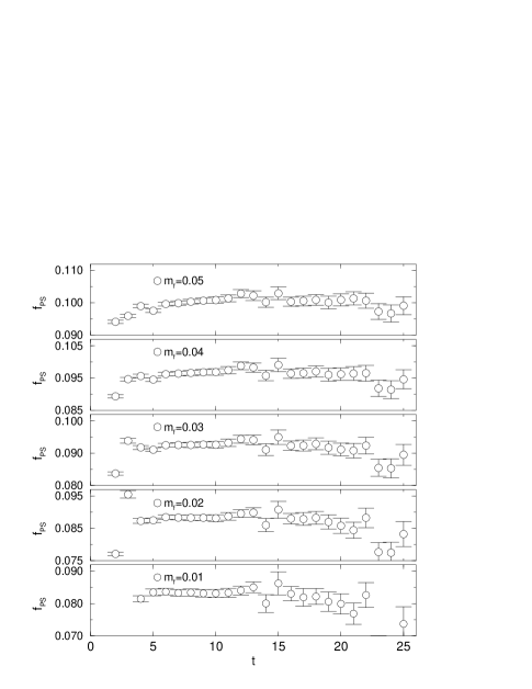
Figure 14: Same plot as Fig. 13 but for DBW2 $\beta=1.04$. The fitting range $12\leq t\leq 19$ was used to extract $f_{\rm PS}^{(1)}$ for this case.

Figure 15: Renormalization factor $Z_{A}$ as a function of $m_{f}+m_{res}$ for DBW2 $\beta=1.22$.

Figure 21: Renormalization factors $Z_{q}^{-2}Z_{VV+AA,\ VV-AA}$ as a function of $m_{f}+m_{\rm res}$ for several fixed values of $p_{\rm latt}^{2}$, for each of which a linear fit is drawn.

Figure 26: The quantity $\left\langle\overline{\rm PS}\left|Q^{(\Delta S=2)}\right|\rm PS\right\rangle$ plotted as a function of $m_{\rm PS}^{2}$ [${\rm GeV}^{2}$] for DBW2 $\beta=1.22$ (left) and $\beta=1.04$ (right). The curves are fits to Eq. 45.

Figure 31: B-parameters for ${\cal O}_{VV+AA}$ (circle), ${\cal O}_{VV-AA}$ (square), ${\cal O}_{SS-PP}$ (diamond), ${\cal O}_{SS+PP}$ (triangle) and ${\cal O}_{TT}$ (left-triangle) for DBW2 $\beta=1.04$ as a function of $m_{f}$.

References

- (1) G. Buchalla, A. J. Buras, and M. E. Lautenbacher, Rev. Mod. Phys. 68, 1125 (1996), eprint hep-ph/9512380.
- (2) Y. Kuramashi, Nucl. Phys. Proc. Suppl. 83, 24 (2000), eprint hep-lat/9910032.
- (3) L. Lellouch, Nucl. Phys. Proc. Suppl. 94, 142 (2001), eprint hep-lat/0011088.
- (4) G. Martinelli, Nucl. Phys. Proc. Suppl. 106, 98 (2002), eprint hep-lat/0112011.
- (5) N. Ishizuka, Nucl. Phys. Proc. Suppl. 119, 84 (2003), eprint hep-lat/0209108.
- (6) D. Becirevic, Nucl. Phys. Proc. Suppl. 129, 34 (2004).
- (7) M. Wingate, Nucl. Phys. Proc. Suppl. 140, 68 (2005), eprint hep-lat/0410008.
- (8) S. Aoki et al. (JLQCD), Phys. Rev. D60, 034511 (1999), eprint hep-lat/9901018.
- (9) L. Lellouch and C. J. D. Lin (UKQCD), Nucl. Phys. Proc. Suppl. 73, 312 (1999), eprint hep-lat/9809142.
- (10) S. Aoki et al. (JLQCD), Phys. Rev. Lett. 80, 5271 (1998), eprint hep-lat/9710073.
- (11) P. Dimopoulos, J. Heitger, C. Pena, S. Sint, and A. Vladikas (ALPHA), Nucl. Phys. Proc. Suppl. 129, 308 (2004), eprint hep-lat/0309134.
- (12) C. T. H. Davies et al. (HPQCD), Phys. Rev. Lett. 92, 022001 (2004), eprint hep-lat/0304004.
- (13) C. Aubin et al., Phys. Rev. D70, 094505 (2004), eprint hep-lat/0402030.
- (14) H. Neuberger, Phys. Lett. B417, 141 (1998), eprint hep-lat/9707022.
- (15) D. B. Kaplan, Phys. Lett. B288, 342 (1992), eprint hep-lat/9206013.
- (16) Y. Shamir, Nucl. Phys. B406, 90 (1993), eprint hep-lat/9303005.
- (17) V. Furman and Y. Shamir, Nucl. Phys. B439, 54 (1995), eprint hep-lat/9405004.
- (18) H. Neuberger, Phys. Rev. Lett. 81, 4060 (1998), eprint hep-lat/9806025.
- (19) R. G. Edwards, U. M. Heller, and R. Narayanan, Nucl. Phys. B540, 457 (1999), eprint hep-lat/9807017.
- (20) T. Blum et al., Phys. Rev. D66, 014504 (2002), eprint hep-lat/0102005.
- (21) T. Blum et al. (RBC), Phys. Rev. D68, 114506 (2003), eprint hep-lat/0110075.
- (22) T. Takaishi, Phys. Rev. D54, 1050 (1996).
- (23) P. de Forcrand et al. (QCD-TARO), Nucl. Phys. B577, 263 (2000), eprint hep-lat/9911033.
- (24) T. Blum and A. Soni, Phys. Rev. D56, 174 (1997), eprint hep-lat/9611030.
- (25) T. Blum and A. Soni, Phys. Rev. Lett. 79, 3595 (1997), eprint hep-lat/9706023.
- (26) A. Ali Khan et al. (CP-PACS), Phys. Rev. D63, 114504 (2001), eprint arXiv:hep-lat/0007014.
- (27) T. Blum et al., Phys. Rev. D69, 074502 (2004), eprint hep-lat/0007038.
- (28) R. D. Mawhinney, Nucl. Phys. Proc. Suppl. 83-84, 57 (2000), eprint hep-lat/0001032.
- (29) Y. Aoki et al., Phys. Rev. D69, 074504 (2004), eprint hep-lat/0211023.
- (30) A. Ali Khan et al. (CP-PACS), Phys. Rev. D64, 114506 (2001), eprint hep-lat/0105020.
- (31) Y. Aoki et al. (2004), eprint hep-lat/0411006.
- (32) N. Garron, L. Giusti, C. Hoelbling, L. Lellouch, and C. Rebbi, Phys. Rev. Lett. 92, 042001 (2004), eprint hep-ph/0306295.
- (33) T. DeGrand (MILC), Phys. Rev. D69, 014504 (2004), eprint hep-lat/0309026.
- (34) J. Noaki (RBC), Nucl. Phys. Proc. Suppl. 119, 362 (2003), eprint hep-lat/0211013.
- (35) J. Noaki (RBC), Nucl. Phys. Proc. Suppl. 129, 269 (2004), eprint hep-lat/0309175.
- (36) Y. Iwasaki UTHEP-118.
- (37) Y. Iwasaki, Nucl. Phys. B258, 141 (1985).
- (38) M. Guagnelli, R. Sommer, and H. Wittig (ALPHA), Nucl. Phys. B535, 389 (1998), eprint hep-lat/9806005.
- (39) K. Hashimoto and T. Izubuchi (RBC), Nucl. Phys. Proc. Suppl. 140, 341 (2005), eprint hep-lat/0409101.
- (40) T. DeGrand, A. Hasenfratz, and T. G. Kovacs, Nucl. Phys. B520, 301 (1998), eprint hep-lat/9711032.
- (41) A. Morel, J. Phys. (France) 48, 1111 (1987).
- (42) S. R. Sharpe, Phys. Rev. D46, 3146 (1992), eprint hep-lat/9205020.
- (43) C. W. Bernard and M. F. L. Golterman, Phys. Rev. D46, 853 (1992), eprint hep-lat/9204007.
- (44) P. Lacock and C. Michael (UKQCD), Phys. Rev. D52, 5213 (1995), eprint hep-lat/9506009.
- (45) G. Martinelli, C. Pittori, C. T. Sachrajda, M. Testa, and A. Vladikas, Nucl. Phys. B445, 81 (1995), eprint hep-lat/9411010.
- (46) C. Dawson, Nucl. Phys. Proc. Suppl. 83-84, 854 (2000), eprint hep-lat/9909107.
- (47) C. Dawson (RBC), Nucl. Phys. Proc. Suppl. 94, 613 (2001), eprint hep-lat/0011036.
- (48) M. Ciuchini, E. Franco, G. Martinelli, L. Reina, and L. Silvestrini, Z. Phys. C68, 239 (1995), eprint hep-ph/9501265.
- (49) M. Ciuchini et al., Nucl. Phys. B523, 501 (1998), eprint hep-ph/9711402.
- (50) S. Capitani, M. Luscher, R. Sommer, and H. Wittig (ALPHA), Nucl. Phys. B544, 669 (1999), eprint hep-lat/9810063.
- (51) S. Aoki, T. Izubuchi, Y. Kuramashi, and Y. Taniguchi, Phys. Rev. D67, 094502 (2003), eprint hep-lat/0206013.
- (52) M. F. L. Golterman and K.-C. Leung, Phys. Rev. D57, 5703 (1998), eprint hep-lat/9711033.
- (53) Y. G. Zhestkov UMI-30-28611.
- (54) M. Crisafulli et al., Phys. Lett. B369, 325 (1996), eprint hep-lat/9509029.
- (55) R. Gupta, T. Bhattacharya, and S. R. Sharpe, Phys. Rev. D55, 4036 (1997), eprint hep-lat/9611023.
- (56) S. Aoki et al. (JLQCD), Phys. Rev. Lett. 81, 1778 (1998), eprint hep-lat/9705035.
- (57) L. Conti et al., Phys. Lett. B421, 273 (1998), eprint hep-lat/9711053.
- (58) D. Becirevic, P. Boucaud, V. Gimenez, V. Lubicz, and M. Papinutto, Eur. Phys. J. C37, 315 (2004), eprint hep-lat/0407004.
- (59) M. Golterman and Y. Shamir, Phys. Rev. D71, 034502 (2005), eprint hep-lat/0411007.
- (60) M. Golterman and Y. Shamir, Phys. Rev. D68, 074501 (2003), eprint hep-lat/0306002.