Interactions of confining strings in SU(3) gluodynamics

Abstract

We study the interaction energy of the confining strings in the static rectangular tetraquark system in SU(3) gluodynamics. Using a two-state approximation we calculate the energy eigenvalues and corresponding eigenvectors of string states of different geometry. The interactions are studied both for the co-aligned and for the counter-aligned parallel strings as the functions of positions of the tetraquark constituents. We formulate a simple soap-film model and show that with a good accuracy the string interaction energy corresponding to the ground state of the tetraquark system can be described by this soap-film model.

I Introduction and Motivation

The complicated phenomenology of the strong interactions at low energies – such as the spectrum of mesons and baryons as well as the properties of their resonances – is determined by the forces between hadronic constituents, quarks and antiquarks. These forces are dependent on spin orientations, relative velocities and distances between the quarks and (anti-)quarks in the bound states ref:Reviews:QCDforces ; ref:Reviews:correlators . The major role in the QCD spectrum is played by the quark confinement which implies that the quarks are not observed as asymptotic states.

In SU(3) gluodynamics the confinement manifests itself as a strong ($\approx 1\mbox{GeV}/\mbox{fm}$) attractive force between an external quark and an anti-quark as they get separated by large enough distances. It is believed that this force is a result of a formation of a flux tube, or a QCD string, between the external color charges. Since the QCD string has a constant energy per unit length the confining force is asymptotically separation-independent.

In the real QCD the confining force is screened by pairs of quarks and anti-quarks which emerge from the vacuum and break an exceedingly long QCD string. Still the confining force caused by the QCD strings plays a crucial role in the structure of hadronic bound states and their resonances when these systems have sufficiently large spatial size. It is very plausible that the hadron structure is influenced not only by the interaction between the quarks themselves (i.e., between the ends of the QCD string) but also by the interaction between the segments of the QCD string(s) with each other. The role of the QCD string interactions is the main subject of this article. Since the origin of the string and, consequently, the essence of confinement, is encoded in the gluonic degrees of freedom, we restrict ourselves to the quenched QCD case.

The three-quark (baryon) state represents a simplest non-trivial case of the inter-string interactions. In the baryon there are two possible geometries of the QCD string connecting three quarks: the $\Delta$–like geometry which connects the quarks pairwise and the $Y$–like geometry which connects quarks by three segments of the string with a junction in a middle. Lattice study of the baryon static potential revealed that the potential agrees with the dominance of the two-body interaction at small interquark separations Takahashi:2002bw ; Alexandrou:2002sn ; Bornyakov:2004uv . This result is natural from the point of view point of the asymptotic freedom which predicts that at short distances the interquark interactions are reduced to the two-body interquark forces.

The $Y$-shape of the QCD string is difficult to observe at short distances due to the dominance of the Coulomb potentials . However, as the interquark separations get larger, the $Y$-ansatz behavior prevails the two-body interactions Takahashi:2002bw ; Alexandrou:2002sn ; Bornyakov:2004uv . The $Y$–type profile of the QCD string was also observed at large inter-quark separations in quenched and unquenched lattice QCD in Refs. ref:profile:DIK ; Bornyakov:2004uv where Abelian projection was used as a useful tool. In Ref. Bissey:2005sk the $Y$–type profile was observed in unquenched lattice QCD with the help of gauge invariant operators.

The $Y$-geometry of the flux tube profile in baryon-like configuration of quarks is consistent with the prediction ref:Y-DGL of the dual superconductivity scenario ref:DualSuperconductor , which is assumed to work in the infrared region (for a review see Refs. ref:Reviews ). The field correlator method also predicts the $Y$-geometry of the strings in the baryon Kuzmenko:2003ck .

In order to investigate the interaction between QCD strings it is convenient to consider a geometry with two long disconnected segments of the string. This corresponds to a generalization of the baryonic system to a system consisting of four or more (anti)quarks. In this case, the interactions between the QCD strings can be deduced from the interquark potentials. The multi-quark potentials were intensively studied on the lattice ref:Ydominance ; ref:Helsinki ; ref:suganuma:4Q ; ref:alexandrou:4Q ; ref:suganuma:5Q ; ref:alexandrou:5Q . In the simplest case of the SU(2) gauge theory, the chromoelectric string does not have a directional dependence since quarks and anti-quarks in this theory are indistinguishable from each other. A numerical study of energies in the four-quark systems shown that the interaction, or binding, energy is nonzero in the general case ref:Helsinki . It was found that if the four quarks are partitioned into a colorless two-meson state with basic states degenerate (or, almost degenerate) in energy, then the interaction energy of the system is strongly enhanced. It was thus shown that the energies of the four-quark states cannot be simply represented as a sum in terms of two-quark potentials. These features indicate that the mutual interaction of the chromoelectric strings can not be ignored in the SU(2) four-quark systems.

In the SU(3) gluodynamics investigation of the interaction energy of the tetraquark system with two co-aligned mesons has shown ref:suganuma:4Q ; ref:alexandrou:4Q that the strings form a joint profile with two $Y$-type junctions for small enough separations between the mesons.

The two-meson interactions were also studied analytically in the dual superconductor model in the SU(2), Ref. ref:Suzuki:intermeson and SU(3), Ref. ref:Y-DGL ; ref:SU3:string:interaction cases, as well as in the gauge–invariant field–strength cumulant approach ref:Reviews:correlators ; ref:Simonov:Shevchenko .

Apart from purely theoretical interest in investigation of the inter-string interactions (potentially applicable to physical systems) there is a direct experimental motivation to study the 4Q systems in particular. Presently, candidates for a $4Q$ state include the $X$(3872) resonance ref:X as discussed in Ref. ref:X:theory , and $D_{s}$(2317) state ref:Ds . The knowledge of the flux tube structure in the four quark systems seems to be important also in hadron scattering reactions since these reactions may also involve a rearrangement of the confining strings.

In this paper we study the interactions of the QCD strings in the system consisting of two quarks and two anti-quarks. The general considerations concerning the interactions of the two (segments of) confining strings are discussed in Section II. In order to calculate the interaction energy we diagonalize the QCD Hamiltonian in the basis of the two lowest energy states. As a guiding example, the calculation of matrix elements of a Hamiltonian is done analytically in Section III in a soap-film approximation which resembles the strong coupling expansion in the lattice gluodynamics. This calculation – which is of a qualitative nature – is then compared with the results of the lattice simulations of SU(3) gluodynamics discussed in Section IV. Our conclusions are summarized in Section V. The technical details of the numerical procedures as well as principal output of simulations are presented in Appendices.

II Interactions between QCD strings

The QCD strings have finite width but if they are long enough they can be considered as line-like objects connecting quarks or/and anti-quarks in three spatial dimensions. In a meson system the strings carry the chromoelectric flux which originates at a quark and is absorbed at an anti-quark. The interaction between the strings can be studied numerically with the help of the correlator of two large Wilson loops separated by a large enough distance. The correlator must be appropriately normalized by the expectation values of the individual Wilson loops, in order to subtract the energies of the infinitely separated quark–antiquark pairs. The interaction energy $E_{int}(d,r)$ is then defined as

$$E_{\mathrm{int}}(d,r)=-\lim_{t\to\infty}\frac{1}{t}\log\frac{\langle W_{r\times t}(0)\,W_{r\times t}(d)\rangle}{\langle W_{r\times t}(0)\rangle\,\langle W_{r\times t}(d)\rangle}\,,$$ (1)

where $W_{r\times t}$ is the rectangular Wilson loop of size $r\times t$, $d$ is the distance between two parallel meson systems. The Wilson loop $W_{r\times t}$ describes the evolution of the quark–antiquark pair separated by the distance $r$ from time $t_{0}=0$ to time $t_{1}=t$.

In Eq. (1) the time extension $t$ of the Wilson loops should be taken infinite. In order to study string interaction contribution into the full interaction energy one should also take $r$ to be large in order to avoid effects of the short range Coulomb interaction between static quarks. In the real lattice simulations the above requirements are difficult to comply with.

II.1 Flip-flop picture

The important difference between the “ideal” strings discussed above and the “real” strings in lattice simulations is the fact that a lattice string has a finite length $r$ and is evolved over a finite Euclidean time $t$. The constraints on $r$ and $t$ are due to the finiteness of the lattice volume. As a result of this finiteness, there are some effects which make the interpretation and realization of the Eq. (1) difficult.

The finite $t$ implies the influence of higher excitations (this effect is common to all lattice studies). We will address the question of the $t$–dependence of our numerical results in Appendix B.1 where we show that the results are rather stable against this kind of systematic errors.

If the distance $d$ is not large enough then the (anti)quark of one quark-antiquark pair is interacting with the one of the other quark-antiquark pair  providing an unwanted contribution to the interaction energy $E_{\mathrm{int}}$. As a smearing technique we are using the hypercubic blocking (HYP) to improve the signal to noise ratio for our observables, also decreases effects of the short range inter quark interaction. As it was shown in Ref. hyp2 , the perturbative interaction – which dominates the interactions of quarks at small separations – is suppressed by the HYP blocking. An interested reader can find the details of the HYP blocking in Appendix A.2.

The effect of finite length $r$ is seen in a string rearrangement which is also known as the ”flip-flop” effect discussed in the context of SU(2), Ref. ref:Helsinki , and SU(3), Ref. ref:suganuma:4Q , lattice gauge theories. The flip-flop is a string rearrangement process which happens as one changes the positions of the ends of the strings (quarks). The rearrangement is caused by a requirement for the strings to be in the ground state, i.e. in a state with lowest possible (for given boundary conditions) value of energy. As we will see later this is basically the same as the requirement for the string configuration to have a shortest possible length.

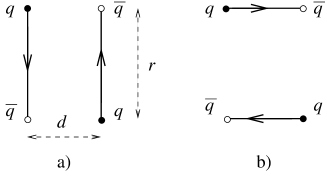
Figure 1: A schematic illustration of the flip-flop picture: (a) the longitudinal and (b) the transverse string configurations.

The rearrangement is illustrated in Fig. 1 for the simplest case of two parallel strings with the same length and opposite orientations. This string configuration is called below the “longitudinal” configuration. The two quarks and two antiquarks shown in Fig. 1(a) can also be connected by strings in another way shown schematically in Fig. 1(b). Below we call the latter “transverse” configuration. Let us keep the size $r$ of the pair fixed and decrease the separation $d$. When $d$ becomes smaller than some critical value $d_{c}$ the energy of the transverse configuration becomes smaller than the one for the longitudinal configuration. It is energetically favorable for the strings to realign at this point. Having neglected an interaction between the segments of the string, we can estimate an energy of the string configuration as $E\approx\sigma L$, where $L$ is a total length of the string configuration, and $\sigma$ is the universal string tension. Obviously, due to a simple geometry of the string configuration shown in Fig. 1, the distances $d_{c}$ and $r$ are approximately equal in this particular example. However, in other systems the competitive configurations can be more complicated, like the one shown in Fig. 2 for the case of equally oriented strings. The critical separation in this case is estimated to be $d_{c}\simeq r/\sqrt{3}$.

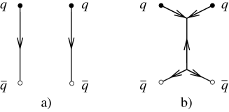
Figure 2: The string configurations for the quark pairs with the same orientation: (a) the longitudinal configuration; (b) The transverse configuration with two string junctions. The minimal length corresponding to the case (b) is $L_{b}=r+\sqrt{3}d$.

If one treats the string configuration classically, the string re-alignment indicates existence at the flip-flop point $d=d_{c}$ of (at least) two degenerate energy minima in the space of the string configurations. On the quantum level, the degeneracy leads to the level splitting effect, as it is well known from the quantum mechanics. The level splitting is caused by the tunneling transitions between the wells of potential energy. Therefore one expects that the “transverse” and the “longitudinal” string states are mixed with each other due to the tunneling transitions and, consequently, the degeneracy is taken away. Technically, the tunneling transitions lead to an appearance of the non-diagonal matrix elements of the Hamiltonian in the basis of the original states (i.e., the states corresponding to the far-separated ”unperturbed” individual wells). To get the correct energy states one needs to diagonalize the Hamiltonian taking into account the tunneling transitions. The true ground state of the string in a tetraquark is a weighted mix of all ”unperturbed” states of this system. In the two– and three-quark systems a similar investigation was performed, respectively, in Refs. ref:Morningstar and ref:gluonic:excitation in order to investigate gluonic excitations.

In order to treat the degeneracy of the ground state exactly one needs to consider not only the ground state itself but also one should know all the states of the system. However, the higher is the state the lower is its mixing with the ground state. Therefore, one usually considers the two-state approximation, which takes into account only the ground state and the next energy state of the string system. Technically, this approach corresponds to the diagonalization of the Hamiltonian in the two dimensional subspace of the states.

II.2 Two-level Approximation

We can construct (”prepare”) an operator to study the particular configuration of the quarks and anti-quarks by connecting the corresponding sets of points in a three-dimensional time-slice by gauge transporters. These transporters, called sometimes as ”Schwinger lines”, are the open Wilson lines in the fundamental representation of the gauge group. Such a set of lines transforms under gauge transformations as a set of quarks and anti-quarks. The better is the overlap of this operator with the real multiquark ground state (determined by the QCD dynamics) the smaller are effects of higher excitations. In order to improve this overlap we use the APE smeared gauge transporters, see Appendix A.1 for details.

We consider the configurations of the Wilson lines shown in Figures 1 and 2. The corresponding states define a two dimensional subspace of the state space discussed in the previous Subsection. The explicit definition of the basis of the states depends on positions of quarks and anti-quarks. We consider two simple geometries: co-aligned (Fig.2) and oppositely aligned (Fig.1) parallel strings of the same length, and we present the exact expressions concurrently where the relative orientation makes a difference.

The initial states of our basis – corresponding to the classical string configurations – are shown in Table 1. The oriented lines mean the gauge transporters, the closed contour is the Wilson loop, and $N_{c}=3$ is the number of colors used to normalize the initial states. We refer to these basis states as $|A\rangle$ and $|B\rangle$ regardless of the orientation. Although the states are normalized, $\langle A|A\rangle=\langle B|B\rangle=1$, they are not, in general, orthogonal to each other,

$$g\equiv\langle A|B\rangle\neq 0\,.$$ (2)

The basis states overlap $g$ is proportional to the spatial Wilson loop and also shown in Table 1.

	Opposite orientation	Same orientation
$|A\rangle$	$N^{-1}_{c}\begin{array}[]{l}\includegraphics[width=51.21495pt]{eps/def_a.eps}\end{array}|0\rangle$	$N^{-1}_{c}\begin{array}[]{l}\includegraphics[width=51.21495pt]{eps/def_c.eps}\end{array}|0\rangle$
$|B\rangle$	$N^{-1}_{c}\begin{array}[]{l}\includegraphics[width=51.21495pt]{eps/def_b.eps}\end{array}|0\rangle$	$N^{-1/2}_{c}\begin{array}[]{l}\includegraphics[width=51.21495pt]{eps/def_d.eps}\end{array}|0\rangle$
$\langle B|A\rangle$	$N^{-1}_{c}\langle 0|\begin{array}[]{l}\includegraphics[width=51.21495pt]{eps/gab.eps}\end{array}|0\rangle$	$N^{-1/2}_{c}\langle 0|\begin{array}[]{l}\includegraphics[width=51.21495pt]{eps/gcd.eps}\end{array}|0\rangle$

Table 1: The graphical definition of the states from the initial basis and of their overlap.

Let us consider the diagonalization of the Hamiltonian $\hat{H}$ in the space $|A\rangle\oplus|B\rangle$. To this end one can first diagonalize the Euclidean time evolution operator

$$\hat{S}(t)=\exp(-\hat{H}t)\,,$$ (3)

the matrix elements of which can be calculated in lattice simulations. Despite the operator identity (3) is not correct in the finite basis, $S_{ab}\neq\exp(-H_{ab}t)$, one expects that only the lowest energy states contribute to the evolution operator matrix elements for large enough evolution time $t$. We will see that the $t$-dependence of the energy levels, defined via evolution operator eigenstates, has a form of $1/t$ corrections and, consequently, can be neglected for large enough $t$.

The main observables calculated in our numerical simulations are the $S$ matrix elements:

$${\mathbf{S}}(t)=\left(\begin{array}[]{rr}\langle A|e^{-Ht}|A\rangle&\langle B|e^{-Ht}|A\rangle\\ \langle A|e^{-Ht}|B\rangle&\langle B|e^{-Ht}|B\rangle\end{array}\right)\,.$$ (4)

They are expressed as the Wilson loops correlators which for the case of the oppositely aligned strings can graphically be represented as follows:

$${\mathbf{S}}(t)= \langle 0|\left(\begin{array}[]{rr}\begin{array}[]{l}\includegraphics[height=51.21495pt]{eps/aa.eps}\end{array}&N^{-1}_{c}\begin{array}[]{l}\includegraphics[height=51.21495pt]{eps/ab.eps}\end{array}\\ N^{-1}_{c}\begin{array}[]{l}\includegraphics[height=51.21495pt]{eps/ba.eps}\end{array}&\begin{array}[]{l}\includegraphics[height=51.21495pt]{eps/bb.eps}\end{array}\end{array}\right)|0\rangle\,.$$ (11)

For co-aligned strings the graphical representation is a bit more complicated:

$${\mathbf{S}}(t)= \langle 0|\left(\begin{array}[]{rr}\begin{array}[]{l}\includegraphics[height=51.21495pt]{eps/cc.eps}\end{array}&N^{-1/2}_{c}\begin{array}[]{l}\includegraphics[height=51.21495pt]{eps/cd.eps}\end{array}\\ N^{-1/2}_{c}\begin{array}[]{l}\includegraphics[height=51.21495pt]{eps/dc.eps}\end{array}&\begin{array}[]{l}\includegraphics[height=51.21495pt]{eps/dd.eps}\end{array}\end{array}\right)|0\rangle\,.$$ (18)

The problem to find eigenfunctions and eigenvalues of the matrix $S$

$$\hat{S}(t)|E\rangle=\exp(-Et)|E\rangle\,,$$ (19)

can be reformulated as a generalized eigenproblem in terms of the matrix elements,

$$S_{ab}(t)h_{b}=\lambda(t)T_{ab}h_{b}\,,$$ (20)

where $a,b\in\{A,B\}$ and $|E\rangle=h_{A}|A\rangle+h_{B}|B\rangle$. The matrix ${\mathbf{T}}$ in the right-hand side of Eq. (20) is nothing but the overlap of the basis states, discussed above,

$${\mathbf{T}}=\left(\begin{array}[]{rr}1&g\\ g&1\end{array}\right)\,.$$ (21)

Equation (20) together with the normalization condition

$$\langle E|E\rangle=h_{A}^{2}+h_{B}^{2}+2gh_{A}h_{B}=1$$ (22)

defines two eigenstates $|E_{0,1}\rangle$ of the evolution operator (and, with all precautions, of the Hamiltonian). These eigenstates correspond to the energies

$$E_{0,1}=-\frac{\ln(\lambda_{0,1})}{t}\,.$$ (23)

In order to solve the eigenproblem one should know all the matrix elements $S_{ab}(t)$. To understand the qualitative properties of the eigenvalues we perform an analytical calculation in the soap-film approximation in the next Section.

Note that we call the energy $E_{0}$ as the ground state energy while the energy $E_{1}$ is refereed to as the excited energy. This standard terminology – the ground state corresponds to the lowest energy while the excited state to the higher one – should not be taken literally. Indeed, the states correspond to different string configurations in the sense of geometry (like in Figures 1 and 2), and they most probably should not be interpreted as the excited (i.e., vibrational) modes of one of (the segments of) the strings. Such excited modes were studied in the case of a single QCD string in a static meson ref:Morningstar , and in a case of the simply-connected $Y$-shaped string segments in the case of a static baryon ref:gluonic:excitation . In the sense of such excited mode both energies $E_{0}$ and $E_{1}$ correspond to the ground states of the particular string configurations visualized schematically in Figures 1 and 2.

III Soap-film approximation

	Opposite orientation	Same orientation
$S_{AA}$	$~{}~{}~{}\begin{array}[]{l}\includegraphics[height=51.21495pt]{eps/saa.10.eps}\end{array}~{}+~{}\displaystyle{\frac{1}{N^{2}_{c}}}\begin{array}[]{l}\includegraphics[height=51.21495pt]{eps/saa.20.eps}\end{array}$	$~{}~{}~{}\begin{array}[]{l}\includegraphics[height=51.21495pt]{eps/scc.10.eps}\end{array}~{}+~{}\displaystyle{\frac{1}{N_{c}}}\begin{array}[]{l}\includegraphics[height=51.21495pt]{eps/scc.20.eps}\end{array}$
$S_{BB}$	$~{}~{}~{}\begin{array}[]{l}\includegraphics[height=51.21495pt]{eps/sbb.10.eps}\end{array}~{}+~{}\displaystyle{\frac{1}{N^{2}_{c}}}\begin{array}[]{l}\includegraphics[height=51.21495pt]{eps/sbb.20.eps}\end{array}$	$~{}~{}~{}\begin{array}[]{l}\includegraphics[height=51.21495pt]{eps/sdd.10.eps}\end{array}~{}+~{}\displaystyle{\frac{1}{N_{c}}}\begin{array}[]{l}\includegraphics[height=51.21495pt]{eps/sdd.20.eps}\end{array}$
$S_{AB}$	$~{}~{}~{}\displaystyle{\frac{1}{N_{c}}}\left(\begin{array}[]{l}\includegraphics[height=51.21495pt]{eps/sab.10.eps}\end{array}~{}+~{}\begin{array}[]{l}\includegraphics[height=51.21495pt]{eps/sab.20.eps}\end{array}\right)$	$~{}~{}~{}\displaystyle{\frac{1}{\sqrt{N_{c}}}}\left(\begin{array}[]{l}\includegraphics[height=51.21495pt]{eps/scd.10.eps}\end{array}~{}+~{}\begin{array}[]{l}\includegraphics[height=51.21495pt]{eps/scd.20.eps}\end{array}\right)$

Table 2: The soap-film expansion of the evolution matrix elements ($S_{BA}=S_{AB}$).

In the soap-film approximation we evaluate the average of the Wilson loops taking into account only the area contributions

$$\langle 0|W_{1}\dots W_{n}|0\rangle\Longrightarrow\sum_{i}k_{i}\exp(-\sigma S_{i}),$$ (24)

where the sum is taken over all topologically distinct and locally minimal surfaces with the area $S_{i}$ which are spanned on a given set of oriented contours. The integer pre-factors $k_{i}$ count the number of string configurations which can be spanned on the given set of loops. Finally, $\sigma$ is the universal string tension.

In general, Eq. (24) can be justified either in the strong coupling regime (discussed in Ref. ref:alexandrou:4Q for the multi-quark interaction) or in the infrared region, where the perimeter-like contributions to the Wilson loops can be neglected. Moreover, the soap-film expansion – applied in the infrared region – coincides with the field-strength correlator expansion performed in Ref. ref:Simonov:Shevchenko to study interactions of the Wilson loops in the Gaussian approximation.

The essential point is that in Eq. (24) we neglect the string fluctuations, the contribution of which is small compared with the leading area term. Note that in the discussed approximation (24) any local string interactions (e.g. via exchange of a particle) are neglected. On the other hand, the effect of re-alignment is still encoded in Eq. (24), therefore this representation ideally suits our needs as a simple theoretical model.

The expansion of the matrix elements (11),(18) is shown in Table 2. Overall normalization of the matrix elements can easily be obtained from the normalization of the basis states. The color factors $1/N_{c}$ and $1/N^{2}_{c}$ in the non-planar contributions to the diagonal matrix elements appears in the strong coupling expansion and in the field-strength approach ref:Simonov:Shevchenko .

Decomposing the surfaces into the spatial and the time-like faces,

$$\exp(-\sigma S)=\prod_{faces}\exp(-\sigma S_{i})\,,$$ (25)

and identifying the spatial contributions with the basis states overlap $g$, one derives

$${\mathbf{S}}(t)=f_{r}\left(\begin{array}[]{rr}1&g\\ g&g^{2}\end{array}\right)+f_{d}\left(\begin{array}[]{rr}g^{2}&g\\ g&1\end{array}\right)\,,$$ (26)

where

$$f_{r}=\exp(-2\sigma rt)\,,$$ (27)

and

$$f_{d}=\left\{\begin{array}[]{lr}\exp(-2\sigma dt)&\textrm{opposite orientation}\\ \exp(-\sigma(\sqrt{3}d+r)t)&\textrm{same orientation}\end{array}\right.\,.$$ (28)

The characteristic equation corresponding to Eq. (20),

$$\det({\mathbf{S}}(t)-\lambda{\mathbf{T}})=0\,,$$ (29)

where ${\mathbf{T}}$ is defined in (21), has the following roots

$$\lambda_{0,1}~{}=~{}\frac{1}{2}(f_{d}+f_{r}\pm\sqrt{(f_{d}-f_{r})^{2}+4g^{2}f_{d}f_{r}})\,.$$ (30)

Finally, the energy levels are obtained with the help of Eq. (23).

We are interested in the two regions of the parameter space: (i) the region near the flip-flop point $r=d$ and (ii) the “interaction” region corresponding to the two relatively long strings placed near each other, $d\ll r$.

• At the flip-flop point $f_{r}=f_{d}=f$. Then Eq.(30) becomes

  $$\lambda_{0,1}|_{d=d_{c}}=f(1\pm g)\,,$$ (31)

  giving the levels splitting (valid for both string orientations)

  $$(E_{1}-E_{0})|_{d=d_{c}}=\frac{1}{t}\ln\frac{1+g}{1-g}=\frac{2g+o(g)}{t}\,.$$ (32)

  Thus the level splitting is just a finite $t$ effect in the case when the basis of the Hamiltonian eigenstates is truncated (the true Hamiltonian eigenvalues do not depend on $t$ in the full basis).

• At the interaction region the energy splitting can be obtained by an expansion of the square root in Eq.(30) in powers of $f_{r}/f_{d}$,

  $$\lambda_{0} = f_{d}\{1+f_{r}/f_{d}\cdot g^{2}+o(f_{r}/f_{d})\}$$ (33a)

  $$\lambda_{1} = f_{r}\{1-g^{2}-f_{r}/f_{d}\cdot g^{2}(1-g^{2})+o((f_{r}/f_{d})^{2})\}\,.$$ (33b)

  Then the leading contribution to the energy levels takes the following form (the orientation is explicitly indicated),

  $$E_{0}|_{d\to 0} = \left\{\begin{array}[]{ll}2\sigma d&\textrm{opposite}\\ \sigma(\sqrt{3}d+r)&\textrm{same}\end{array}\right.$$ (34c)

  $$E_{1}|_{d\to 0} = 2\sigma r-\frac{\ln(1-g^{2})}{t}=2\sigma r+\frac{g^{2}+o(g^{2})}{t}\,,$$ (34d)

  leading just to the “classical” string configurations up to the $1/t$ corrections. In this case the interaction is absent as it was expected.

An exact (unexpanded) expressions for the eigenvalues as functions of the parameters $d$ and $r$ are too bulky we skip their functional forms here. However, we present the soap-film results in the graphical form in the next Section in order to compare them with the lattice data.

For the comparison of the lattice data and the soap-film predictions, the latter should be improved to cover the small $d$ and $r$ regions in a parameter space, for which the Wilson loops are not saturated by area law. A possible way to do this systematically is to make in Eq. (25) a substitution of single Wilson loop averages for time-like faces (which is supposed to be an area-law behavior in the soap-film formalism) by the expression

$$\exp(-\sigma S_{i})\Rightarrow\langle W_{i}\rangle=\exp(-V(r_{i})t)$$ (35)

where $i$ runs over all plain time-like faces of size $r_{i}\times t$, bounded by rectangular Wilson loop and $\langle W\rangle$ is related to the static quark-antiquark potential $V(r)$. In fact we already performed this trick when we used for the spatial faces the overlap $g(r,d)$ instead of the area-law expression which would originate from the soap-film formalism.

The equations (27),(28) now look as:

$$f_{r}=\exp(-2V(r)t),$$ (36)

and

$$f_{d}=\left\{\begin{array}[]{ll}\exp(-2V(d)t)&\textrm{opposite orientation}\\ \exp(-(4V(d/\sqrt{3})+V(r-d/\sqrt{3}))t)&\textrm{same orientation}\end{array}\right.\,.$$ (37)

All other expressions remain unchanged. In order to perform the improvement we evaluate numerically the static potential $V(r)$ and the overlap function $g(r,d)$. Below we use the improved soap-film formulation instead of the naive area-law expansion.

IV Lattice Data

Figure 3: The energy eigenvalues $E_{0,1}(r,d)$ as the functions of the string separation $d$ at the fixed string length $r=0.84$ fm. The left (right) plot corresponds to the oppositely aligned (co-aligned) strings. The points corresponds to the numerical data obtained in simulations while the lines are the soap-film predictions. The statistical errors of both data points are of the order of the symbol size. The error in estimation of the soap film prediction is of the same magnitude. Note that in all our numerical results the perturbative contributions are suppressed by the HYP procedure

Ground state                                                              Excited state

Figure 4: The difference between $\delta E=E-E_{\mathrm{soap}}$ the measured energy levels and the prediction of the soap-film approximation for the oppositely aligned strings of the length $r=0.84$ fm. The points represent $\delta E$ while the band represent the statistical errors of soap-film prediction. Note the MeV scale of vertical axis compared to the GeV scale of interaction energy in Fig. 3.

Ground state                                                              Excited state

Figure 5: The same as in Fig. 5 but for the likewise oriented strings.

In order to obtain energy eigenvalues and eigenvectors one needs to know the evolution matrix elements $S_{ab}$ given in Eq.(11),(18), the overlap of the basis states $g(r,d)$ and the static potential $V(r)$. Since all mentioned observables are expressed in terms of the Wilson loops correlators, we perform a lattice computation which is straightforward. The details of numerical setup and computation details are given in Appendix A.

The analysis is performed similarly to the analytical case of the soap-film expansion presented in the previous Section. The energy levels of oppositely aligned and co-aligned strings are provided as functions of parameters $r,d$ in, respectively, Tables 5 and 6 of Appendix B.

In Fig. 3 we show the energy eigenvalues $E_{0,1}(r,d)$ as the functions of the string separation $d$ for relatively large length of the strings, $r=6a=0.84$ fm. In these figures the energy of the two strings $2V(r)$ is subtracted to focus on the interaction between the strings (this subtraction corresponds to the normalization factor in the denominator of Eq. (1)). Both figures clearly show the string re-arrangement at some point. We found that the gap between the states in the flip-flop points exists in all the studied cases and it is of the same order for the co-aligned and oppositely aligned strings. The soap film prediction is shown in Fig. 3 by solid lines.

The interaction energies – shown in Fig. 3 – are in a very good agreement with the soap-film prediction discussed in previous Section. To compare the soap-film model with the numerical data we plot the difference between the predicted and measured energies for the oppositely (likewise) aligned strings of the length $r=0.84$ fm in Fig. 5 (Fig. 5). One can clearly see that in the case of the opposite orientations (Fig. 5) the deviation is very small (of order of $10$ MeV) compared to the strings energies (approximately $1$ GeV) and is enhanced in the flip-flop point. The deviation is -10 MeV at the flip-flop point both for the ground state and for most length of the string in the exited state. At the lowest distances the deviation is of the order of 50 MeV for the exited state. This might be due to overlap of the cores of the strings at these distances.

Besides the gap in the re-arrangement point, the energy of the ground state of the strings configuration with the same orientation deviates from the soap-film prediction at the string separations smaller than $d_{c}\simeq 0.4$ fm, Fig. 5. The exited state has a bit different slope than the soap-film prediction. The deviations are of order of 100 MeV which is still at 10% level compared to the energy of a string. The 10% deviations observed in Fig. 5 can be explained by imperfection of the initial and final states of the string. Indeed, the initial string is made of segments of the Schwinger lines, the length of which is of order of the physical string width.

Figure 6: Ground and excited energies for oppositely aligned strings at the flip-flop point vs. the distance $r$ between the strings for $t=4a$ (left) and $t=6a$ (right). The curves show the soap-film model result.

In Fig. 6 we show the energies $E_{0,1}(r,d)$ as functions of $r$ for $d=d_{c}$. One can see that at the flip-flop point the SF model works very nice for all distances $r$ apart from small ones. The discrepancy at small $r$ might be due to effects of HYP procedure. Comparison of data obtained with $t=4$ and $t=6$ Wilson loops show that for large enough $r$ the level splitting indeed decreases with increasing $t$, as predicted by Eq. 32. From our data we can not conclude whether the splitting goes to zero in the limit $t\to\infty$.

Let us stress that the accuracy of the soap-film expansion is amusingly high taking into account the scales of the axis in Figures 5 and 5 and the fact that no fits are made to achieve this nice agreement between the soap-film predictions and the numerical results.

In addition to the energy we study the eigenstates of the Hamiltonian. The energy eigenstates $|h_{0,1}\rangle$ are shown as the functions of $d$ for fixed $r=0.84$ fm in Fig. 7. One can observe the flip-flop behavior in the coefficients $h_{iA}$ and $h_{iB}$,

$$|h_{i}\rangle=h_{iA}(r,d)|A\rangle+h_{iB}(r,d)|B\rangle\,,$$ (38)

which describe the expansion of the ground and excited states in terms of the original states $|A\rangle$ and $|B\rangle$. Note that the re-arrangement of the strings is visible simultaneously both for the ground and for the excited states. The absolute value of the coefficients may be larger than unity since the states $|A\rangle$ and $|B\rangle$ are not orthogonal to each other.

Ground state

Exited state

Figure 7: The same as in Fig. 3 but for the expansion of the energy eigenstates in the basis of the initial states $|A\rangle$ and $|B\rangle$. The left (right) plot corresponds to the oppositely (co-aligned) aligned strings while top (bottom) row corresponds to ground (excited) states.

The soap-film prediction is also shown in Fig. 7. As in the case of the energy levels, it is almost perfectly consistent with the data.

V Interpretation and Conclusions

We studied the interaction energy of the tetraquark system focusing on the interaction between the string states which appear in this quark system. Using a two-state approximation we calculate the eigenfunctions and eigenvalues corresponding to the string states of different geometries as the function of the positions of the tetraquark constituents. The data is in a good agreement with the prediction of the simple soap-film model which can be considered as an analog of the strong coupling expansion or as a zero order (Gaussian) approximation in the field strength correlation method ref:Reviews:correlators ; ref:Simonov:Shevchenko . We observe a small deviation from the soap-film prediction at the flip-flop positions of the tetraquark constituents where the classical energies of the different string configurations (allowed by the (anti-)quark arrangement) coincide. This deviation is very small (of the order of 10 MeV for the ground state) compared to the string energies (which are typically of the order of 1 GeV). This means that in the realignment point a possible “additional” (i.e., is not caused by the flip-flop) interaction between the string segments is very small. Our conclusion is in agreement with similar observation made in the SU(2) gauge theory ref:Helsinki .

It is interesting to discuss the relation of our results to the dual superconductor model in QCD which also predicts a certain interaction between the QCD strings. The dual superconductor model was invented to describe the confining properties of the Yang–Mills vacuum. The main role in the dual superconductor is played by special configurations of the gluonic field which are called Abelian monopoles. Such a configuration has a Dirac-like monopole singularity in its center after a suitable Abelian gauge is fixed. The importance of the monopoles is stressed by the observation of the Abelian dominance ref:AbelianDominance implying that the tension of the chromoelectric string is dominated by the Abelian monopole contributions. The model predicts that the QCD strings are interacting via exchange of the dual gauge boson and the dual Higgs fields.

Various lattice simulations indicate that the non-Abelian gauge theories (both SU(2) and SU(3)) correspond to the border between type-1 and type-2 dual superconductors. At this border the masses of the both dual fields coincide and the parallel strings with the same orientation are not interacting at all while the string with opposite interactions are always attracting. This interaction goes beyond the soap-film prediction which works very well as we have just noted. Moreover, we see that even at smallest distances the deviation of the ground state energy from the soap-film picture is very small, and therefore the traces of the additional inter-string interaction are not found.

On the other hand it is expected that the masses of both fields are of the order 1 GeV which, in turn, is the scale of the lattice spacing used in our model. Since the inverse mass of the dual fields is of the same order as the lattice spacing, our data can not either confirm nor reject the validity of the applicability of the dual superconductor approach as a possible model for the string-string interactions in QCD.

Appendix A Numerical Setup

We use a set of quenched $SU(3)$ gauge field configurations generated by MILC MILC from the Gauge Connection GC . The parameters of these configurations are shown in Table 3. To enhance statistics the combination of spatial APE smearing and time-like HYP smearing was used. The corresponding definitions and parameters are given in Appendix A.1 for the APE smearing and in Appendix A.2 for the HYP smearing.

Action:	Tadpole and Symanzik improved
Coupling:	$\beta=8.0$
Size:	$20^{3}\times 64$
Numbera):	full set: 390
	reduced set: 150
Lattice spacingb):	$a=0.14$ fm
Smearing parametersc):	$\alpha_{sm}=0.55$, $N_{sm}=25$
HYP parametersd):	$\alpha_{1}=1.8$, $\alpha_{2}=0.6$, $\alpha_{3}=0.3$

Table 3: The simulation parameters. ^a) The number of uncorrelated configurations. Most data was obtained on the full set of configurations, and the data for the co-aligned strings was obtained on a reduced set of configurations; ^b) Assuming $\sqrt{\sigma}=440$ MeV; ^c) See (39) for the definitions; ^d) See (41) for the definitions.

The expectation values for all Wilson loops were measured for the on-axis geometries discussed in the body of the text.

A.1 APE Smearing

We use the traditional 3D APE smearing ape in order to enhance the overlap of the states, created by the gauge transporters, with the states of the physical confining strings. It is defined as an iterative fields transformation, one iteration has the form:

$$U^{APE}_{x,i}~{}=~{}\left((1-\alpha_{sm})U_{x,i}+\frac{\alpha_{sm}}{6}\sum_{\pm j\neq i}U_{x,j}U_{x+\hat{j},i}U^{\dagger}_{x+\hat{i},j}\right)_{SU(3)},$$ (39)

where $i,j=1\dots 3$ and $(\cdot)_{SU(3)}$ means a projection onto an $SU(3)$ element. Equation (39) is applied to all spatial links and then $N_{sm}$ iterations are performed. The parameters $\alpha_{sm},~{}N_{sm}$ are tuned to compromise CPU time with an enhancement of the “almost spatial” Wilson loop $R\times T$ = $10\times 1$, see Ref. smearparm for details. Used values are:

$$\alpha_{sm}=0.55~{}~{}N_{sm}=25$$ (40)

The overlap of the state, created by the smeared transporter, and the ground state of the confining string  is consistent with unity (i.e., a complete overlap) within the errors for all values of the string length used.

A.2 Hypercubic Blocking

The hypercubic blocking (HYP) hyp1 was proved to be an efficient tool for the static potential measurements. It is defined as a three step transformation of the time-like links:

$$U^{(1)}_{x,\mu;\nu,\rho} =~{}\left(\alpha_{1}U_{x,\mu}+\sum_{\pm\eta\neq\mu,\nu,\rho}U_{x,\eta}U_{x+\hat{\eta},\mu}U_{x+\hat{\mu},\eta}^{\dagger}\right)_{SU(3)}$$ (41a)

$$U^{(2)}_{x,\mu;~{}\nu} =~{}\left(\alpha_{2}U_{x,\mu}+\sum_{\pm\rho\neq\mu,\nu}U^{(1)}_{x,\rho;\nu,\mu}U^{(1)}_{x+\hat{\rho},\mu;\rho,\nu}U^{(1)\dagger}_{x+\hat{\mu},\rho;\nu,\mu}\right)_{SU(3)}$$ (41b)

$$U^{HYP}_{x,\mu} =~{}\left(\alpha_{3}U_{x,\mu}+\sum_{\pm\nu\neq\mu}U^{(2)}_{x,\nu;\mu}U^{(2)}_{x+\hat{\nu},\mu;\nu}U^{(2)\dagger}_{x+\hat{\mu},\nu;\mu}\right)_{SU(3)},$$ (41c)

where $\alpha_{i}$ are parameters of the HYP. We do not iterate the procedure in order to preserve locality. To tune the HYP $\alpha_{1,2,3}$ we scan the parameter space for the valley of a maximal enhancement of the “almost time-like” Wilson loop $T\times R=10\times 4$. The obtained values of the parameters $\alpha_{i}$ are:

$$\alpha_{1}=1.8~{}~{}\alpha_{2}=0.6~{}~{}\alpha_{3}=0.3$$ (42)

Note that these values are quite different from “canonical” ones, obtained by an indirect method, see Ref. hyp1 for details.

The principal effect of the HYP is a suppression of perturbative contributions to the 2- and 4-quark potentials. For example, the static potential $V(r)$, calculated after the application of the HYP procedure with parameters chosen in this paper, has zero quark self-energy term, a small Coulomb term and a linear term with the unchanged string tension.

The APE and the HYP smearings do not interfere with each other. Therefore the transformations (39) and (41) are both applied to the initial links.

Appendix B 2 and 4-quark potentials

B.1 Remarks on systematical errors

In our paper we use a rather small time extension $t=4a$ of the Wilson loops. To check the magnitude of the related systematical errors additional measurements were performed for a larger $t$ with a smaller statistics.

We calculated the 2-quark static potential using the Wilson loops with time extension $t^{\prime}=5-8a$ and the 4-quark potential for the Wilson loops with $t^{\prime}=6a$.

It occurs that the $t$-dependent contribution to $V(r)$ is $0.1$% from $t$-independent contribution, see Table 4. The same ratio for the 2-string energy levels is of order of $10^{-2}$ (not shown in tables). Thus we estimate a possible systematic error coming from finiteness of $t$ to be not higher than $0.1-1$%.

B.2 Numerical data

$t/r$	1	2	3	4	5	6	7	8	9	10
	$aV(r,t=4)$
4	0.057987(9)	0.16662(3)	0.30149(7)	0.4209(1)	0.5331(1)	0.6420(2)	0.7493(3)	0.8560(5)	0.9625(7)	1.069(1)
	$V(r,t)/V(r,t=4)$
5	0.9969(2)	1.0002(3)	1.0016(3)	1.0018(4)	1.0015(5)	1.0010(7)	1.0004(8)	1.000(1)	1.000(1)	1.000(2)
6	0.9947(2)	1.0002(3)	1.0026(3)	1.0031(5)	1.0026(6)	1.0017(8)	1.001(1)	0.999(1)	0.999(2)	1.000(3)
7	0.9932(2)	1.0003(3)	1.0034(4)	1.0039(5)	1.0032(7)	1.002(1)	1.001(1)	1.001(2)	1.003(4)	1.009(8)
8	0.9920(2)	1.0003(3)	1.0038(4)	1.0042(6)	1.0034(9)	1.002(1)	1.000(2)	1.000(4)	1.001(8)	1.00(1)

Table 4: Static quark-antiquark potential $V(r)$ (in lattice units) and its $t$-dependence

$d/r$	2		3		4		5		6		7		8		9		10
	Ground state $E_{0}(r,d)$, GeV
2	0.	40692(3)	0.	46497(4)	0.	46887(3)	0.	46951(2)	0.	46963(3)	0.	46967(3)	0.	46968(3)	0.	46968(3)	0.	46969(2)
3	0.	46497(4)	0.	78368(8)	0.	84369(7)	0.	84875(5)	0.	84960(6)	0.	84979(6)	0.	84984(6)	0.	84984(6)	0.	84990(4)
4	0.	46887(4)	0.	84370(8)	1.	1268(1)	1.	18117(9)	1.	1855(1)	1.	1862(1)	1.	1864(1)	1.	1864(1)	1.	18657(6)
5	0.	46951(2)	0.	84875(5)	1.	18117(9)	1.	4540(1)	1.	4992(2)	1.	5021(2)	1.	5027(2)	1.	5027(2)	1.	5029(1)
6	0.	46964(3)	0.	84960(6)	1.	1854(1)	1.	4992(2)	1.	7743(3)	1.	8082(3)	1.	8096(3)	1.	8097(3)	1.	8100(2)
7	0.	46967(3)	0.	84979(6)	1.	1862(1)	1.	5021(2)	1.	8081(3)	2.	0910(6)	2.	1122(5)	2.	1120(5)	2.	1129(4)
8	0.	46968(9)	0.	84984(6)	1.	1864(1)	1.	5026(2)	1.	8096(3)	2.	1122(5)	2.	403(1)	2.	412(1)	2.	4142(8)
9	0.	46968(3)	0.	84984(6)	1.	1864(1)	1.	5027(2)	1.	8097(3)	2.	1120(5)	2.	411(1)	2.	706(3)	2.	715(2)
10	0.	46969(2)	0.	84990(4)	1.	18658(6)	1.	5029(1)	1.	8100(2)	2.	1129(4)	2.	4142(8)	2.	715(2)	3.	003(3)
	Exited state $E_{1}(r,d)$, GeV
2	0.	58197(6)	0.	9069(1)	1.	2424(3)	1.	5563(5)	1.	852(3)	2.	127(3)	2.	370(6)	2.	57(1)	2.	72(1)
3	0.	9068(1)	0.	9561(1)	1.	2274(2)	1.	5332(3)	1.	829(1)	2.	111(2)	2.	376(4)	2.	616(9)	2.	83(1)
4	1.	2421(3)	1.	2273(2)	1.	2711(2)	1.	5264(2)	1.	8216(7)	2.	113(1)	2.	397(3)	2.	671(7)	2.	932(9)
5	1.	5558(5)	1.	5330(3)	1.	5264(2)	1.	5638(2)	1.	8205(4)	2.	1147(9)	2.	408(2)	2.	699(5)	2.	982(7)
6	1.	851(2)	1.	829(1)	1.	8218(7)	1.	8207(4)	1.	8500(4)	2.	1165(7)	2.	413(2)	2.	710(4)	3.	004(6)
7	2.	124(3)	2.	111(2)	2.	113(1)	2.	1153(9)	2.	1168(7)	2.	1367(6)	2.	416(1)	2.	715(3)	3.	017(5)
8	2.	366(6)	2.	375(5)	2.	397(3)	2.	408(2)	2.	414(2)	2.	416(1)	2.	424(1)	2.	713(3)	3.	014(5)
9	2.	56(1)	2.	613(9)	2.	671(7)	2.	699(5)	2.	709(4)	2.	715(3)	2.	712(3)	2.	715(3)	3.	010(5)
10	2.	71(1)	2.	82(1)	2.	929(9)	2.	982(7)	3.	005(6)	3.	017(5)	3.	014(5)	3.	009(5)	3.	030(4)

Table 5: Energy levels of oppositely aligned strings as functions of geometry $r,d$ (in lattice units, $a=0.14$ fm).

$d/r$	4		6		8		10		4		6		8		10
	Ground state $E_{0}(r,d)$, GeV								Exited state $E_{1}(r,d)$, GeV
2	0.	8829(3)	1.	1943(4)	1.	4950(7)	1.	795(1)	1.	347(1)	1.	983(4)	2.	58(1)	3.	12(5)
3	1.	0909(3)	1.	4450(5)	1.	7509(7)	2.	052(1)	1.	3689(7)	1.	926(2)	2.	495(6)	3.	03(2)
4	1.	1683(3)	1.	6571(5)	1.	9856(9)	2.	291(2)	1.	5284(8)	1.	923(1)	2.	470(3)	3.	03(1)
5	1.	1828(2)	1.	7796(5)	2.	226(1)	2.	549(2)	1.	764(1)	2.	038(1)	2.	469(2)	3.	028(9)
6	1.	1855(2)	1.	8036(4)	2.	382(2)	2.	800(5)	2.	002(2)	2.	251(2)	2.	554(3)	3.	052(9)
7	1.	1862(1)	1.	8085(4)	2.	411(2)	2.	995(7)	2.	234(3)	2.	500(3)	2.	789(4)	3.	14(1)
8	1.	1864(1)	1.	8097(4)	2.	417(1)	3.	035(8)	2.	445(4)	2.	746(5)	3.	047(9)	3.	36(2)
9	1.	1864(1)	1.	8100(3)	2.	421(1)	3.	042(8)	2.	641(7)	3.	00(1)	3.	32(2)	3.	60(4)
10	1.	18655(8)	1.	8097(3)	2.	416(1)	3.	033(7)	2.	814(8)	3.	24(2)	3.	57(3)	3.	82(7)

Table 6: The same as in Table 5 but for the co-aligned strings.

References

- (1) W. Lucha, F. F. Schoberl and D. Gromes, Phys. Rept. 200 (1991) 127; G. S. Bali, Phys. Rept. 343, 1 (2001).
- (2) A. Di Giacomo, H. G. Dosch, V. I. Shevchenko and Yu. A. Simonov, Phys. Rept. 372, 319 (2002).
- (3) T. T. Takahashi, H. Matsufuru, Y. Nemoto and H. Suganuma, Phys. Rev. Lett. 86, 18 (2001); T. T. Takahashi, H. Suganuma, Y. Nemoto and H. Matsufuru, Phys. Rev. D 65, 114509 (2002).
- (4) C. Alexandrou, P. De Forcrand and A. Tsapalis, Phys. Rev. D 65, 054503 (2002).
- (5) V. G. Bornyakov et al. [DIK Collaboration], Phys. Rev. D 70, 054506 (2004).
- (6) F. Okiharu, H. Suganuma and T. T. Takahashi, Phys. Rev. D 72, 014505 (2005).
- (7) H. Ichie, V. Bornyakov, T. Streuer and G. Schierholz, Nucl. Phys. A 721, 899 (2003); V. G. Bornyakov et al., Prog. Theor. Phys. 112, 307 (2004).
- (8) F. Bissey et al., Nucl. Phys. Proc. Suppl. 141, 22 (2005).
- (9) S. Kamizawa, Y. Matsubara, H. Shiba and T. Suzuki, Nucl. Phys. B 389, 563 (1993); M. N. Chernodub and D. A. Komarov, JETP Lett. 68, 117 (1998).
- (10) Y. Nambu, Phys. Rev. D 10, 4262 (1974); G. ’t Hooft, in High Energy Physics, ed. A. Zichichi, EPS International Conference, Palermo (1975); S. Mandelstam, Phys. Rept. 23, 245 (1976).
- (11) T. Suzuki, Nucl. Phys. Proc. Suppl. 30, 176 (1993); M. N. Chernodub, M. I. Polikarpov, in ”Confinement, duality, and nonperturbative aspects of QCD”, Ed. by P. van Baal, Plenum Press, p. 387, hep-th/9710205 (1997); R.W. Haymaker, Phys. Rept. 315, 153 (1999).
- (12) D. S. Kuzmenko and Y. A. Simonov, Phys. Atom. Nucl. 67, 543 (2004) [Yad. Fiz. 67, 561 (2004)].
- (13) A. M. Green, C. Michael and M. E. Sainio, Z. Phys. C 67, 291 (1995). A. M. Green, J. Lukkarinen, P. Pennanen and C. Michael, Phys. Rev. D 53, 261 (1996); P. Pennanen, A. M. Green and C. Michael, Phys. Rev. D 59, 014504 (1999).
- (14) F. Okiharu, H. Suganuma and T. T. Takahashi, “Tetraquark and pentaquark systems in lattice QCD”, hep-ph/0507187.
- (15) C. Alexandrou and G. Koutsou, Phys. Rev. D 71, 014504 (2005).
- (16) F. Okiharu, H. Suganuma and T. T. Takahashi, Phys. Rev. Lett. 94, 192001 (2005).
- (17) C. Alexandrou, G. Koutsou and A. Tsapalis, Nucl. Phys. Proc. Suppl. 140, 275 (2005).
- (18) H. Kodama, Y. Matsubara, S. Ohno and T. Suzuki, Prog. Theor. Phys. 98, 1345 (1997).
- (19) D. Antonov and D. Ebert, Phys. Lett. B 444, 208 (1998); M. N. Chernodub, Phys. Lett. B 474, 73 (2000).
- (20) V. I. Shevchenko and Y. A. Simonov, Phys. Rev. D 66, 056012 (2002).
- (21) Belle Collaboration (S. K. Choi et al.), Phys. Rev. Lett , 91, 262001 (2003); CDF II Collaboration (D. Acosta et al.), ibid. 93, 072001 (2004); D0 Collaboration (V. M. Abazov et al.), ibid. 162002 (2004); BABAR Collaboration (B. Aubert et al.), ibid. 041801 (2004).
- (22) F. E. Close and S. Godfrey, Phys. Lett. B 574, 210 (2003); F. E. Close and P. R. Page, Phys. Lett. B 578, 119 (2004).
- (23) BABAR Collaboration (B. Aubert et al.), Phys. Rev. Lett. 90, 242001 (2003); Belle Collaboration (P. Krokovny et al.), ibid. 91, 262002 (2003).
- (24) A. Hasenfratz, R. Hoffmann and F. Knechtli, Nucl. Phys. Proc. Suppl. 106, 418 (2002).
- (25) K. J. Juge, J. Kuti and C. Morningstar, Phys. Rev. Lett. 90, 161601 (2003).
- (26) T. T. Takahashi and H. Suganuma, Phys. Rev. Lett. 90, 182001 (2003); Phys. Rev. D 70, 074506 (2004).
- (27) T. Suzuki and I. Yotsuyanagi, Phys. Rev. D42, 4257 (1990); G. S. Bali, V. Bornyakov, M. Müller-Preussker and K. Schilling, Phys. Rev. D54, 2863 (1996).
- (28) C. W. Bernard et al., Phys. Rev. D 64 (2001) 054506
- (29) The Gauge Connection http://qcd.nersc.gov/
- (30) M. Albanese et al. [APE Collaboration], Phys. Lett. B 192, 163 (1987).
- (31) C. Legeland, B. Beinlich, M. Lutgemeier, A. Peikert and T. Scheideler, Nucl. Phys. Proc. Suppl. 63 (1998) 260
- (32) A. Hasenfratz and F. Knechtli, Phys. Rev. D 64, 034504 (2001).