DESY 05-129

On the renormalized scalar density in quenched QCD

J. Wennekers and H. Wittig
DESY, Theory Group, Notkestrasse 85,

D-22603 Hamburg, Germany
Abstract

We present a non-perturbative determination of the renormalization factor $Z_{\rm S}$ of the scalar density in quenched QCD with overlap fermions. Results are obtained at four values of the lattice spacing. By combining $Z_{\rm S}$ with results for the low-energy constant $\Sigma$ we are able to compute the renormalization group invariant scalar condensate $\widehat{\Sigma}$ in the continuum limit with a total accuracy of 7%, excluding dynamical quark effects. Our result translates to $\Sigma_{\rm\overline{MS\kern-0.35002pt}\kern 0.35002pt}(2\,{\rm GeV})=(285\pm 9\,{\rm MeV})^{3}$ if the scale is set by the kaon decay constant. We have also performed scaling studies of the pseudoscalar decay constant and the vector mass. Our results indicate that quantities computed using overlap quarks exhibit excellent scaling behaviour, with small residual lattice artifacts.

July 2005

1 Introduction

The expectation value of the scalar density at vanishing quark mass, commonly named the quark or chiral condensate, plays a central rôle in QCD at low energies. Spontaneous chiral symmetry breaking is signalled by the formation of a non-vanishing condensate, and an accurate determination of its value is of great practical interest. Lattice simulations of QCD appear well suited for this task, but in order to guarantee a reliable error estimation, it is crucial to have control over systematic effects. In particular, to ensure that the quark condensate approaches the continuum limit as a power series in the lattice spacing $a$, the renormalization of the bare scalar density must be known with good accuracy. It is well known that renormalization factors computed in perturbation theory at one loop are not reliable. Further complications arise if the lattice formulation breaks chiral symmetry explicitly. For instance, in the case of Wilson fermions, a cubically divergent term must be subtracted before multiplicative renormalization can be applied [?].

In this paper we report on a non-perturbative calculation of the renormalization factor $Z_{\rm S}$ of the scalar density, using the overlap operator [?] as our fermionic discretization in the quenched approximation. We employ the method proposed in [?] and compute $Z_{\rm S}$ at four different values of the lattice spacing, ranging from $a\approx 0.12\,{\rm fm}$ to $0.075\,{\rm fm}$. By identifying the bare condensate with the low-energy constant $\Sigma$, which appears in effective low-energy descriptions of QCD, we can compute the renormalized quantity, given results for $\Sigma$ at the corresponding values of the bare coupling in the quenched theory.

Our analysis of the scaling properties of the renormalized condensate indicates the presence of only very small cutoff effects of order $a^{2}$, provided that the non-perturbative estimates for the renormalization factor $Z_{\rm S}$ are used throughout. Thus, an extrapolation to the continuum limit can be performed in a controlled way.

Moreover, we have extended the scaling analysis to other quantities, such as the pseudoscalar meson decay constant and the mass in the vector channel. In all cases we observe an excellent scaling behaviour, with leading cutoff effects of order $a^{2}$, and thus consistent with expectation. To our knowledge, these results represent the first detailed scaling study for overlap fermions.

Results for the quark condensate have already been published by a number of authors [?,?,?,?,?,?,?,?,?,?]. The novelty in this paper is the extension of previous simulations with overlap fermions [?,?,?] to considerably finer lattice spacings, as well as the strict application of non-perturbative renormalization, enabling us to take the continuum limit. Overlap fermions, despite their larger numerical cost, have clear conceptual advantages when it comes to studying the problem of chiral symmetry breaking, which is encoded in the value for the quark condensate. We stress, though, that our results are valid for quenched QCD, and thus great care must be taken if they are to be interpreted in the context of the full theory. In particular, the chiral condensate is ill-defined in the quenched approximation [?].

2 Renormalization conditions

Here we briefly recall the conditions that fix the renormalization of the scalar and pseudoscalar densities in simulations using fermionic discretizations that satisfy the Ginsparg-Wilson relation [?,?]. Full details can be found in refs. [?,?].

If the regularization preserves chiral symmetry, then the chiral Ward identities imply that

$$Z_{\rm S}=Z_{\rm P}=1/Z_{\rm m}.$$ (2.1)

The renormalization factor $\widehat{Z}_{\rm S}$, which relates the bare scalar density to the renormalization group invariant (RGI) density, can then be defined by [?]

$$\widehat{Z}_{\rm S}(g_{0})=\left.\frac{(r_{0}\,m)(g_{0})}{U_{\rm{M}}}\right|_{(r_{0}\,m_{\rm P})^{2}=x_{\rm{ref}}}.$$ (2.2)

In this expression $U_{\rm{M}}$ denotes the RGI quark mass in the continuum limit, in units of the hadronic radius $r_{0}$ [?], while $m$ is the bare quark mass that appears in the lattice Dirac operator satisfying the Ginsparg-Wilson relation. The expression on the right is evaluated at a given reference value, $x_{\rm{ref}}$, of the square of the pseudoscalar meson mass in units of $r_{0}$. A convenient choice, which we also adopt here, is $x_{\rm{ref}}=1.5736$. For $r_{0}=0.5\,{\rm fm}$ this corresponds to $m_{\rm P}=m_{\rm K}=495\,{\rm MeV}$. The original data required for the determination of $U_{\rm{M}}$ were published in [?], and in eq. (3.1) of [?] $U_{\rm{M}}$ is listed for several choices of $x_{\rm{ref}}$.

Since $Z_{\rm S}=Z_{\rm P}$ an alternative renormalization condition can be formulated in terms of the matrix element of the pseudoscalar density. If we introduce the shorthand notation

$$G_{\rm P}^{\rm bare}=\langle 0|P^{a}(0)|{\rm{PS}}\rangle,\qquad P^{a}(x)=(\overline{\psi}\lambda^{a}\gamma_{5}\psi)(x),$$ (2.3)

where $\lambda^{a}$ is some flavour matrix, then $\widehat{Z}_{\rm P}$ can be defined via

$$\widehat{Z}_{\rm P}=\left.\frac{U_{\rm{P}}}{(r_{0}^{2}G_{\rm P}^{\rm bare})(g_{0})}\right|_{(r_{0}\,m_{\rm P})^{2}=x_{\rm{ref}}}.$$ (2.4)

The universal factor $U_{\rm{P}}$ denotes the RGI matrix element of the pseudoscalar density in the continuum limit. Its value can be determined, for instance, using ${\rm O}(a)$ improved Wilson fermions, and the results presented in refs. [?,?] then yield

$$U_{\rm{P}}=1.802(42)\qquad\hbox{at}\quad(r_{0}\,m_{\rm P})^{2}=1.5736.$$ (2.5)

In order to compute $\widehat{Z}_{\rm S}$ or $\widehat{Z}_{\rm P}$, it is clear from eqs. (2.2) and (2.4) that the main task is the determination of the value of the bare quark mass, $m$, and the matrix element $G_{\rm P}^{\rm bare}$ at the point where $(r_{0}\,m_{\rm P})^{2}=x_{\rm{ref}}$, for a fermionic discretization based on the overlap operator.

3 Numerical simulations

In our simulations we have computed mesonic two-point correlation functions in the pseudoscalar and vector channels. We have used the massive overlap operator $D_{m}$, defined by [?]

$$D_{m}=\left(1-{\textstyle\frac{1}{2}}\bar{a}{m}\right)D+m,\qquad D=\frac{1}{\bar{a}}\left(1-\frac{A}{\sqrt{A^{\dagger}{A}}}\right),$$ (3.6)

where

$$A=1+s-aD_{\rm w},\qquad\bar{a}=\frac{a}{1+s},\qquad|s|<1,$$ (3.7)

and $D_{\rm w}$ is the Wilson-Dirac operator.

The calculation of the quark propagator proceeds as usual by solving

$$D_{m}\psi=\eta$$ (3.8)

for a source field $\eta$. As pointed out in [?], the determination of both chiralities of the solution $\psi$ requires some care in the presence of zero modes of the massless operator $D$, especially as the quark mass becomes small. To separate off the zero mode contribution we have implemented the strategy outlined in section 7 of ref. [?], which we briefly review here. To this end we shall consider a gauge configuration which has a number of zero modes with positive chirality.

The solution to eq. (3.8) with negative chirality is given by

$$P_{-}\psi=(D_{m}^{\dagger}D_{m})^{-1}P_{-}D_{m}^{\dagger}\eta,$$ (3.9)

and thus the inversion of $D_{m}^{\dagger}D_{m}$ takes place in the chirality sector that does not contain zero modes. The components with positive chirality are obtained from

$$P_{+}\psi=\frac{1}{m}P_{0}P_{+}\eta+(P_{+}D_{m}P_{+})^{-1}\Big{\{}(1-P_{0})P_{+}\eta-P_{-}D_{m}P_{-}\psi\Big{\}},$$ (3.10)

where $P_{0}$ is a projector onto the subspace spanned by the zero modes, and whose calculation is described in [?]. When implemented in a computer program, eq. (3.10) offers complete control over the zero mode contribution. It is also clear that the necessary inversion of $(P_{+}D_{m}P_{+})$ is performed on a source where all zero mode contributions have been projected out. The rôles of the positive and negative chirality sectors are obviously reversed in the above expressions if the zero modes have negative chirality.

In our programs we compute $P_{-}\psi$ and $P_{+}\psi$ using the Generalized Minimum Residual (GMRES) algorithm [?], which also allows for an inversion of $D_{m}$ itself. To speed up the inversion we have incorporated “low-mode preconditioning”, a technique designed to protect against numerical instabilities caused by very small eigenvalues of $D_{m}^{\dagger}D_{m}$ [?]. As we shall see later, the quark masses considered in this work are relatively large and hence provide an infrared cutoff, but we found that the inversion can nevertheless be accelerated in this way. The presence of zero modes in conjunction with the fact that the low (non-zero) modes are only known with a certain numerical accuracy requires some care in the implementation of low-mode preconditioning for the solution in eq. (3.10). Details will be described elsewhere [?].

Since the goal of our study is the computation of the renormalized condensate in the continuum limit, we have chosen our simulation parameters to coincide with those of previous determinations of the bare condensate. To this end we have identified the latter with the parameter $\Sigma$ computed by matching the spectrum of low-lying eigenvalues of $D$ to the predictions of Random Matrix Theory [?]. More precisely, we have concentrated on the dataset labeled “B” in that reference, which comprises three different lattice spacings at a fixed box size of $L=1.49\,{\rm fm}$. We note that a spatial volume of this size is sufficiently large to avoid large finite volume effects for masses and decay constants at $m_{\rm P}\approx m_{\rm K}$. In order to improve the accuracy of the continuum extrapolation we added a fourth $\beta$-value, $\beta=5.9256$, tuned to reproduce the same physical box size for $L/a=14$. Following the same procedure as in [?], we have determined the low-lying spectrum of the Dirac operator and extracted the parameter $\Sigma$.

The computation of fermionic two-point functions proceeded by setting $T=2L$, to control the exponential decay of the correlation function in a more reliable way. Our simulation parameters are listed in Table 1. As in ref. [?], the parameter $s$ in the definition of the overlap operator (c.f. eq. (3.7)) was set to $s=0.4$.

$\beta$	$L/a$	$r_{0}/a$	$a\;[{\rm fm}]$	$\#$cfgs
$5.8458$	$12$	$4.026$	0.124	200
$5.9256$	$14$	$4.697$	0.106	174
$6.0000$	$16$	$5.368$	0.093	200
$6.1366$	$20$	$6.710$	0.075	100

Table 1: Simulation parameters for the determination of mesonic two-point functions

At each value of the bare coupling we computed quark propagators for three bare masses straddling the reference point corresponding to $x_{\rm{ref}}=(r_{0}m_{\rm P})^{2}=1.5736$. We added a fourth, heavier value at all but the finest lattice spacing we considered, to study the quark mass dependence of mesonic quantities in more detail. Since the quark masses here are relatively large, the low-lying spectrum of $D$ cannot induce large fluctuations in correlation functions like those observed in the so-called $\epsilon$-regime [?,?]. Therefore, we did not apply the method known as low-mode averaging [?,?] to enhance the signal.

In the pseudoscalar channel we used both the left-handed axial current $J_{\mu}$ and the pseudoscalar density $P$ as interpolating operators, i.e.

$$J_{\mu}(x)=(\overline{\psi}_{r}\gamma_{\mu}P_{-}\psi_{s})(x),\qquad P(x)=(\overline{\psi}_{r}\gamma_{5}\psi_{s})(x),$$ (3.11)

where $P_{\pm}={\textstyle\frac{1}{2}}(1\pm\gamma_{5})$, and $r,\,s$ denote flavour labels. Choosing $r\neq{s}$, both of these composite fields were then combined into non-singlet two-point correlation functions

$$C_{\rm QR}(x_{0})=a^{3}\sum_{\vec{x}}\left\langle Q(x)R(0)\right\rangle,\qquad Q,\,R=J_{0},\,P.$$ (3.12)

The correlation function $C_{\rm JJ}$ involves only the left-handed quark propagator such that zero modes cannot contribute. By contrast, $C_{\rm PP}$ includes components of the quark propagator whose chirality coincides with that of the zero modes (if any). The latter can be separated off by implementing the expression in eq. (3.10).

The pseudoscalar mass and decay constant, as well as the matrix element $G_{\rm P}^{\rm bare}$ were extracted from single-cosh fits, after averaging the correlators over the forward and backward halves of the lattice. Good plateaus were observed, which served as a guideline for choosing our fit intervals. We also computed the current quark mass, $m_{\rm PCAC}$ from

$$am_{\rm PCAC}=\frac{1}{2}\frac{{\textstyle\frac{1}{2}}(\partial_{0}+\partial_{0}^{*})C_{\rm JP}(x_{0})}{C_{\rm PP}(x_{0})},$$ (3.13)

where $\partial_{0},\,\partial_{0}^{*}$ denote the forward and backward lattice derivatives, respectively. In order to compute meson masses in the vector channel, we have considered the two-point correlator

$$C_{\rm VV}(x_{0})=a^{3}\sum_{\vec{x}}\sum_{k=1}^{3}\left\langle V_{k}(x)V_{k}(0)\right\rangle,\qquad V_{k}(x)=(\overline{\psi}_{r}\gamma_{k}\psi_{s})(x),\qquad k=1,2,3.$$ (3.14)

It turned out to be impossible, however, to obtain a stable plateau for the effective mass, by simply using a local source vector in the inversion step. Therefore we applied Jacobi smearing on the source $\eta$, as described in [?]. The parameters were chosen such that the rms. smearing radius in units of $r_{0}$ was kept constant at approximately 0.6. With this choice we were able to improve the stability of the plateau in the vector channel considerably.

4 Determination of renormalization factors

Our results for masses and matrix elements are summarized in Table 2.

$\beta$	$am$	$am_{\rm PCAC}$	$am_{\rm P}$	$aF_{\rm P}^{\rm bare}$	$a^{2}G_{\rm P}^{\rm bare}$	$am_{\rm V}$
$5.8458$	$0.040$	$0.02359(6)$	$0.262(9)$	$0.0417(10)$	$0.1185(61)$	$0.532(37)$
	$0.053$	$0.03134(7)$	$0.294(8)$	$0.0424(9)$	$0.0889(39)$	$0.537(31)$
	$0.067$	$0.03973(8)$	$0.327(8)$	$0.0434(8)$	$0.0718(28)$	$0.556(24)$
	$0.113$	$0.06769(11)$	$0.421(6)$	$0.0469(7)$	$0.0488(14)$	$0.631(14)$
$5.9256$	$0.034$	$0.02120(13)$	$0.235(7)$	$0.0389(10)$	$0.0877(39)$	$0.502(21)$
	$0.046$	$0.02875(14)$	$0.266(6)$	$0.0397(10)$	$0.0657(26)$	$0.515(15)$
	$0.057$	$0.03569(15)$	$0.292(6)$	$0.0405(9)$	$0.0547(19)$	$0.529(12)$
	$0.097$	$0.06120(17)$	$0.377(4)$	$0.0433(9)$	$0.0378(11)$	$0.579(7)$
$6.0000$	$0.030$	$0.01927(7)$	$0.217(6)$	$0.0346(7)$	$0.0814(42)$	$0.424(15)$
	$0.040$	$0.02576(7)$	$0.247(5)$	$0.0356(6)$	$0.0612(27)$	$0.445(11)$
	$0.050$	$0.03229(7)$	$0.273(5)$	$0.0366(6)$	$0.0501(20)$	$0.462(9)$
	$0.085$	$0.05543(9)$	$0.352(3)$	$0.0403(5)$	$0.0342(10)$
$6.1366$	$0.024$	$0.01638(6)$	$0.168(5)$	$0.0296(7)$	$0.0447(21)$	$0.360(28)$
	$0.032$	$0.02185(6)$	$0.195(4)$	$0.0301(6)$	$0.0356(14)$	$0.378(20)$
	$0.040$	$0.02734(6)$	$0.218(4)$	$0.0309(6)$	$0.0305(11)$	$0.389(15)$

Table 2: Results for meson masses and decay constants computed at several values of quark masses at each lattice spacing. The results for $am_{\rm P}$ and $aF_{\rm P}^{\rm bare}$ were extracted from correlators of the left-handed axial current.

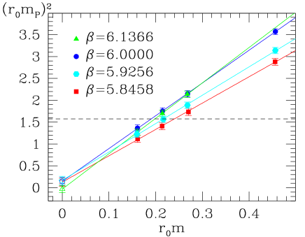
Figure 1: $(r_{0}m_{\rm P})^{2}$ as a function of $r_{0}m$. The horizontal dashed line represents the reference point $(r_{0}m_{\rm P})^{2}=1.5736$.

In order to compute $\widehat{Z}_{\rm S}$ according to eq. (2.2) we have to determine the quark mass at the reference point in units of $r_{0}$. In Fig. 1 we have plotted $(r_{0}m_{\rm P})^{2}$ as a function of $(r_{0}m)$ at all four $\beta$-values. As can be seen, the data are easily fitted by straight lines, but a non-zero intercept is found at all but the largest value of $\beta$: the pseudoscalar mass at zero bare quark mass differs from zero by $1-2$ standard deviations. Since the correlation function of the left-handed axial current is free from contributions of zero modes, they cannot be responsible for the non-zero intercept. We note however that the chiral fits yield $\chi^{2}/\rm dof$ below 1 even if the extrapolation is forced through the origin.

By performing local interpolations to the reference point using the three nearest data points and subsequently applying eq. (2.2), we obtain the values of $\widehat{Z}_{\rm S}$, which are tabulated at each $\beta$-value in Table 3. The typical accuracy of our determination is around 5%. It should be noted that the precision is partly limited by the accuracy of the published value of $U_{\rm{M}}$, which is about 3% [?]. We estimate that pushing the precision of our determination of $\widehat{Z}_{\rm S}$ to that level would require a four-fold increase in statistics.

$\beta$	$\widehat{Z}_{\rm S}$	$\widehat{Z}_{\rm P}$	$Z_{\rm A}$
$5.8458$	$1.28(6)$	$1.33(4)$	$1.710(5)$
$5.9256$	$1.19(7)$	$1.20(4)$	$1.611(3)$
$6.0000$	$1.05(5)$	$0.88(6)$	$1.553(2)$
$6.1366$	$1.01(4)$	$1.02(5)$	$1.478(2)$

Table 3: Non-perturbative determinations of $\widehat{Z}_{\rm S}$, $\widehat{Z}_{\rm P}$ and $Z_{\rm A}$.

In Fig. 3 we plot our results for $\widehat{Z}_{\rm S}$ versus $\beta$. It has become customary to represent results for renormalization factors at different values of the bare coupling by interpolating curves. Using a simple polynomial ansatz in $(\beta-6)$ yields

$$\widehat{Z}_{\rm S}(\beta)=1.045-0.899(\beta-6)+4.36(\beta-6)^{2},\qquad s=0.4.$$ (4.15)

This formula describes $\widehat{Z}_{\rm S}$ with an estimated error of 5% in the studied range of $\beta$, i.e. $5.8458\leq\beta\leq 6.1366$. We emphasize that our determination is valid only for the case $s=0.4$ in the definition of the Neuberger-Dirac operator, eqs. (3.6) and (3.7).

The perturbative expression for $\widehat{Z}_{\rm S}$ at one loop is

$$\widehat{Z}_{\rm S}^{\rm pt}(g_{0})=\frac{\kern 1.0pt\overline{\kern-1.0ptm\kern-1.0pt}\kern 1.0pt_{\rm\overline{MS\kern-0.35002pt}\kern 0.35002pt}(\mu)}{M}\left\{1+g_{0}^{2}\left[\frac{1}{2\pi^{2}}\ln(a\mu)+z_{\rm S}^{(1)}\right]+{\rm O}(g_{0}^{4})\right\},$$ (4.16)

where $z_{\rm S}^{(1)}=0.147107$ for our choice of $s=0.4$ [?,?]. The factor $\kern 1.0pt\overline{\kern-1.0ptm\kern-1.0pt}\kern 1.0pt_{\rm\overline{MS\kern-0.35002pt}\kern 0.35002pt}(\mu)/M$ was computed previously in [?]. The mean-field improved version of $\widehat{Z}_{\rm S}^{\rm pt}$ reads [?]

$$\widehat{Z}_{\rm S}^{\rm mf}(g_{0})=\frac{\kern 1.0pt\overline{\kern-1.0ptm\kern-1.0pt}\kern 1.0pt_{\rm\overline{MS\kern-0.35002pt}\kern 0.35002pt}(\mu)}{M}\left(\frac{1+s}{1+\tilde{s}}\right)\left\{1+g^{2}\left[\frac{1}{2\pi^{2}}\ln(a\mu)+z_{\rm S}^{(1)}+u_{0}^{(1)}\left(\frac{3-s}{1+s}\right)\right]\right\}\ ,$$ (4.17)

where $g^{2}=g_{0}^{2}/u_{0}^{4}$ is the boosted coupling, $\tilde{s}=3+(s-3)/u_{0}$, with $u_{0}^{4}$ being the average plaquette. The comparison of our numerical results for $\widehat{Z}_{\rm S}$ with perturbation theory is shown in Fig. 3. The mean-field improved perturbative expansion comes quite close to the non-perturbatively determined values for $\beta\;\raisebox{-2.58334pt}{$\stackrel{{\scriptstyle\textstyle{>}}}{{\sim}}$}\;6.0$ but falls short by more than 20% below $\beta=6.0$. Unsurprisingly, perturbation theory in the bare coupling $g_{0}^{2}$ fares a lot worse in the entire range of couplings studied here.

Figure 2: $\widehat{Z}_{\rm S}$ as a function of $\beta$. The solid line denotes the fit of eq. (4.15). The dotted and dashed curves represent the results of bare and mean-field improved perturbation theory at one loop order.

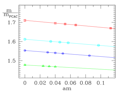
Figure 3: The quark mass dependence of $\frac{m}{m_{\rm PCAC}}$. The value of $\beta$ increases from top to bottom. $Z_{\rm A}$ is defined as the value of this ratio in the limit of vanishing quark mass.

The results for $\widehat{Z}_{\rm P}$, computed according to eq. (2.4), are listed alongside those for $\widehat{Z}_{\rm S}$ in Table 3. The renormalization conditions for $\widehat{Z}_{\rm S}$ and $\widehat{Z}_{\rm P}$ imply that the two must be identical up to effects of order $a^{2}$. Indeed, we observe hardly any difference at our level of accuracy, except at $\beta=6.0$. In our view, the most likely explanation for this deviation is a statistical fluctuation.

In order to include the pseudoscalar decay constant in the scaling tests described below we also computed the renormalization factor of the axial current, $Z_{\rm A}$. Using the PCAC relation and $Z_{\rm m}=1/Z_{\rm P}$ one can define

$$Z_{\rm A}=\lim_{m\to 0}\frac{m}{m_{\rm PCAC}}.$$ (4.18)

We found the ratio ${m}/{m_{\rm PCAC}}$ to depend only weakly on the bare mass (c.f. Fig. 3). $Z_{\rm A}$ could then be determined by extrapolating $m/m_{\rm PCAC}$ linearly in $m$ to the chiral limit.

5 The renormalized condensate

Having determined the renormalization factor of the scalar density in a range of bare couplings, we can now compute the renormalized condensate in the continuum limit, by combining the results for $\widehat{Z}_{\rm S}$ with estimates of the bare condensate.

In effective low-energy descriptions of QCD with $N_{\rm f}=3$ quark flavours, the quark condensate is identified with the low-energy constant $\Sigma$ via

$$-\left\langle\overline{\psi}\psi\right\rangle=\Sigma.$$ (5.19)

In the quenched theory, however, the condensate $-\langle\overline{\psi}\psi\rangle$ is not defined, owing to the presence of infrared divergencies as the chiral limit is approached [?]. Nevertheless, the low-energy constant $\Sigma$ can be determined in quenched QCD, for instance, by comparing lattice data of suitable quantities to expressions of Chiral Perturbation Theory or chiral Random Matrix Theory. Although in this case the identification of $\Sigma$ with the quark condensate is rather dubious, we shall nevertheless proceed to compute a renormalized “condensate”, by assuming that estimates of $\Sigma$ in the quenched theory renormalize like the scalar density.

Our input quantities are thus the renormalization factors $\widehat{Z}_{\rm S}$ of Table 3 and results for $\Sigma$, determined by matching the low-lying eigenvalues of the Dirac operator in the $\epsilon$-regime to the predictions of the chiral unitary random matrix model according to [?]

$$\left\langle\lambda_{k}\right\rangle_{\nu}{\Sigma}V=\left\langle\zeta_{k}\right\rangle_{\nu},\qquad k=1,2,\ldots$$ (5.20)

Here, $\langle\lambda_{k}\rangle_{\nu}$ is the expectation value of the $k$th eigenvalue in the topological sector with index $\nu$, and $\zeta_{k}$ denotes the $k$th scaled eigenvalue in the matrix model. In ref. [?] it was found that good agreement with random matrix behaviour is observed for lattice volumes $V$ of at least $(1.5\,{\rm fm})^{4}$. In other words, the value of $\Sigma$ extracted from eq. (5.20) depends neither on the particular eigenvalue, nor on the topological sector, within statistical errors.

Using the results for $\Sigma$ from Table 3 of [?] (i.e. the runs labelled $\rm B_{0},B_{1}$ and $\rm B_{2}$), supplemented by our data at $\beta=5.9256$, we plot the renormalization group invariant condensate $\widehat{\Sigma}$ in units of $r_{0}$ versus $(a/r_{0})^{2}$ in Fig. 5. If the non-perturbative estimates for $\widehat{Z}_{\rm S}$ are used, the results for $r_{0}^{3}\widehat{\Sigma}$ show a remarkably flat behaviour, which not only indicates small residual cutoff effects, but is also consistent with the expectation that the leading lattice artefacts of our fermionic discretization should be of order $a^{2}$.

Figure 5 also reveals that employing mean-field improved perturbation theory for $\widehat{Z}_{\rm S}$ produces a significant slope in $r_{0}^{3}\widehat{\Sigma}$ as the continuum limit is approached. Although this procedure apparently yields a consistent value of $r_{0}^{3}\widehat{\Sigma}$ in the continuum limit, it is equally obvious that the perturbatively renormalized result serves as a poor estimate for the condensate at non-zero lattice spacing.

Figure 4: Continuum extrapolation of $r_{0}^{3}\widehat{\Sigma}$. Full circles denote the results obtained using non-perturbative renormalization factors, while open squares represent values resulting from applying mean-field improved perturbation theory.

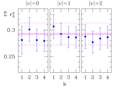
Figure 5: The variation of $r_{0}^{3}\widehat{\Sigma}$ in the continuum limit, arising from choosing different eigenvalues and topological sectors in the determination of the bare condensate. The solid and dashed lines represent the result for $k=2,\,|\nu|=1$ which is used for our main result.

Our results for $r_{0}^{3}\widehat{\Sigma}$ at all values of $\beta$ and in the continuum limit are listed in Table 4. Here we have used $\Sigma$ as determined from $\langle\lambda_{k}\rangle_{\nu}$ for $k=2$ and $|\nu|=1$. We note that the variation in the value of $r_{0}^{3}\widehat{\Sigma}$ from choosing different $\lambda_{k}$’s and topological sectors is well within the statistical fluctuations after taking the continuum limit. This is illustrated in Fig. 5, where we plot the continuum results for all possible choices of $\lambda_{k}$ and $|\nu|$. We emphasize that this variation should not be regarded as a systematic uncertainty, since all choices are equivalent, if random matrix theory does indeed give an accurate description of the low-lying eigenvalues, and hence we refrain from quoting an additional error.

$\beta$	$r_{0}^{3}\widehat{\Sigma}$	$r_{0}F_{\rm K}$	$r_{0}m_{\rm K^{*}}$
$5.8458$	$0.282(14)$	$0.296(6)$	$2.209(89)$
$5.9256$	$0.285(16)$	$0.301(7)$	$2.403(95)$
$6.0000$	$0.275(14)$	$0.293(5)$	$2.413(66)$
$6.1366$	$0.294(13)$	$0.297(7)$	$2.328(165)$
$\infty$	${\it 0.293(21)}$	${\it 0.294(9)}$	${\it 2.32(29)}$

Table 4: Renormalization group invariant quark condensate, kaon decay constant and $K^{*}$-mass, in units of $r_{0}$.

Our result in the continuum limit is thus

$$r_{0}^{3}\widehat{\Sigma}=0.293\pm 0.021$$ (5.21)

for the renormalization group invariant condensate. In the ${\rm\overline{MS\kern-0.50003pt}\kern 0.50003pt}$-scheme at $2\,{\rm GeV}$ we obtain after division by $\kern 1.0pt\overline{\kern-1.0ptm\kern-1.0pt}\kern 1.0pt_{\rm\overline{MS\kern-0.35002pt}\kern 0.35002pt}(2\,{\rm GeV})/M=0.72076$ [?] the value

$$r_{0}^{3}\Sigma_{\rm\overline{MS\kern-0.35002pt}\kern 0.35002pt}(2\,{\rm GeV})=0.406\pm 0.029.$$ (5.22)

These are the main results of our calculation. To our knowledge, these are the first estimates of a quantity in the continuum limit, computed using overlap fermions. We emphasize that the quoted errors include all uncertainties, except those due to quenching.

As is well known, the calibration of the lattice spacing is ambiguous in the quenched approximation, and thus any conversion into physical units is only illustrative. Here we perform such a conversion using either the kaon decay constant or the nucleon mass to set the scale. Ref. [?] quotes

$$r_{0}F_{\rm K}\sqrt{2}=0.415\pm 0.009,\qquad F_{\rm K}=113\,{\rm MeV},$$ (5.23)

in the continuum limit, while a continuum extrapolation of the nucleon mass data of [?] in units of $r_{0}$ yields

$$r_{0}m_{\rm N}=2.670\pm 0.042,\qquad m_{\rm N}=939.6\,{\rm MeV}.$$ (5.24)

For the condensate in the ${\rm\overline{MS\kern-0.50003pt}\kern 0.50003pt}$-scheme at $2\,{\rm GeV}$ we then obtain

$$\Sigma_{\rm\overline{MS\kern-0.35002pt}\kern 0.35002pt}(2\,{\rm GeV})=\left\{\begin{array}[]{ll}(285\pm 9\,{\rm MeV})^{3},&\quad\hbox{scale set by $F_{\rm K}$}\\ (261\pm 8\,{\rm MeV})^{3},&\quad\hbox{scale set by $m_{\rm N}$}\end{array}\right..$$ (5.25)

These findings are consistent with previous observations that the typical scale ambiguity for a quantity with mass dimension equal to one is of the order of 10%. Recent calculations of the renormalized condensate [?,?,?,?,?,?,?,?,?,?] yield similar values compared to our results.

6 Further scaling tests

The leading cutoff effects of fermionic discretizations based on the Ginsparg-Wilson relation are expected be of order $a^{2}$, and indeed, this expectation has been confirmed in our scaling study of the quark condensate. In this section we shall extend our analysis of cutoff effects to quantities like the pseudoscalar decay constant and the meson mass in the vector channel.

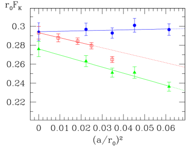
Figure 6: Continuum extrapolation of $r_{0}F_{\rm K}$. Full circles denote our results, while the open squares are the data of [?], employing O($a$) improved Wilson fermions. The full triangles are our data with $Z_{\rm A}$ from mean-field improved perturbation theory.

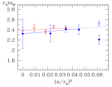
Figure 7: Scaling behaviour of $r_{0}m_{\rm K^{*}}$. The meaning of the full circles and open squares is as in Fig. 7. The open circle results from an alternative fit with a fit range of $x_{0}/a\in[5,11]$ instead of $x_{0}/a\in[8,11]$ (full circle).

To this end we have assumed that $aF_{\rm P}^{\rm bare}$ and $am_{\rm V}$ depend linearly on $(am_{\rm P})^{2}$ and performed a linear interpolation to the point where $(r_{0}m_{\rm P})^{2}=(r_{0}m_{\rm K})^{2}=1.5736$. Thus, our aim is to investigate the scaling behaviour of $F_{\rm K}$ and $m_{\rm K^{*}}$. The renormalized kaon decay constant is obtained after multiplication with the factor $Z_{\rm A}$ listed in Table 3. In Table 4 we have compiled the results for $r_{0}F_{\rm K}$ and $r_{0}m_{\rm K^{*}}$ at the various values of $\beta$, as well as in the continuum limit. The corresponding continuum extrapolations are plotted in Figures 7 and 7.

For the kaon decay constant we observe a flat approach to the continuum limit, consistent with a linear fit in $(a/r_{0})^{2}$, provided that the non-perturbative estimate for $Z_{\rm A}$ is used. The perturbatively renormalized $F_{\rm K}$ is subject to larger lattice artefacts, and the resulting continuum value is roughly consistent. In Fig. 7 we also show the continuum extrapolation of the same quantity from ref. [?], where $r_{0}F_{\rm K}$ was computed using O($a$) improved Wilson fermions. In the continuum limit our data agree remarkably well with those of ref. [?], but for overlap fermions the residual cutoff effects at lattice spacings of around $0.1\,{\rm fm}$, i.e. at $(a/r_{0})^{2}\approx 0.035$, are apparently much smaller.

The scaling behaviour of the $K^{*}$ mass is also flat, except at our coarsest lattice spacing. A closer inspection of our fits to the two-point function shows that the value of $am_{\rm V}$ at $\beta=5.8458$ depends strongly on the chosen fit range. Extending the fit interval to smaller timeslices leads to a significant increase in the value of $r_{0}m_{\rm K^{*}}$, as indicated in Fig. 7. Owing to the uncertainty in the value of $r_{0}m_{\rm K^{*}}$ as a result of using different fit intervals, we exclude the coarsest lattice from the continuum extrapolation, despite the fact that the alternative result is apparently consistent with a linear behaviour up to $(a/r_{0})\approx 0.06$. Nevertheless we also confirm good scaling behaviour for the vector mass; as our values for $\beta>5.8458$ are mutually consistent with each other, as well as with the results of ref. [?].

7 Conclusions

We have presented the first comprehensive scaling study of quantities computed using overlap fermions. A major part of our calculation was devoted to the determination of the renormalization factor $\widehat{Z}_{\rm S}$ of the scalar density. Thereby we were able to present a conceptually clean determination of the renormalized low-energy constant $\Sigma$ in the continuum limit of quenched QCD, with a total accuracy of 7%.

Besides studying the continuum extrapolation of $r_{0}^{3}\widehat{\Sigma}$ we also performed scaling studies of the pseudoscalar decay constant and the mass in the vector channel. For all three quantities computed using overlap quarks we observed an excellent scaling behaviour, resulting in a flat approach to the continuum limit. This is signified by the fact that the results in Table 4 at any finite value of $\beta$ and in the continuum limit are practically the same, at least at our level of accuracy. We note, however, that a flat continuum behaviour is only observed for $\widehat{\Sigma}$ and $F_{\rm K}$, if non-perturbative estimates of the respective renormalization factors are employed. Our values for $r_{0}F_{\rm K}$ and $r_{0}m_{\rm K^{*}}$ in the continuum limit are in very good agreement with those of refs. [?,?].

Owing to their good scaling properties, overlap fermions are an attractive discretization for the computation of phenomenologically interesting quantities, despite the large numerical effort involved in their simulation.

References

- [1] L. H. Karsten and J. Smit, Nucl. Phys. B183 (1981) 103; M. Bochicchio, L. Maiani, G. Martinelli, G.C. Rossi and M. Testa, Nucl. Phys. B262 (1985) 331;
- [2] H. Neuberger, Phys. Lett. B417 (1998) 141; ibid. B427 (1998) 353
- [3] P. Hernández, K. Jansen, L. Lellouch and H. Wittig, JHEP 0107 (2001) 018
- [4] L. Giusti, F. Rapuano, M. Talevi and A. Vladikas, Nucl. Phys. B538 (1999) 249
- [5] P. Hernández, K. Jansen and L. Lellouch, Phys. Lett. B469 (1999) 198
- [6] T. Blum et al., Phys. Rev. D69 (2004) 074502
- [7] MILC Collaboration (T. DeGrand), Phys. Rev. D63 (2001) 034503; Phys. Rev. D64 (2001 117501
- [8] L. Giusti, C. Hoelbling and C. Rebbi, Phys. Rev. D64 (2001) 114508 [Erratum-ibid. D65 (2002) 079903]
- [9] P. Hernández, K. Jansen, L. Lellouch and H. Wittig, Nucl. Phys. B (Proc. Suppl.) 106 (2002) 766
- [10] P. Hasenfratz, S. Hauswirth, T. Jörg, F. Niedermayer and K. Holland, Nucl. Phys. B643 (2002) 280
- [11] D. Bećirević and V. Lubicz, Phys. Lett. B600 (2004) 83
- [12] V. Gimenez, V. Lubicz, F. Mescia, V. Porretti and J. Reyes, Eur. Phys. J. C 41, 535 (2005)
- [13] C. McNeile, Phys. Lett. B 619, 124 (2005)
-
[14]
C.W. Bernard and M.F.L. Golterman,
Phys. Rev. D 46 (1992) 853
,
S.R. Sharpe, Phys. Rev. D 46 (1992) 3146 ,
P.H. Damgaard and K. Splittorff, Phys. Rev. D 62 (2000) 054509 ,
P.H. Damgaard, Nucl. Phys. B 608 (2001) 162 - [15] P.H. Ginsparg and K.G. Wilson, Phys. Rev. D25 (1982) 2649
- [16] M. Lüscher, Phys. Lett. B428 (1998) 342
- [17] R. Sommer, Nucl. Phys. B411 (1994) 839; ALPHA Collaboration (M. Guagnelli et al.), Nucl. Phys. B535 (1998) 389; S. Necco and R. Sommer, Nucl. Phys. B622 (2002) 328
- [18] ALPHA/UKQCD Collaborations (J. Garden et al.), Nucl. Phys. B571 (2000) 237
- [19] ALPHA Collaboration (S. Capitani et al.), Nucl. Phys. B544 (1999) 669
- [20] L. Giusti, Ch. Hoelbling, M. Lüscher and H. Wittig, Comput. Phys. Commun. 153 (2003) 31
- [21] Y. Saad, Iterative methods for sparse linear systems, 2nd ed. (SIAM, Philadelphia, 2003); see also http://www-users.cs.umn.edu/~saad
- [22] Jan Wennekers, Ph.D. thesis, in preparation
- [23] L. Giusti, M. Lüscher, P. Weisz and H. Wittig, JHEP 0311 (2003) 023
- [24] W. Bietenholz, T. Chiarappa, K. Jansen, K. I. Nagai and S. Shcheredin, JHEP 0402 (2004) 023
- [25] L. Giusti, P. Hernández, M. Laine, P. Weisz and H. Wittig, JHEP 0404 (2004) 013
- [26] T. DeGrand and S. Schaefer, Comput. Phys. Commun. 159 (2004) 185
- [27] UKQCD Collaboration (C.R. Allton et al.), Phys. Rev. D47 (1993) 5128
- [28] C. Alexandrou, E. Follana, H. Panagopoulos and E. Vicari, Nucl. Phys. B580 (2000) 394
- [29] S. Capitani and L. Giusti, Phys. Rev. D62 (2000) 114506
- [30] CP-PACS Collaboration (S. Aoki et al.), Phys. Rev. D67 (2003) 034503
-
[31]
K. Jansen, M. Papinutto, A. Shindler, C. Urbach and I. Wetzorke,
arXiv:hep-lat/0507010.