The $\Upsilon$ spectrum and $m_{b}$ from full lattice QCD

Abstract

We show results for the $\Upsilon$ spectrum calculated in lattice QCD including for the first time vacuum polarization effects for light $u$ and $d$ quarks as well as $s$ quarks. We use gluon field configurations generated by the MILC collaboration. The calculations compare the results for a variety of $u$ and $d$ quark masses, as well as making a comparison to quenched results (in which quark vacuum polarisation is ignored) and results with only $u$ and $d$ quarks. The $b$ quarks in the $\Upsilon$ are treated in lattice Nonrelativistic QCD through NLO in an expansion in the velocity of the $b$ quark. We concentrate on accurate results for orbital and radial splittings where we see clear agreement with experiment once $u$, $d$ and $s$ quark vacuum polarisation effects are included. This now allows a consistent determination of the parameters of QCD. We demonstrate this consistency through the agreement of the $\Upsilon$ and $B$ spectrum using the same lattice bare $b$ quark mass. A one-loop matching to continuum QCD gives a value for the $b$ quark mass in full lattice QCD for the first time. We obtain $m_{b}^{\overline{MS}}(m_{b}^{\overline{MS}})$ = 4.4(3) GeV. We are able to give physical results for the heavy quark potential parameters, $r_{0}$ = 0.469(7) fm and $r_{1}$ = 0.321(5) fm. Results for the fine structure in the spectrum and the $\Upsilon$ leptonic width are also presented. We predict the $\Upsilon-\eta_{b}$ splitting to be 61(14) MeV, the $\Upsilon^{\prime}-\eta_{b}^{\prime}$ splitting as 30(19) MeV and the splitting between the $h_{b}$ and the spin-average of the $\chi_{b}$ states to be less than 6 MeV. Improvements to these calculations that will be made in the near future are discussed.

I Introduction

The calculation of the spectrum of bottomonium and charmonium states is a key one for lattice QCD, for several reasons:

• There are many ‘gold-plated’ (narrow, stable and experimentally well-characterised) states whose masses can be calculated accurately in lattice QCD.

• Splittings in the spectrum have particularly good properties to use for determining the scale of the theory, $\Lambda_{QCD}$. In lattice QCD determining this scale is equivalent to knowledge of the lattice spacing and it is an important first calculation that must be done before quoting other dimensionful quantities on the lattice such as hadron masses, or giving a scale to $\alpha_{s}$.

• The bottomonium and charmonium calculations provide a test of the lattice QCD actions used for the heavy $b$ and $c$ quarks. These can then be used for the $B$ and $D$ physics results needed for the experimental programme charged with testing the consistency of CP violation in the Standard Model. Lattice QCD numbers are critical, for example, to push down the limits on determination of the elements of the CKM matrix to the few percent level.

• The control of systematic errors from the lattice for heavyonium masses is well developed and the results are statistically very precise. Vacuum polarisation effects for heavy quarks are not included because they are known perturbatively to have very little effect. This makes the tuning of the heavy quark mass much simpler than that of light quark masses. The heavyonium spectrum is sensitive to $u$, $d$, and $s$ quark vacuum polarisation effects, but is not very sensitive to the actual values of the light quark masses, once they are low enough. All of these points make calculations of heavyonium masses in the presence of light quark vacuum polarization relatively simple, and a good test of lattice methods.

We need to achieve statistical and systematic errors of a few percent in order for lattice QCD to provide useful information for the particle physics programme not obtainable by other methods. New results us ; ourms ; milc3 ; bc ; dsemi indicate that this is starting to be possible, building on many years of work by the lattice community to understand the sources of error in lattice calculations. The developments that have enabled this progress are: improved actions, the inclusion of light sea quarks (i.e. light quark vacuum polarization effects) and effective theories for handling heavy quarks. In particular the inclusion of $u$, $d$, and $s$ sea quarks with light $u$ and $d$ quark masses has produced agreement with experiment for a range of hadron masses for the first time us . A key component of this, for the reasons above, has been a set of results on the $\Upsilon$ spectrum and we describe these in more detail here.

Section II describes details of the lattice calculations and section III gives the results obtained. In sections IV and V we describe the analysis that allows the extraction of the lattice spacing and we compare the spectrum obtained to experiment. In section VI we describe the determination of the $b$ quark mass from the results. In sections VII and VIII we discuss the fine structure in the spectrum and the determination of the leptonic width of the $\Upsilon$ and its radial excitations. We conclude in section IX with a discussion of further improvements that will be made, particularly to these last two calculations.

II The lattice calculation

The bottomonium spectrum is obtained by calculating correlators for bottomonium hadrons on configurations of gluon fields generated by a Monte Carlo procedure. The gluon field configurations in an ensemble are generated with a probability distribution given by $\exp(-S_{QCD})$ where $S_{QCD}$ is the QCD action. Averaging over results on an ensemble then gives the Feynman Path Integral result for the bottomonium correlator. First we describe the different ensembles of gluon field configurations that we have used and then the method for calculating the bottomonium correlators. We will then estimate the size of systematic errors in the calculation and finally discuss the fitting procedure which enables us to obtain energies and amplitudes for different states from the correlators.

The ensembles of gluon field configurations were generated by the MILC collaboration milc1 ; milc2 . Different ensembles include the effect of zero, two and three flavors of sea quarks. Ensembles with zero flavors of sea quarks are called ‘quenched’, and those with sea quarks included are called ‘unquenched’ (or ‘dynamical’). The ensembles with three flavors are most interesting from a physical point of view because sea $u$, $d$, and $s$ quarks are an important component of the vacuum of QCD in the real world. The MILC collaboration has made ensembles with a range of masses for the sea $u$ and $d$ quark masses (which are taken to be equal) down to much lighter values than before and within reach of their real world values. The ensembles in which the sea $u$ and $d$ quarks are much lighter than the sea $s$ quark will be called ‘2+1 flavor’ ensembles. The inclusion of light sea quarks has been made possible by a formulation for light quarks on the lattice called improved staggered (asqtad) quarks impstagg . Apart from being numerically very fast, this formulation of the QCD action for light quarks is also very accurate. It has all sources of discretisation error removed to $\cal{O}$$(\alpha_{s}a^{2})$, where $a$ is the lattice spacing and $\alpha_{s}$ is the QCD coupling constant. The gluonic piece of the action is also simulated with a very accurate discretisation of QCD which has errors at $\cal{O}$$(\alpha_{s}^{2}a^{2})$ apart from effects from sea quarks, expected to be small, which feed in at $\cal{O}$$(\alpha_{s}a^{2})$ glue . In order to check the effect of discretisation errors, two sets of ensembles are available with lattice spacing values around 0.12fm and 0.09fm milc2 , and recently a further, coarser set, has become available with a lattice spacing around 0.17fm.

The physical volumes of the configurations are large, $(2.5{\rm fm})^{3}$, so we do not expect significant errors from having a finite volume. Some analysis of finite volume errors has been done for light hadrons by the MILC collaboration milc2 and no significant effect was found on these volumes. $\Upsilon$ states are smaller than light hadrons in general so we expect even less of an effect here.

Lattice $n_{f}$ $\beta$ $am_{l},am_{s}$ $u_{0L}$ $aM^{0}_{b}$ $n_{conf}$ $n_{orig}$ $16^{3}\times 48$ super-coarse 2+1 6.458 0.0082,0.082 0.814 4.0 461 8 $20^{3}\times 64$ coarse 0 8.0 - 0.856 2.8 210 16 2 7.2 0.02,- 0.845 2.8 210 16 3 6.85 0.05,0.05 0.8391 2.8 210 8 2+1 6.81 0.03,0.05 0.8378 2.8 210 16 2+1 6.79 0.02,0.05 0.837 2.8 210 16 2+1 6.76 0.01,0.05 0.836 2.8 210 16 $28^{3}\times 96$ fine 0 8.4 - 0.8652 1.95 210 16 2+1 7.11 0.0124, 0.031 0.855 1.95 210 16 2+1 7.09 0.0062, 0.031 0.8461 1.95 159 16,12*

Table 1: Parameters and details of MILC configurations used for $\Upsilon$ correlator calculations. $n_{f}$ is the number of sea flavors, varying from 0 (quenched) through 2 (degenerate $u$ and $d$ only) and 3 (degenerate $u$, $d$ and $s$) to the most physical 2+1 (degenerate $u$ and $d$ and more massive $s$). $\beta$ is the bare gauge coupling parameter in the gluon action, $10/g^{2}$. $am_{l}$, $am_{s}$ are the light sea $u/d$ and $s$ quark masses respectively in lattice units (using the MILC convention for quark mass, see ourms ). $u_{0L}$ is our estimate of the maximal trace link in lattice Landau gauge used to tadpole-improve fields in our NRQCD action. $a\mbox{$M_{b}^{0}$}$ is the bare $b$ quark mass in lattice units. $n_{conf}$ is the number of configurations from the MILC ensemble used in our calculation with $n_{orig}$ origins for the heavy quark propagators per configuration. *For 92 of the 159 configurations, only 12 origins were used instead of 16. Tables 8, 9 and 10 give our lattice spacing determinations for these ensembles; they are approximately 0.17fm for the super-coarse ensemble, 0.12fm for the coarse ensembles and 0.09fm for the fine ensembles. The pion masses corresponding to the $u/d$ quark mass on the most chiral (i.e. lightest $u/d$ mass) fully unquenched ensemble in each set are 270 MeV on the super-coarse milcprivate , 360 MeV on the coarse and 330 MeV on the fine ensembles milc2 .

The sets of ensembles of gluon field configurations on which we have calculated bottomonium correlators are given in Table 1. The ensembles within the ‘coarse’ set and the ‘fine’ set are matched to have approximately the same lattice spacing to separate discretisation effects from effects of changing the sea quark mass. There are results for a variety of $u/d$ quark masses, heavier than the real world values and we will examine the dependence of our results on the $u/d$ quark mass, aiming for conclusions that are relevant to the physical (chiral) limit where the $u/d$ quark mass is very small. The sea $s$ quark mass takes only one value here, which is only approximately tuned (for example, it is slightly high on the coarse set of ensembles). Again, whether this has any impact or not depends on how sensitive results are to the sea quark mass. The $b$ quarks are treated only as valence quarks because their effect in the sea should be negligible, being suppressed by inverse powers of the $b$ quark mass nobes . We also neglect $c$ quark vacuum polarization effects for the same reason.

For the valence $b$ quarks in the $\Upsilon$ system we use lattice Nonrelativistic QCD (NRQCD) which has been developed over many years thacker ; nakhleh ; upspaper to handle well the physics of heavy quark systems on the lattice. The main point here is that the $b$ quark has a mass which is larger than 1 in lattice units and therefore momentum scales of order the mass cannot be simulated without large discretisation errors. On the other hand such large scales do not need to be simulated on the lattice because they are irrelevant to the internal dynamics of the bound state which sets the mass splittings. The $b$ quark is non-relativistic inside its bound states ($v_{b}^{2}\approx 0.1$ for the $\Upsilon$) and so a non-relativistic expansion of the QCD action is appropriate that accurately handles scales of the order of typical momenta and kinetic energies inside these states. Non-relativistic QCD can be matched to full QCD order by order in the expansion in $v^{2}$ and $\alpha_{s}$.

The lattice NRQCD Hamiltonian that we use is given by

$$H = H_{0}+\delta H;$$

$$H_{0} = -{\Delta^{(2)}\over 2\mbox{$M_{b}^{0}$}},$$

$$\delta H = -c_{1}\frac{(\Delta^{(2)})^{2}}{8(\mbox{$M_{b}^{0}$})^{3}}+c_{2}\frac{ig}{8(\mbox{$M_{b}^{0}$})^{2}}\left({\bf{\bf\Delta}}\cdot{\bf E}-{\bf E}\cdot{\bf{\bf\Delta}}\right)$$ (1)

$$-c_{3}\frac{g}{8(\mbox{$M_{b}^{0}$})^{2}}\mbox{\boldmath$\sigma$}\cdot({\bf{\bf\Delta}}\times\tilde{{\bf E}}-\tilde{{\bf E}}\times{\bf{\bf\Delta}})$$

$$-c_{4}\frac{g}{2\mbox{$M_{b}^{0}$}}\,\mbox{\boldmath$\sigma$}\cdot\tilde{{\bf B}}+c_{5}\frac{a^{2}{\Delta^{(4)}}}{24\mbox{$M_{b}^{0}$}}$$

$$-c_{6}\frac{a(\Delta^{(2)})^{2}}{16n(\mbox{$M_{b}^{0}$})^{2}}.$$

Here ${\bf\Delta}$ is the symmetric lattice derivative and ${\Delta^{(4)}}$ is the lattice discretisation of the continuum $\sum_{i}D_{i}^{4}$. $M_{b}^{0}$ is the bare $b$ quark mass. The spin-independent terms contribute to the (spin-averaged) differences in mass between radial and orbital excitations in the spectrum and the ground-state. Spin-independent terms are included through next-to-leading order above with the Darwin and $p^{4}$ relativistic corrections. We will now discuss remaining sources of systematic error in turn in the radial and orbital splittings and estimate their size.

Correction relativistic radiative radiative Total kinetic Darwin relativistic + radiative Form $\delta p^{6}/(M_{b})^{5}$ $\alpha_{s}\delta p^{4}/4(M_{b})^{3}$ $4\pi\alpha_{s}^{2}\psi(0)^{2}/(3M_{b}^{2})$ Est. %age in $2S-1S$ supercoarse 0.5 0.5 0.5 1.0 coarse 0.5 0.4 0.3 0.7 fine 0.5 0.3 0.2 0.6 Est. %age in $1P-1S$ supercoarse 1.0 2.0 1.0 2.5 coarse 1.0 1.5 0.7 2.0 fine 1.0 1.2 0.4 1.5

Table 2: An estimate of systematic errors in the $2S-1S$ and $1P-1S$ splittings in the $\Upsilon$ in our lattice QCD calculation arising from missing higher order relativistic and radiative corrections to the NRQCD action that we use.

Correction discretisation in discretisation in discretisation in Total NRQCD action (i) NRQCD action (ii) gluon action discretisation Form $\alpha_{s}a\delta p^{4}/8n(M_{b})^{2}$ $\alpha_{s}a^{2}\delta p_{i}^{4}/12M_{b}$ $4\pi\alpha_{s}a^{2}\psi(0)^{2}/15$ Est. %age in $2S-1S$ supercoarse 0.5 1.7 1.0 2.0 coarse 0.3 0.7 0.5 1.0 fine 0.2 0.3 0.2 0.4 Est. %age in $1P-1S$ supercoarse 2 7 3 8 coarse 1.2 3 1.7 4 fine 0.7 1.2 0.5 1.5

Table 3: An estimate of systematic errors in the $2S-1S$ and $1P-1S$ splittings in the $\Upsilon$ in our lattice QCD calculation arising from discretisation errors in the NRQCD and gluon actions.

II.1 Systematic errors

Relativistic errors. Errors from missing higher orders in the relativistic expansion should be $\cal{O}$$(v^{4})=1\%$ in the radiative and orbital splittings in principle. However, this does not allow for the fact that the error is set by the difference in the expectation value of the relativistic correction in the two states that make up the splitting. Estimates of the expectation value of powers of $p$ in a potential model show that the $2S$ and $1S$ states are similar enough, and have similar enough expectation values, that the error in the difference between these states is significantly less than the naive expectation. We take the systematic error from relativistic corrections to be 0.5% for the $2S-1S$ splitting and 1% for the the $1P-1S$ splitting here. These sources of error are tabulated in Table 2.

Radiative errors. We must also consider missing radiative corrections to the terms that we are including in the NRQCD action. These are represented by the coefficients $c_{i}$ that are required to match full QCD by taking account of gluon radiation above the lattice cut-off, missing from the lattice theory. The $c_{i}$ coefficients take the form $1+c_{i}^{(1)}\alpha_{s}+\ldots$, where $c_{i}^{(1)}$ is a function of the bare heavy quark mass in lattice units, $M_{b}^{0}a$. Calculation of the $c_{i}^{(1)}$ is in progress for this action. They were calculated earlier for a similar but different NRQCD (and gluon) action colin2 and found to have a value around 0.5 for $aM_{b}^{0}>1$. Here we have set the $c_{i}$ to 1, giving expected systematic errors of $\cal{O}$$(v^{2}\alpha_{s})=2-3\%$ in spin-independent splittings from a very naive analysis. A more sophisticated analysis, as for the relativistic corrections, uses the expectation value of $p^{4}$ in the different states from a potential model and calculates $2\alpha_{s}\delta(p^{4})/8M_{b}^{3}$, where $\delta(p^{4})$ is the difference in $p^{4}$ values appropriate to the splitting and the factor of 2 comes from having 2 $b$ quarks in an $\Upsilon$. The error estimates that this gives are shown in Table 2. The effect of the Darwin term, ${\bf{\bf\Delta}}\cdot{\bf E}$, can be estimated in a potential model by adding a delta function of appropriate strength ($\nabla^{2}V$) at the origin. The systematic error from missing radiative corrections to the Darwin term is then $4\pi\alpha_{s}^{2}\psi^{2}(0)/(3M_{b}^{2})$ where $\psi^{2}(0)$ is the square of the ‘wavefunction at the origin’. We estimate this using our results in section VIII and tabulate the estimates in Table 2. We can then add all our estimates together in quadrature to obtain a total estimated systematic error from relativistic and radiative corrections and this is also given in Table 2. The maximum error is 2.5% for the $1P-1S$ splitting on the super-coarse lattices.

Note that we have tadpole-improved all the gauge fields appearing above by dividing the gluon fields, $U_{\mu}$, by a parameter $u_{0}$ which cancels, in a mean-field way, the effect of a disparity between the lattice and continuum gluon fields induced by the fact that the lattice field is exponentially related to the continuum field tadimp . Extra tadpole diagrams appear in the quark-gluon coupling on the lattice and these take a fairly universal form, allowing a cancellation by $u_{0}$. $u_{0}$ should be a measure of the difference between $U_{\mu}$ and the unit matrix, but is not uniquely specified. Here (as given in Table 1) we use $u_{0L}$, an estimate of the trace of the average $U_{\mu}$ field in lattice Landau gauge (which maximises this trace). Subsequent determinations of the trace of the Landau link milcprivate have shown that the values used on the fine ensemble are underestimates by about 1%. In Figure 1, however, we show that using a rather different value of $u_{0}$ based on the plaquette ($u_{0P}=\sqrt[4]{plaq}$ = 0.8677 milc1 on the coarse 2+1 flavor 0.01/0.05 ensemble used for comparison) has no discernible effect (less than our 1.5% statistical error) on spin-independent, radial and orbital, splittings comment . This also lends support to the idea that the $c_{i}$ are not very different from 1 because they must perturbatively correct for the different $u_{0}$ factors. Without tadpole-improvement the $c_{i}$ would be very different from 1.

Discretisation errors. The Hamiltonian above, Equation 1, also includes terms which correct for discretisation errors in the leading order spatial derivative (squared) and temporal derivative. These are the terms multiplied by $c_{5}$ and $c_{6}$ respectively. Note that both terms have large numerical factors in the denominator. As above, $c_{5}$ and $c_{6}$ are set to 1 here, and the systematic error comes from neglected radiative corrections. The $\cal{O}$$(\alpha_{s})$ pieces of $c_{5}$ and $c_{6}$ were calculated in  colin2 . Indeed $c_{1}$ and $c_{6}$ are not independent since these terms can be combined. Both $c_{5}^{(1)}$ and $c_{6}^{(1)}$ were found to be 0.5, i.e. $\cal{O}$$(1)$, as expected. The expected systematic error in spin-independent splittings is then $\cal{O}$$(\alpha_{s}(a\mbox{$M_{b}^{0}$})^{2}v^{2}/12)=5\%\times(a^{2}\,{\rm in\,GeV^{-2}})$ and $\cal{O}$$(\alpha_{s}(a\mbox{$M_{b}^{0}$})v^{2}/8n)<1\%\times(a\,{\rm in\,GeV})$ from a naive analysis. The more sophisticated analysis as above uses estimates of $p^{4}$ in a potential model and the results are tabulated in Table 3. Corrections which are higher order in $a$ will have an even smaller effect because the additional powers of $a\mbox{$M_{b}^{0}$}$ will come with additional powers of $v^{2}$. The Darwin term also contributes to the discretisation errors and an estimate of this is in progress. Preliminary results nobespriv suggest that it has a negligible coefficient and so we do not include an error for it here. There are, however, additional discretisation errors coming from the gluon action. These were previously estimated for unimproved glue in earlier work oldalpha . Because the error is proportional to the difference in the square of the wave function at the origin, again we find a bigger systematic error in the $1P-1S$ splitting than in the $2S-1S$. This correction is now reduced by a factor of $\alpha_{s}$ for the improved glue configurations we are working with here. We give estimates for its size in Table 3. The total systematic error estimated from discretisation effects is also given in this Table. The error is sizeable on the super-coarse lattices and dominates that from missing relativistic and radiative corrections. On the fine lattices the estimated discretisation error is only 0.4% in the $2S-1S$ splitting, about the same size as the relativistic/radiative errors.

From our error analysis it is clear that we should use the $2S-1S$ splitting to set the lattice spacing, despite the fact that it is somewhat harder to obtain precise results. Then the systematic error above is smaller than our statistical error on all except the super-coarse ensemble. Because we have results at three different values of the lattice spacing we can assess how good our estimates of systematic errors are, and we will do that below.

It is interesting to note that the effect of sea $c$ and $b$ quarks is to modify the coefficients of the higher order improvement terms in the gluon action nobes at $\cal{O}$$(\alpha_{s})$. The additional coefficients are very small, 0.025$\alpha_{s}$ for the rectangle term for $am_{c}\approx 1$, so from the arguments above we can see that their effect would be entirely negligible in spin-independent splittings.

$E$ and $B$ are the chromoelectric and chromomagnetic fields. They are generally defined by standard cloverleaf operators (tadpole-improved) but here we use improved operators $\tilde{E}$ and $\tilde{B}$ for the $E$ and $B$ operators which appear in the spin-dependent terms. These terms are only included at leading order in the Hamiltonian above and therefore we expect systematic errors in the spin-splittings of $\cal{O}$$(v^{2})=10\%$ from higher orders in the relativistic expansion and $\cal{O}$$(\alpha_{s})=20\%$ from perturbative corrections in $c_{3}$ and $c_{4}$. Previous studies scaling showed that $a^{2}$ errors in the cloverleaf operators could have a substantial effect for the fine structure splittings, such as the hyperfine splitting, presumably because this splitting is sensitive to short distances and therefore rather large momenta, $pa$, for the quark. Here we therefore attempt to ameliorate this effect by correcting the cloverleaf operator in these terms for the leading discretisation errors. This is done by the following replacement nakhleh ( using the corrected tadpole-improvement factors from clover ):

$$F_{\mu\nu}(x) \rightarrow \frac{5}{3}F_{\mu\nu}(x)-\frac{1}{6}[U_{\mu}(x)F_{\mu\nu}(x+a\hat{\mu})U^{{\dagger}}_{\mu}(x)$$ (2)

$$+ U^{{\dagger}}_{\mu}(x-a\hat{\mu})F_{\mu\nu}(x-a\hat{\mu})U_{\mu}(x-a\hat{\mu})$$

$$- (\mu\Leftrightarrow\nu)]+\frac{1}{3}(\frac{1}{u_{0}^{2}}-1)F_{\mu\nu}(x)$$

where all gluon fields are understood to be tadpole-improved.

II.2 Smearing and Fitting

The $b$ quark propagators (Green’s functions) are calculated on one pass through the lattice, using the evolution equation:

$$G(\vec{x},t+1) = (1-\frac{a\delta H}{2})(1-\frac{aH_{0}}{2n})^{n}U^{{\dagger}}_{t}(x)$$ (3)

$$(1-\frac{aH_{0}}{2n})^{n}(1-\frac{a\delta H}{2})G(\vec{x},t)$$

with starting condition:

$$G(\vec{x},0)=\phi(x).$$ (4)

$\phi(x)$ is a smearing function which, when the quark propagators are combined into meson correlators, improves the overlap with particular ground and excited states for a better signal. This will be discussed further below. $n$ is a stability parameter which is chosen to tame (unphysical) high momentum modes of the $b$ quark propagator which might otherwise cause the meson correlators to grow exponentially with time rather than fall. It is numerically more convenient and safer to fit an exponentially falling correlator.

The calculations presented in this paper incorporate a NRQCD stability parameter value of $n=2$. Physical results should be independent of $n$ for reasonable values of $n$ and we checked that by repeating calculations on the coarse 2+1 flavor $m_{u/d}/m_{s}=0.01/0.05$ ensemble with $n=4$. Figure 1 shows that no dependence on $n$ was found in the resulting $\Upsilon$ energy splittings.

During tuning runs to fix the $b$ quark mass we obtained results with lower statistics for several values of $M_{b}^{0}$ varying by $\cal{O}$(10%). We found no discernible difference in $1P-1S$ or $2S-1S$ splittings within our statistical/fitting errors. This is an expected feature of radial and orbital splittings in the heavyonium sector, since these splittings are observed experimentally to vary very little between charmonium and bottomonium. It is one of the reasons why these splittings are useful to set the lattice spacing for an ensemble of configurations, because it can be done reliably without a precise tuning of the $b$ quark mass.

We use 4 different smearing functions for $S$-wave states. One is a local smearing or delta function, $\phi_{loc}(x)=\delta_{x,0}$ where 0 is the source point. The other 3 smearings are set up as simple functions of radial distance $r$ from the source point. This requires that the gluon fields are fixed to Coulomb gauge. Then a wavefunction picture makes sense and we do not have to insert any gauge links into the smearing function. The smearings are labelled:

$$\phi_{gs}(r) = \exp(-\frac{r}{a_{0}})$$

$$\phi_{es}(r) = (2a_{0}-r)\exp(-\frac{r}{2a_{0}})$$

$$\phi_{ds}(r) = (27a_{0}^{2}-18a_{0}r+2r^{2})\exp(-\frac{r}{3a_{0}})$$

for good overlap with the ground, first excited and second (doubly) excited $\Upsilon$ states. We found $a_{0}$=1.0 in lattice units to be a good value on testing the effect of smearing and have used this value on all three sets of ensembles, despite the change in lattice spacing. In fact the $\phi_{d}$ smearing gives results very similar to the $\phi_{e}$ smearing and needs to be improved to be more useful. For $P$-wave states we use $g$ and $e$ smearing functions also based on hydrogen-like wavefunctions, i.e. for the $g$ smearing we take $x,y$ and $z$ times $exp(-{r}/{2a_{0}})$ in each of the 3 coordinate directions. For the $e$ smearing for $P$-waves we take $r$ dependence of the form $(6a_{0}-r)exp(-{r}/{3a_{0}})$, again multiplied by $x$, $y$ or $z$ for each direction. We find that it is better to take $a_{0}$ = 0.5 for the $P$-wave states. For $D$-wave states for the $g$ smearing function we have used the same $r$ dependence and $a_{0}$ value as for the $P$-wave states, but multiplied by $xy$, $yz$ or $zx$. Instead of an $e$ type smearing we simply used sources made of an appropriate set of delta functions, 1 lattice spacing from the origin.

We use fits to a matrix of correlators with different smearings at source and sink of the form:

$$G_{\mathrm{meson}}(n_{sc},n_{sk};t)=\sum_{k=1}^{n_{exp}}a(n_{sc},k)a^{*}(n_{sk},k)e^{-E_{k}t}.$$ (6)

$a(n_{sc/sk},k)$ are the (real) amplitudes for state $k$ to appear in the smearings used at source and sink respectively. We use a constrained fitting method bayes which allows a large number of exponentials to be used in the fit by constraining the way in which these exponentials can appear based on physical information.

The augmentation of $\chi^{2}$ with a Bayesian term,

$$\chi^{2}\rightarrow\chi^{2}_{\mathrm{aug}}\equiv\chi^{2}+\chi^{2}_{\mathrm{prior}}$$ (7)

where

$$\chi^{2}_{\mathrm{prior}}\equiv\sum_{k}\frac{(p_{k}-\tilde{p}_{k})^{2}}{\tilde{\sigma}_{p_{k}}^{2}}$$ (8)

allows the data over the entire range of $t$ to be fitted to any number of exponentials in Equation 6. The fit parameters, $p_{k}$, were taken as the amplitudes $A_{n}$, the log of the ground state energy $\ln(E_{0})$ and the logs of the energy differences $\ln(E_{n+1}-E_{n})$. This choice prevents the fit from venturing into unphysical negative energy space and ensures the correct ordering of states. Initial fits were performed with tight widths $\tilde{\sigma}_{p_{k}}$ on the lowest energy parameters. The resulting fit parameters were then used as the prior $\tilde{p}_{k}$ values in the final fits where all widths were relaxed to $\tilde{\sigma}_{p_{k}}=1$.

Figure 2 shows the dependence of the resulting energies on the number of exponentials used in an example $3\times 3$ matrix fit (to correlators from the 0.01/0.05 2+1 flavor ensemble). Notice that the fit results become independent of $n_{exp}$, both in terms of fit error and in terms of goodness of fit for $n_{exp}>6$. This is the usefulness of the Bayesian approach. It is very simple to choose a fit result because there is no trade-off between worries of systematic contamination from higher order exponentials and the fit error. Any result with $n_{exp}>6$ will give the same result. In this case $n_{exp}=7$ was chosen. Notice that the energies of the higher radial excitations require a larger $n_{exp}$ to converge, reasonably enough. If the only interest here was in the ground state energy fits from a smaller $n_{exp}$ value would be as good.

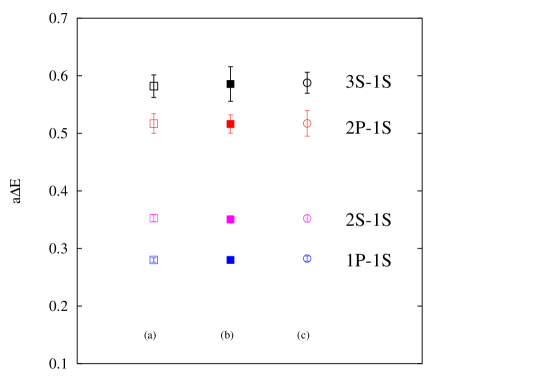
Figure 1: Dependence of $\Upsilon$ energy splittings on change in NRQCD stability parameter $n$ and choice of $u_{0}$: (a) $n=2$, $u_{0L}$ (b) $n=4$, $u_{0L}$ (c) $n=2$, $u_{0P}$. The results are from the 0.01/0.05 2+1 flavor coarse ensemble. $2S-1S$ etc indicates the splitting between radial excitations of the $\Upsilon$ and $1P-1S$ the splitting between the appropriate ${}^{1}P_{1}$ state and the $\Upsilon$.

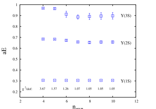
Figure 2: $\Upsilon$ energies in lattice units as a function of number of exponentials used in a $3\times 3$ matrix fit for results on the 0.01/0.05 coarse ensemble. $\chi^{2}/\mbox{dof}$ values indicate goodness of fit.

III Results

$0.0082/0.082$ $aE(1^{3}S_{1})$ 0.27755(36) $aE(2^{3}S_{1})$ 0.770(8) $aE(1^{1}P_{1})$ 0.6674(64)

Table 4: Fitted energies in lattice units for various radial and orbital excitations on the super-coarse ensemble.

$0.01/0.05$ $0.02/0.05$ $0.03/0.05$ $0.05/0.05$ 0.02 Quenched $aE(1^{3}S_{1})$ 0.30506(27) 0.30118(25) 0.29848(26) 0.29588(34) 0.29563(26) 0.26621(24) $aE(2^{3}S_{1})$ 0.6578(56) 0.6519(44) 0.627(10) 0.6381(95) 0.6326(79) 0.6073(49) $aE(3^{3}S_{1})$ 0.887(20) 0.878(22) 0.870(32) 0.927(21) 0.851(33) 0.887(12) $aE(1^{1}P_{1})$ 0.5852(37) 0.5705(41) 0.5593(70) 0.5593(61) 0.5519(59) 0.5111(27) $aE(2^{1}P_{1})$ 0.822(17) 0.801(16) 0.784(53) 0.827(18) 0.787(29) 0.788(12) $aE(1^{3}D_{2})$ 0.751(12) - - - - - $aE(2^{3}D_{2})$ 1.026(34) - - - - -

Table 5: Fitted energies in lattice units for different radial and orbital excitations for the coarse lattice ensembles.

$0.0062/0.031$ $0.0124/0.031$ Quenched $aE(1^{3}S_{1})$ 0.23248(46) 0.28677(40) 0.18517(23) $aE(2^{3}S_{1})$ 0.4818(33) 0.5303(27) 0.42734(25) $aE(3^{3}S_{1})$ 0.619(14) 0.671(13) 0.6472(71) $aE(1^{1}P_{1})$ 0.4233(37) 0.4705(30) 0.3595(19) $aE(2^{1}P_{1})$ 0.574(44) 0.628(16) 0.5470(86)

Table 6: Fitted energies in lattice units for various radial and orbital excitations on the fine lattice ensembles.

$n=4$ $u_{0}=\sqrt[4]{plaq}$ $aE(1^{3}S_{1})$ 0.29433(27) 0.47736(25) $aE(2^{3}S_{1})$ 0.6449(65) 0.8296(62) $aE(3^{3}S_{1})$ 0.8799(65) 1.0652(62) $aE(1^{1}P_{1})$ 0.5743(37) 0.7599(45) $aE(2^{1}P_{1})$ 0.811(16) 0.995(22)

Table 7: $\Upsilon$ spin independent energy splittings in lattice units on the coarse 2+1 flavor 0.01/0.05 ensemble. These were used for checking systematic errors by comparison with results in Table 5.

$3\times 3$ or $4\times 4$ matrix fits were performed to the $S$-wave correlators, and $2\times 2$ fits performed to the $P$- and $D$-wave correlators. $D$-wave correlators have only been calculated on the most chiral (0.01/0.05) 2+1 flavor coarse ensemble, and only for a subset of $D$-wave spin states. For each fit, the best $n_{exp}$ was chosen as one which gave a reasonable $\chi^{2}/\mbox{dof}$ and was large enough for fitted results to be independent of $n_{exp}$. The results for the fit energies are given in Tables 4, 5 and 6 for the super-coarse, coarse and fine lattices respectively. It is clear that the fitted energies are very accurate when compared to previous results, even from the quenched approximation scaling . This is partly because of the large number of configurations, their large physical volume and the large number of origins that we have been able to use. It is also partly because of the improved fitting strategy.

In the next two sections we will discuss the spin-independent aspects of the spectrum, that is the differences in mass between different radial and orbital excitations. In principle we should be using masses to calculate the mass splittings that are spin-averaged over the different spin states for each excitation. However, we cannot do that for the $S$-wave states since no ${}^{1}S_{0}$ state has been seen experimentally. For the $P$-wave states we can spin-average but it is easier to take simply the mass of the ${}^{1}P_{1}$ state. In potential models, where the spin-spin coupling induces a delta-function potential, the difference between the ${}^{1}P_{1}$ mass and that of the spin-average of the ${}^{3}P_{0,1,2}$ is expected to be zero. We will examine the limits to that assumption in section VII. In the meantime we will work with the ${}^{3}S_{1}$ and ${}^{1}P_{1}$ results from the Tables.

For completeness we also give the results for different values of stability parameter $n$ and tadpole-improvement factor $u_{0}$ for the 0.01/0.05 coarse ensemble in Table 7. It is clear from this table that, although changing $u_{0}$ does not affect spin-independent splittings, it does provide an overall shift to the energies.

IV Determining the lattice scale

$0.0082/0.082$ $a^{-1}_{2S-1S}$(GeV) 1.144(19)(11)(23) $a^{-1}_{1P-1S}$(GeV) 1.128(19)(28)(90)

Table 8: Inverse lattice spacing determinations for the super-coarse ensembles from both the $1^{1}P_{1}-1^{3}S_{1}$ and $2^{3}S_{1}-1^{3}S_{1}$ splittings. The first error given is statistical/fitting. The second is the expected systematic error from relativistic/radiative corrections and the third from discretisation errors.

$0.01/0.05$ $0.02/0.05$ $0.03/0.05$ $0.05/0.05$ 0.02 Quenched $a^{-1}_{2S-1S}$(GeV) 1.596(25)(11)(16) 1.605(20)(11)(16) 1.714(52)(12)(17) 1.645(46)(12)(16) 1.671(39)(12)(17) 1.651(24)(12)(17) $a^{-1}_{1P-1S}$(GeV) 1.571(21)(31)(63) 1.634(25)(33)(65) 1.687(45)(34)(67) 1.670(39)(33)(67) 1.717(40)(34)(68) 1.797(20)(36)(72)

Table 9: Inverse lattice spacing determinations for the coarse ensembles from both the $1^{1}P_{1}-1^{3}S_{1}$ and $2^{3}S_{1}-1^{3}S_{1}$ splittings. The first error given is statistical/fitting. The second is the expected systematic error from relativistic/radiative corrections and the third from discretisation errors.

$0.0062/0.031$ $0.0124/0.031$ Quenched $a^{-1}_{2S-1S}$(GeV) 2.258(30)(14)(9) 2.312(26)(14)(9) 2.324(24)(14)(9) $a^{-1}_{1P-1S}$(GeV) 2.305(45)(35)(35) 2.390(38)(36)(36) 2.524(28)(38)(38)

Table 10: Inverse lattice spacing determinations for the fine ensembles from both the $1^{1}P_{1}-1^{3}S_{1}$ and $2^{3}S_{1}-1^{3}S_{1}$ splittings. The first error given is statistical/fitting. The second is the expected systematic error from relativistic/radiative corrections and the third from discretisation errors.

The lattice spacing is fixed by the choice of $\beta$ but is not determined until after the simulation when a physical quantity is matched to experiment. Once the lattice spacing has been set in this way it can be used to give dimensionful predictions for other observables.

There should be only one value for the lattice spacing and therefore it should not matter which hadron mass or mass splitting is used in fixing it. However, it has been a long known problem that in fact this is not the case in lattice simulations with unrealistic (or completely missing) light-quark vacuum polarization. This is because different physical quantities probe different energy scales and the strong coupling constant will not run correctly between these scales unless the sea quark content (i.e. the quark vacuum polarization contribution) is sufficiently correct. This gives ambiguities in calculating physical observables as it is impossible to say what the ‘right’ lattice spacing is.

Determinations of the lattice spacing from different splittings can then be used as a guide to judge how physical is the sea quark content of the configurations being used. Here, the orbital $1P-1S$ (i.e. $1^{1}P_{1}-1^{3}S_{1}$) and radial $2S-1S$ (i.e. $2^{3}S_{1}-1^{3}S_{1}$) energy splittings independently fix the lattice spacing pdg . The results are given in Tables 8, 9 and 10 for the super-coarse, coarse and fine lattices respectively. There we list the statistical/fitting uncertainties in $a^{-1}$ and also give values for the expected systematic errors as estimated in Section II. The systematic errors will affect all the estimates of $a^{-1}$ in the same way, so it is only the differences between these errors that affect any discussion of differences between $a^{-1}$ determinations. We have not included an error from our inability to spin-average the $S$-wave states. The error from that is set by one quarter of the error in the spin-splitting (since we are using the vector state instead of the spin-average) and the spin-splitting is already only 10% of a typical spin-independent splitting. A 20% error in the spin-splitting from missing relativistic corrections would then lead to a 0.5% error in the determination of $a^{-1}$ from, for example, the $1P-1S$ splitting. This is negligible.

It is quite clear from these tables that there is a problem of internal consistency in the quenched approximation. The ratio of $a^{-1}$ from $1P-1S$ to that from $2S-1S$ is 1.09(2)(4) on the coarse quenched ensemble and 1.09(2)(1) on the fine quenched ensemble. The first error here is from statistics/fitting and the second from an estimate of the difference in systematic errors for the $1P-1S$ and $2S-1S$ splittings. Previous results from quenched NRQCD calculations also gave ratios larger than 1 further ; scaling ; sesam ; manke , although generally with lower significance because of poorer statistics or fitting. One problem with previous results was that most of them used an unimproved gluon action and the effect of the tree-level $\cal{O}$$(a^{2})$ discretisation errors is to reduce this ratio of $a^{-1}$ determinations by a few percent, obscuring the disagreement with 1. The ratio including a correction for this is given in reference scaling as 1.06(4) at $\beta$ = 6.0. Without correcting for it, reference sesam gives 1.12(9). It is clear that our new quenched results on improved glue are a considerable improvement in clarity on these previous results.

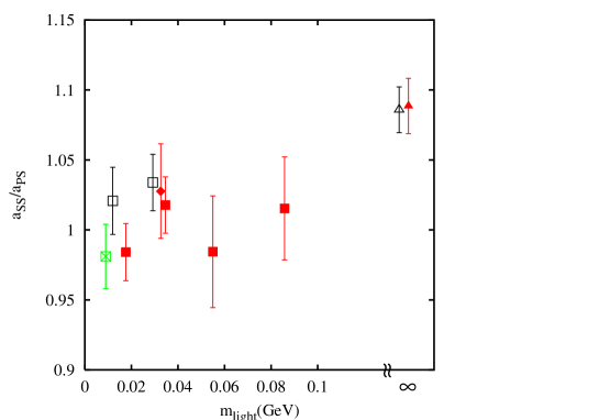
Figure 3: The ratio of lattice spacing values obtained from the $2S-1S$ and $1P-1S$ splittings in the $\Upsilon$ system as a function of bare light quark mass in the lattice QCD calculation. Notice the very magnified $y$-axis scale. The crossed square is from the super-coarse ensemble, the filled squares from the coarse 2+1 flavor ensembles and the open squares from the fine 2+1 flavor ensembles. The filled diamond is from the coarse $n_{f}=2$ ensemble. The open and filled triangles on the right of the plot are results from the quenched fine and coarse ensembles respectively. Errors are statistical only.

Figure 3 shows the ratio of lattice spacing determinations from the $2S-1S$ and $1P-1S$ splittings as a function of the bare light $(u/d)$ quark mass in our simulations (see Table 1). Also included are results with 2 flavors of sea quarks only, and over to the right of the plot, the quenched results. The ratio of inverse lattice spacings on the most chiral 2+1 flavor ensemble at each lattice spacing gives 0.981(23)(60) for super-coarse, 0.984(20)(34) for coarse and 1.021(23)(13) for fine, where the first error is statistical and the second systematic. All of these results are in agreement with 1, unlike the case in the quenched approximation. The results agree well with each other too, and this provides a check on our estimates of systematic errors from discretisation effects. For the fine lattices discretisation effects are small, but on the super-coarse lattices we have estimated that the $1P-1S$ splitting could be moved by 6% more than the $2S-1S$ splitting by discretisation and relativistic/radiative systematic errors. This looks like an overestimate since our super-coarse result agrees with 1 within statistical errors of 2%.

The agreement between the inverse lattice spacing results from the two different splittings is confirmation of the approach to the physical real world of a single inverse lattice spacing as the sea quark content is made realistic. Some signs of this were seen in earlier 2 flavor simulations upspaper ; further ; sesam ; marcantonio . Indeed here our 2 flavor results also give agreement with 1 for the ratio of lattice spacing values within the statistical error. As discussed earlier, the lattice spacing from the $2S-1S$ splitting is to be preferred on the grounds of systematic error and so we will use that in what follows.

We can also ask what the lattice spacing derived from $\Upsilon$ splittings implies for other quantities. A quantity that is used frequently to set the scale is the $r_{0}$ parameter sommer . It is derived from the heavy quark potential as the value of $r$ at which $r^{2}F(r)=1.65$, where $F(r)$ is the gradient of the potential. $r_{0}$ is easily and precisely calculable in lattice calculations but has the disadvantage that its value in physical units is not directly given by experiment. Instead its value must be given by numerical simulation on the lattice and comparison to an experimentally accessible quantity. Here we can give a value for $r_{0}$ from comparison to $\Upsilon$ splittings. In Figure 4 we plot $r_{0}$ in fm as a function of light sea quark mass, fixing the lattice spacing from the $2S-1S$ splitting. The value of $r_{0}$ in lattice units has been calculated by the MILC collaboration milc1 ; milc2 . The result does not show any dependence on either the light quark mass for light enough light quark mass or the lattice spacing. Our best result is from the fine lattices, and gives a physical value for $r_{0}$ equal to 0.469(7)fm. The error includes the systematic errors in the determination of the lattice spacing on the fine lattices and a similar systematic error for the determination of $r_{0}$. However these errors are small compared to the statistical error from the determination of the lattice spacing. This result is in agreement with the results from milc2 which were based on our preliminary analysis of the $\Upsilon$ results presented in this paper. We similarly have a value for the heavy quark potential variable $r_{1}$  milc2 (where $r^{2}F(r)=1.00$) of 0.321(5)fm. This is also shown as a function of light quark mass in Figure 5 and also agrees with the preliminary value from milc2 . This variable in fact shows a very flat curve as a function of light quark mass when the scale is set by the $\Upsilon$ $2S-1S$ splitting, i.e. the light quark vacuum polarisation effects are very similar in both variables. Note that if we had used the $1P-1S$ splitting to set the lattice spacing, both $r_{1}$ and $r_{0}$ would have had values in fm differing by 10% in the quenched approximation, because of the ambiguity in setting the lattice spacing demonstrated in Figure 3. The result on the chiral 2+1 flavor configurations would be unchanged, because here there is no ambiguity about the value of $a$ us .

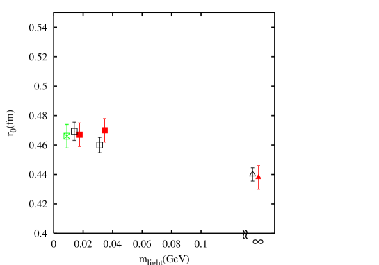
Figure 4: The value of $r_{0}$ in fm obtained on different super-coarse, coarse and fine ensembles, using the $2S-1S$ splitting in the $\Upsilon$ system to fix the lattice spacing. The crossed square is from the super-coarse ensemble, the filled squares from the coarse 2+1 flavor ensembles and the open squares from the fine 2+1 flavor ensembles. The open and filled triangles on the right of the plot are results from the quenched fine and coarse ensembles respectively. The $y$-axis scale is expanded to make error bars visible. $r_{0}$ values in lattice units are taken from milc1 ; milc2 ; milcprivate . Errors include the statistical errors from determining the lattice spacing and from determining $r_{0}$.

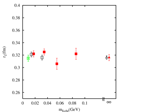
Figure 5: The value of $r_{1}$ in fm obtained on different super-coarse, coarse and fine ensembles, using the $2S-1S$ splitting in the $\Upsilon$ system to fix the lattice spacing. The crossed square is from the super-coarse ensemble, the filled squares from the coarse 2+1 flavor ensembles and the open squares from the fine 2+1 flavor ensembles. The open and filled triangles on the right of the plot are results from the quenched fine and coarse ensembles respectively. The $y$-axis scale is expanded to make error bars visible. $r_{1}$ values in lattice units are taken from milc1 ; milc2 ; milcprivate . Errors include the statistical errors from determining the lattice spacing and from determining $r_{1}$.

V Comparing radial and orbital splittings to experiment

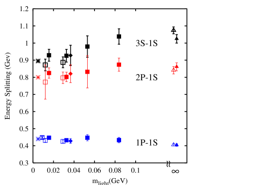
Figure 6: Spin-independent splittings in the $\Upsilon$ spectrum as a function of bare sea light quark mass. The $1P-1S$, $2P-1S$, and $3S-1S$ splittings are shown. The $S$ state is always the ${}^{3}S_{1}$. The $P$ state from the lattice calculations is the ${}^{1}P_{1}$; from experiment it is the spin-average of ${}^{3}P_{0,1,2}$. Closed squares are from coarse 2+1 flavor lattices and open squares from fine 2+1 flavor lattices. The crossed square for the $1P-1S$ splitting is from the super-coarse ensemble. Closed diamonds are from the coarse $n_{f}=2$ run. Closed and open triangles are from quenched coarse and fine ensembles respectively. Bursts give the experimental results. Errors include the statistical errors from determining the lattice spacing from the $2S-1S$ splitting.

The $2S-1S$ inverse lattice spacing values and fit energies from the previous sections were combined to give dimensionful determinations of the radial and orbital splittings $3^{3}S_{1}-1^{3}S_{1}$, $1^{1}P_{1}-1^{3}S_{1}$, $2^{1}P_{1}-1^{3}S_{1}$. Figure 6 plots the results as a function of the sea light quark mass for the coarse and fine ensembles. Bursts denote the experimental values where we have used the spin-average of the $\chi_{b}$ states in place of the unobserved $h_{b}$.

Good agreement with experiment is seen as the chiral limit is approached and the flatness of the approach indicates that chiral extrapolations would have no significant effect in shifting the results from the most chiral ensemble.

Figure 7 shows the radial and orbital levels in the $\Upsilon$ spectrum with the lattice results from the coarse and fine 2+1 flavor ensembles with lightest sea quark mass contrasted to coarse and fine quenched results. The solid lines are the experimental values, including the recently observed ${}^{3}D_{2}$ state cleo . On the lattice the spin 2 representation is split into two representations labelled $E$ and $T$. Here we used the $E$ representation. This will be discussed further in section VII. The $1S$ energy and $2S-1S$ splitting are not predictions as they have already been used to fix the $b$ quark mass in lattice units and the lattice spacing respectively. The quenched results clearly do not agree with experiment for other splittings whereas the 2+1 flavor results do.

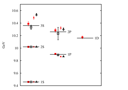
Figure 7: The $\Upsilon$ spectrum of radial and orbital levels, taking the most chiral points from Figure 6. Closed and open symbols are from coarse and fine lattices respectively. Squares and triangles denote unquenched and quenched results respectively. Lines represent experiment.

VI The $b$ quark mass

The bare $b$ quark mass in the lattice Lagrangian is fixed by the requirement to get the $\Upsilon$ mass correct. Because the quark mass term has been removed from the NRQCD Lagrangian the energies calculated for hadrons at zero momentum are shifted from their masses. This means that energy differences (for particles containing the same number of quarks or antiquarks) do give mass differences but in order to fix one mass absolutely, a dispersion relation must be calculated. In sections IV and V we discussed energy differences and mass splittings. Here we give results for the mass of the $\Upsilon$ from calculations of its energy as a function of lattice momentum, and discuss how well the $b$ quark mass can then be determined.

VI.1 Fixing the $\Upsilon$ mass

The continuum relationship between energy, $E$, and spatial momentum, $\vec{p}$, for a hadron in a theory such as NRQCD where the zero of energy has been shifted is given by:

$$E(p)=E(0)+\sqrt{p^{2}+M^{2}}-M.$$ (9)

The hadron mass is denoted by $M$ here, sometimes called the kinetic mass to emphasise that it is determined from a dispersion relation rather than $E(0)$. Equation 9 is a fully relativistic formula. When used in our lattice calculations, $\vec{p}$ is a lattice momentum given in lattice units by $2\pi(n_{x},n_{y},n_{z})/L$ where $L$ is the number of lattice spacings in the spatial directions (16 for super-coarse, 20 for coarse and 28 for fine) and $n_{x,y,z}$ take integer values between 0 and $L-1$. $M_{kin}$ is obtained by first fitting the energy of jack-knifed ratios of $\Upsilon$ correlators at zero and non-zero values of $p$ to an exponential form. The exponent yields the energy difference $\Delta E=E(p)-E(0)$ and

$$M=\frac{p^{2}-(\Delta E)^{2}}{2\Delta E}.$$ (10)

Note that a non-relativistic formula would not include the $(\Delta E)^{2}$ term, and this becomes increasingly negligible as the mass increases.

$n^{2}$ $a\Delta E$ $aM_{\Upsilon}$ $c^{2}$ 1 0.008264(40) 5.967(29) - 2 0.016507(84) 5.971(30) 0.999(5) 3 0.02473(13) 5.974(32) 0.999(5) 4 0.03286(19) 5.990(34) 0.996(6) 5 0.04104(25) 5.991(36) 0.996(6) 6 0.04928(31) 5.983(37) 0.997(6) 8 0.06540(47) 6.004(43) 0.994(7) 9 0.07353(57) 6.003(46) 0.994(8) 12 0.09778(92) 6.007(56) 0.993(9)

Table 11: Energy differences of zero and non-zero momentum $\Upsilon$ mesons, and resulting $\Upsilon$ masses, in lattice units. Non-zero momenta are denoted by $n^{2}=n_{x}^{2}+n_{y}^{2}+n_{z}^{2}$. These are unambiguous except for $n^{2}=9$ which corresponds to the $n$-vector (2,2,1) and its permutations. The fourth column gives values for the speed of light, $c^{2}$, defined in the text. The results are for the coarse 2+1 flavor 0.01/0.05 ensemble.

Table 11 gives, as an example of our results, values for $\Delta E$ and $M$ obtained on the coarse $2+1$ flavor 0.01/0.05 ensemble for a range of lattice momenta. These results are plotted in physical units (using the lattice spacing from the $2S-1S$ splitting of section IV) in Figure 8. Figure 8 shows that the $\Upsilon$ mass is stable and well-determined out to very large values of $p^{2}$, far larger than are routinely accessible in light hadron calculations. The value does not change significantly, showing that lattice artefact terms and errors coming from missing relativistic corrections to the NRQCD action in the lattice dispersion relation are not significant.

An equivalent illustration of the stability of the $\Upsilon$ mass is given by the ratio of the $p$ and $E$ terms in Equation 9. This ratio is called the ‘speed of light’ and should have value 1 in our units. We calculate it as:

$$c^{2}=\frac{(\Delta E)^{2}+2M\Delta E}{p^{2}}.$$ (11)

where $M$ is determined from above using values of $p$ corresponding to $n^{2}$ = 0 and 1. This is a quantity much used as a check of how well discretisation errors are controlled in actions for light quarks on the lattice klassenalford . Even the best light quark actions show discrepancies of $c^{2}$ from 1 of a few percent at typical lattice spacing values; some of the poorer actions show discrepancies of many percent kayaba . Our results are tabulated in Table 11 and plotted in Figure 9. They show that $c^{2}$ never deviates from 1 by as much as 1% and we can determine it with errors of less than 1%.

Deviations from 1 of $c^{2}$ would be caused by both missing higher order relativistic corrections in the NRQCD action and discretisation errors in the NRQCD and gluon actions. The terms that give rise to these errors have been discussed in Section II. Here we can estimate their effect on $c^{2}$ by assuming that the momentum of the $\Upsilon$ is shared between the two quarks equally. The relative error in $\Delta E$ from missing radiative corrections to the $(\Delta^{(2)})^{2}$ relativistic correction in Equation 1 is then $\alpha_{s}(p/2)^{2}/(2M_{b}^{0})^{2}$. This only amounts to 0.5% even at momentum $(2,2,2)$ on the coarse set of ensembles, and 0.4% on the fine set. Similarly missing radiative corrections to the discretisation errors, i.e. the effect of setting $c_{5}$ and $c_{6}$ to 1, amount to no more than 0.5% at momentum $(2,2,2)$ on the coarse set of ensembles, 1% on the super-coarse set and 0.2% on the fine set. These estimates bear out the results shown in Figure 9 and emphasise how well the NRQCD formalism handles heavy quarks at low non-zero momenta. This is important not only for extracting hadron masses but also for the analysis of form factors for $B$ meson semi-leptonic decay junko .

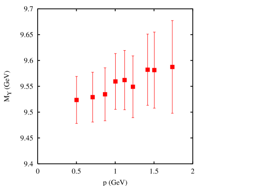
Figure 8: The value of the $\Upsilon$ mass in physical units plotted against the the lattice momentum for the $n_{f}=2+1$ 0.01/0.05 coarse ensemble for $aM^{0}_{b}=2.8$. Errors included are only those from determining $M_{\Upsilon}$, since the errors from determining the lattice spacing are the same for all points.

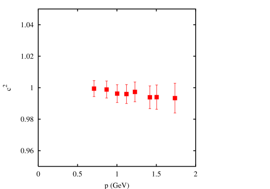
Figure 9: The ‘square of the speed of light’ (see text for definition) from $\Upsilon$ correlators at non-zero momentum for the $n_{f}=2+1$ 0.01/0.05 coarse ensemble and $aM^{0}_{b}=2.8$. Note the large magnification of the $y$-axis scale to make the errors visible.

We obtain values for the $\Upsilon$ mass from Equation 10 using momenta 0 and $n^{2}=1$. These are given in Tables 12, 13, 14 for our super-coarse, coarse and fine ensembles respectively.

$0.0082/0.082$ $aM_{\Upsilon}$ 8.086(17) $M_{\Upsilon}$/GeV 9.25(15)(21)

Table 12: The $\Upsilon$ mass in lattice units and physical units obtained from momenta 0 and $n^{2}=1$ for the super-coarse ensemble. The results in lattice units include statistical/fitting errors only; the results in physical units include two errors. The first is statistical/fitting, dominated by that from determining the lattice spacing from the $2S-1S$ splitting. The second error is the combined systematic error from the lattice spacing determination.

$0.01/0.05$ $0.02/0.05$ $0.03/0.05$ $0.05/0.05$ 0.02 Quenched $aM_{\Upsilon}$ 5.968(29) 5.942(29) 5.935(26) 5.906(34) 5.875(27) 5.855(37) $M_{\Upsilon}$/GeV 9.52(16)(11) 9.54(13)(11) 10.17(31)(12) 9.72(28)(11) 9.82(23)(11) 9.67(15)(11)

Table 13: The $\Upsilon$ mass in lattice units and physical units obtained from momenta 0 and $n^{2}=1$ for the coarse set of ensembles. The results in lattice units include statistical/fitting errors only; the results in physical units include two errors. The first is statistical/fitting, dominated by that from determining the lattice spacing from the $2S-1S$ splitting. The second error is the combined systematic error from the lattice spacing determination.

$0.0062/0.031$ $0.0124/0.031$ Quenched $aM_{\Upsilon}$ 4.218(18) 4.268(15) 4.145(12) $M_{\Upsilon}$/GeV 9.52(13)(7) 9.87(12)(7) 9.63(10)(7)

Table 14: The $\Upsilon$ mass in lattice units and physical units obtained from momenta 0 and $n^{2}=1$ for the fine set of ensembles. The results in lattice units include statistical/fitting errors only; the results in physical units include two errors. The first is statistical/fitting, dominated by that from determining the lattice spacing from the $2S-1S$ splitting. The second error is the combined systematic error from the lattice spacing determination.

VI.2 Determining the $b$ quark mass

The bare $b$ mass. The values for the $\Upsilon$ masses are in agreement with the experimental $\Upsilon$ mass for most of our ensembles, indicating that the bare quark masses used for the $b$ quarks are good ones. There is particularly close agreement for the most important ensembles - the most chiral coarse and fine unquenched ensembles. Because the calculated $\Upsilon$ mass in physical units is proportional to a good approximation to the bare quark mass in physical units, shifts of the bare lattice quark mass and shifts of the lattice spacing compensate each other mb when calculating the bare quark mass in physical units. This means that errors in the lattice spacing determination or in the tuning of the bare quark mass in lattice units do not in fact feed through into errors in the bare quark mass in GeV. This is demonstrated most clearly if we determine

$$\mbox{$M_{b}^{0}$}(a)=a\mbox{$M_{b}^{0}$}_{sim}\frac{M_{\Upsilon,expt}}{aM_{\Upsilon,latt}}$$ (12)

where $a\mbox{$M_{b}^{0}$}_{sim}$ is the bare lattice $b$ quark mass in lattice units used in the calculation (see Table 1). We tabulate the values of $\mbox{$M_{b}^{0}$}(a)$ from this formula for each of our lattice spacings in Table 15. The errors quoted include statistical errors (which range from 0.2% to 0.5%) as well as systematic errors from relativistic/discretization errors. The latter are estimated by noting that the binding energy is only 6% of the $\Upsilon$ mass (as we shall see below). The leading errors, from missing radiative corrections to the leading relativistic/discretization corrections, are expected to be 20-30% of that 6%. Note that the bare mass, $\mbox{$M_{b}^{0}$}(a)$, decreases with decreasing lattice spacing, as expected for a running mass. The masses from the comparable quenched simulations are only slightly higher at 4.52 GeV on the coarse ensemble and 4.45 GeV on the fine ensemble. We now discuss the conversion of the bare mass first to a perturbative pole mass and then to an $\overline{MS}$ mass for the $b$ quark.

Renormalization of the $b$ quark mass. There are two methods for determining the $b$ pole mass, defined perturbatively, from an NRQCD simulation mb . Both use perturbative results obtained from the heavy quark self-energy gulez . The first uses perturbation theory to relate the pole mass directly to $\mbox{$M_{b}^{0}$}(a)$, defined above:

$$M_{b}^{\mathrm{pole}}=Z_{m}\,M_{b}^{0}\equiv\left(1+C_{M}\,\alpha_{s}+\cdots\right)\,M_{b}^{0}$$ (13)

where $C_{M}$ depends on $a\mbox{$M_{b}^{0}$}$ and values are given in Table 15 gulez . The second method uses perturbation theory to relate the NRQCD energy of the $\Upsilon$ to the ‘binding energy’ of the meson and therefore to the pole mass:

$$M_{b}^{pole}=\frac{1}{2}(M_{\Upsilon,expt}-(E_{sim}-2E_{0}))$$ (14)

where $E_{sim}$ is the fitted NRQCD energy from $\Upsilon$ correlators at zero momentum given in Tables 4, 5, 6. Here $E_{0}$ is the NRQCD energy of an isolated $b$ quark, computed in perturbation theory:

$$aE_{0}=C_{E_{0}}\alpha_{s}+\cdots.$$ (15)

$C_{E_{0}}$ again depends upon $aM_{b}^{0}$ and the appropriate values are given in Table 15).

Unfortunately the momentum scales for $\alpha_{s}$ in our two perturbative formulas are quite small. Working in the $V$ scheme and using BLM scale fixing blm ; tadimp an earlier analysis, using a slightly different version of NRQCD and an unimproved gluon action, found scales of order $0.6/a$ for both the $Z_{m}$ and $aE_{0}$ expansions colin2 . Even on our finest lattices, $\alpha_{V}(0.6/a)$ is about 0.75 quentin . The small scale is expected. It reflects real infrared sensitivity in the pole mass. Such large values for the coupling constant mean that we cannot obtain an accurate estimate of the pole mass.

$M_{b}^{0}$/GeV $C_{M}$ $C_{E_{0}}$ $M_{b}^{\overline{MS}}(M_{b}^{\overline{MS}})$/GeV super-coarse 4.68(9) 0.082 0.850 4.31(44) coarse 4.44(7) 0.235 0.767 4.30(31) fine 4.37(5) 0.421 0.689 4.44(26)

Table 15: The $b$ quark mass in physical units from the most chiral 2+1 flavor lattice ensembles (i.e. 0.0082/0.082 super-coarse, 0.01/0.05 coarse and 0.0062/0.031 fine). The bare mass is given on the left, the perturbative coefficients in $Z_{m}$ and $E_{0}$ (see text) in the centre and the mass in the $\overline{MS}$ scheme at its own scale on the right. For the bare mass the error is dominated by a systematic error from the NRQCD action; for the $\overline{MS}$ mass the error is an estimate from unknown higher orders in perturbation theory.

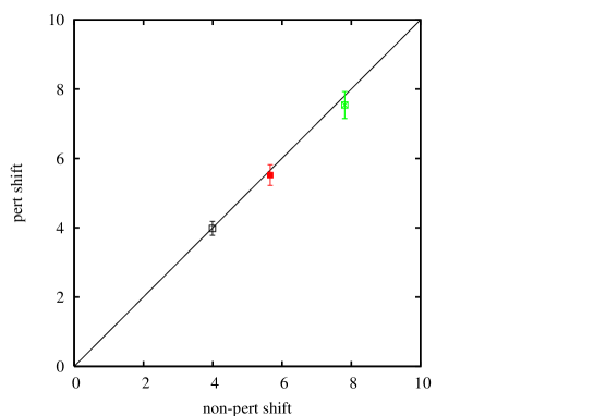
Figure 10: The perturbative estimate of the shift between mass and simulation energy for the $\Upsilon$ versus the result obtained non-perturbatively from our calculations. The results are given in lattice units for the most chiral 2+1 flavor ensembles on super-coarse (0.0082/0.082), coarse (0.01/0.05) and fine (0.0062/0.031) lattices (right to left). The errors on the perturbative points are estimates of unknown $\alpha_{s}^{2}$ terms, taken as $2\times\alpha_{V}^{2}(q*)$ for 2 $b$ quarks in an $\Upsilon$; the errors on the non-perturbative results are negligible in comparison (0.5%). The line drawn is $y=x$ for comparison.

By equating our two formulas for $M_{b}^{\mathrm{pole}}$, we obtain an interesting relationship between $b$ quark and $\Upsilon$-meson properties:

$$2(Z_{M}M_{b}^{0}-E_{0})=M_{\Upsilon}-E_{\mathrm{sim}}$$ (16)

The quantities on the right-hand side of this equation are measured nonperturbatively in our simulations, while the left-hand side is determined from perturbation theory. The infrared sensitivity that plagues the pole mass cancels between the two terms on the right-hand side, so that scales $q^{*}$ for $\alpha_{V}$ vary from approximately 1.7/a to 1.3/a from super-coarse to fine lattice spacings colinpriv . We compare the perturbative predictions (left-hand side) and our nonperturbative measurements (right-hand side) for this shift in Figure 10. The agreement is excellent even as this shift varies by almost a factor of two.

The $\overline{MS}$ $b$ quark mass. Our inability to obtain a pole mass is not much of a handicap since most applications require the $\overline{\mathrm{MS}}$ mass. The $\overline{\mathrm{MS}}$ mass, like $M_{b}^{0}$, is a bare mass, and therefore is free of the infrared problems associated with the pole mass. We can convert our previous formulas for $M_{b}^{\mathrm{pole}}$ into formulas for $M_{b}^{\overline{\mathrm{MS}}}$ using the standard formula,

$$M_{b}^{\overline{\mathrm{MS}}}(\mu)=\left(1-\frac{\alpha_{s}}{\pi}\,(\frac{4}{3}+2\log(\frac{\mu}{M_{b}})+\cdots\right)\,M_{b}^{\mathrm{pole}}.$$ (17)

Combining this formula with Equation 13 gives

$$M_{b}^{\overline{\mathrm{MS}}}(\mu)=\left(1+\frac{\alpha_{s}}{\pi}\,(C_{M}\pi-\frac{4}{3}-2\log(\frac{\mu}{M_{b}^{0}}))+\cdots\right)\,M_{b}^{0}.$$ (18)

The choice of the $\overline{\mathrm{MS}}$ scale $\mu$ is arbitrary, but we want to choose a scale that matches the $\overline{\mathrm{MS}}$ and lattice cutoffs — so that the two bare masses, $M_{b}^{\overline{\mathrm{MS}}}(\mu)$ and $M_{b}^{0}$, are roughly equivalent. An obvious choice is the scale $\mu^{*}$ such that the first-order coefficient in Equation 18 vanishes; this gives values for $a\mu*$ between 2.4 and 1.9 for our three lattice spacings, showing only weak $a$-dependence (as expected when $aM_{b}\gg 1$). We simplify the analysis here by setting $\mu=2/a$ for all of our lattice spacings, resulting in first-order coefficients that range from 0.16 to 0.06. Previous work kent2 suggests that an appropriate coupling constant in this formula is $\alpha_{V}(2/a)$, where, as expected, the scale is much larger than for the pole-mass formulas. We again take values for $\alpha_{V}$ from quentin . Our final results, evolved to the $\overline{\mathrm{MS}}$ mass using 3-loop evolution melnikov , are quoted in Table 15. These include a perturbative error uncertainty which we estimate to be $1\times\alpha_{V}^{2}(2/a)$. Our results from different lattice spacings are in excellent agreement; we take 4.4(3) GeV as our final result.

Further checks of the $b$ quark mass. An important check of the $b$ quark mass is whether the masses of other hadrons containing $b$ quarks calculated on the lattice agree with experiment when the $b$ quark mass is fixed from the $\Upsilon$ mass. In the quenched approximation this has always been problematic as a result of the ambiguity in determination of the lattice spacing. This led to large differences in $b$ quark masses used in $B$ calculations and $\Upsilon$ calculations - 30% at $\beta$=6.0 upspaper ; arifa . In a lattice simulation which matches the real world there is only one value for the lattice spacing and one value for the bare $b$ quark mass. Here we test this for the MILC 2+1 flavor configurations.

Figure 11 gives the mass for the $B_{s}$ meson on the 2+1 flavor 0.01/0.05 coarse ensemble using a bare $b$ quark mass that is the same as that of the $\Upsilon$ calculation and fixing the lattice spacing from the $2S-1S$ $\Upsilon$ splitting, again as in the $\Upsilon$ calculation. The $B_{s}$ mass is obtained from the dispersion relation, Equation 9, as for the $\Upsilon$. The $s$ quark mass is fixed from the $K$ mass ourms . The experimental $B_{s}$ mass is 5.37 GeV so the lattice results are 4% or 1$\sigma$ high, i.e. in agreement within errors. This is a big improvement over the results in the quenched approximation and shows that these unquenched configurations are at last yielding an unambiguous picture of the real world.

There is a potential systematic error of 1-2%, as explained above, coming from the NRQCD action in the $\Upsilon$ case. As we now explain, this source of error is not mirrored in the $B$ system, and so does remain a potential systematic difference between the two. This can certainly explain the results in Figure 11 if they are not simply statistical fluctuation, and would indicate that further improvements to the NRQCD action would remove any discrepancy.

The power-counting for the NRQCD action for a heavy-light meson is quite different from that of a heavy-heavy meson, since it is then powers of $1/M_{b}$ that matter, with $\Lambda_{QCD}/M_{b}\approx$ 10% for the $B$. All terms through second-order ($1/M_{b}^{2}$) are included at tree-level in the NRQCD action we have used, Equation 1, and we expect smaller systematic errors than in $\Upsilon$ system. Formally the largest systematic error comes from radiative corrections to the $\vec{\sigma}\cdot\vec{B}/M_{b}$ term but this term itself does not have a large effect as can be seen from comparing the $B$ meson hyperfine splitting to the $B$ mass. The $B$ meson binding energy ($E_{sim}-E_{0}$) is quite a different size, and of different sign, to that of the $\Upsilon$. It arises largely from the light quark sector and here errors from the improved staggered action appear. These are formally $\alpha_{s}(a\Lambda_{QCD})^{2}$ which can be estimated to be around 2%, but applied to the binding energy this gives a very small error in the $B$ meson mass.

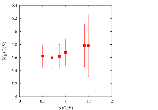
Figure 11: The value of the $B_{s}$ mass in physical units plotted against the lattice momentum for the $n_{f}=2+1$ 0.01/0.05 coarse ensemble for $aM^{0}_{b}=2.8$, and $am_{s}=0.04$ using the MILC convention for light quark mass. Errors included are only those from determining $M_{kin}$, since the errors from determining the scale are the same for all points.

Another check of agreement with experiment with unquenched lattice QCD is to study $2m_{B}-m_{\Upsilon}$ or $2m_{B_{s}}-m_{\Upsilon}$. Explicit terms in the $b$ quark mass cancel in this difference leaving sensitivity to the differences in binding energies in the two systems (with slight heavy quark mass dependence). From the discussion above we expect systematic errors of order 2% in this quantity, coming either from errors in the NRQCD action on the heavy-heavy side or from discretisation errors in the light quark action on the heavy-light side. To avoid errors on the heavy-light side coming from radiative corrections to the $\vec{\sigma}\cdot\vec{B}$ term, we spin-average over pseudoscalar and vector heavy-light states. The results are shown in Figure 12 and show indeed good agreement with the experimental results at the level expected. This is again strong confirmation that lattice QCD with light sea quarks reproduces experimental hadron masses across a wide range of the spectrum.

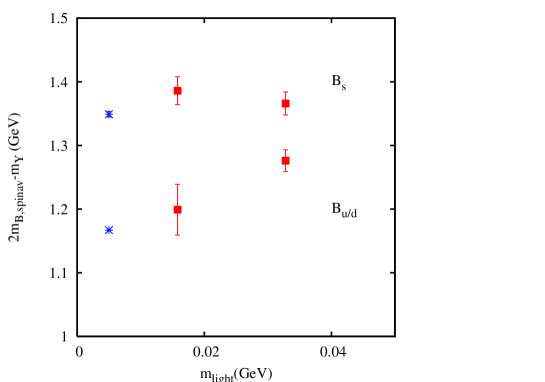
Figure 12: The mass difference between twice the spin-average of $B$ and $B^{*}$ and the $\Upsilon$ for $B_{u/d}$ and $B_{s}$, plotted against the sea $u/d$ mass in physical units for coarse unquenched configurations. The results are for the 2+1 flavor 0.01/0.05 and 0.02/0.05 lattices. The $u/d$ mass used in the $B_{u/d}$ is then 0.01 or 0.02 as appropriate and the $s$ mass used in the $B_{s}$ is 0.04, fixed from the $K$ mass ourms . The upper points are for the $B_{s}$ and the lower for the $B_{u/d}$. The experimental results are given by the bursts pdg where we have assumed that the $B^{*}_{s}$-$B_{s}$ splitting is the same as that for the $B_{u/d}^{*}$-$B_{u/d}$. Errors include statistics/fitting and $a^{-1}$ errors.

VII Fine structure in the $\Upsilon$ spectrum

$0.0082/0.082$ $aE(1^{3}S_{1})-aE(1^{1}S_{0})$ 0.0348(5) $aE(2^{3}S_{1})-aE(2^{1}S_{0})$ 0.018(13) $\frac{E(2^{3}S_{1})-E(2^{1}S_{0})}{E(1^{3}S_{1})-E(1^{1}S_{0})}$ 0.52(38)

Table 16: $S$-wave fine structure in the $\Upsilon$ spectrum for the super-coarse 2+1 flavor lattice ensemble. Energies are given in lattice units. Errors are statistical/fitting only.

$0.01/0.05$ $0.02/0.05$ $0.03/0.05$ $0.05/0.05$ 0.02 Quenched $aE(1^{3}S_{1})-aE(1^{1}S_{0})$ 0.03128(34) 0.03062(32) 0.02972(33) 0.02925(43) 0.02668(34) 0.02152(30) $aE(2^{3}S_{1})-aE(2^{1}S_{0})$ 0.0111(75) 0.0172(62) 0.017(14) 0.013(13) 0.0102(109) 0.0137(78) $\frac{E(2^{3}S_{1})-E(2^{1}S_{0})}{E(1^{3}S_{1})-E(1^{1}S_{0})}$ 0.35(24) 0.56(20) 0.57(47) 0.44(44) 0.38(41) 0.64(36)

Table 17: $S$-wave fine structure in the $\Upsilon$ spectrum for the coarse ensembles. Energies are given in lattice units. Errors are statistical/fitting only.

$0.0062/0.031$ $0.0124/0.031$ Quenched $aE(1^{3}S_{1})-aE(1^{1}S_{0})$ 0.02599(53) 0.02422(45) 0.01735(29) $aE(2^{3}S_{1})-aE(2^{1}S_{0})$ 0.0141(55) 0.0120(42) 0.0107(31) $\frac{E(2^{3}S_{1})-E(2^{1}S_{0})}{E(1^{3}S_{1})-E(1^{1}S_{0})}$ 0.54(21) 0.50(18) 0.62(18)

Table 18: $S$-wave fine structure in the $\Upsilon$ spectrum for the fine lattice ensembles. Energies are given in lattice units. Errors are statistical/fitting only.

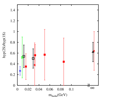
Figure 13: The ratio of the splitting between the $\Upsilon^{\prime}$ and $\eta^{\prime}_{b}$ to that between the $\Upsilon$ and the $\eta_{b}$. Crossed squares are from super-coarse lattices, closed squares are from coarse lattices and open squares from fine lattices. The closed diamond is from the coarse $n_{f}=2$ ensemble. The closed and open triangles are from the coarse and fine quenched ensembles. The burst represents the current experimental result for the $\psi$ system, using the value for the mass of the $\eta_{c}^{\prime}$ from the BELLE collaboration belle .

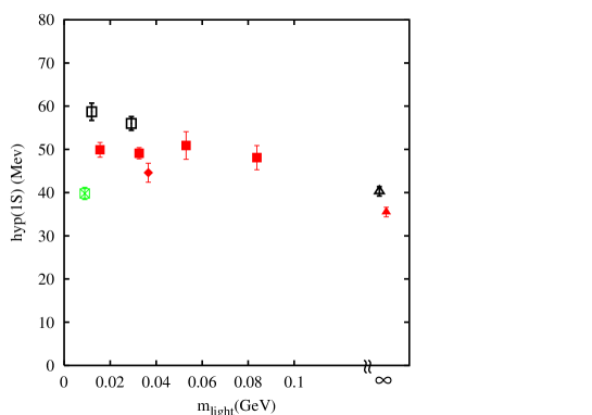
Figure 14: The ground-state hyperfine splitting in the $\Upsilon$ system as a function of the light quark mass included in the quark vacuum polarization. Crossed, closed and open symbols are from super-coarse, coarse and fine lattices respectively. Squares and triangles denote unquenched and quenched results respectively. The closed diamond is from the coarse $n_{f}=2$ ensemble. Errors include both statistical/fitting errors from determining the splitting and from determining the lattice spacing scale. This latter error appears doubled (see text). Note that there is an additional overall systematic error of 25% discussed in the text.

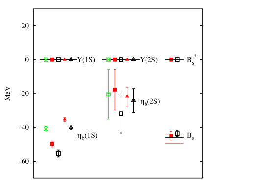
Figure 15: Hyperfine splittings in the $\Upsilon$ and $B_{s}$ systems. Crossed, closed and open symbols are from super-coarse, coarse and fine lattices respectively. Squares and triangles denote unquenched and quenched results respectively. The unquenched results are from the ensembles in Table 1 that include the lightest light quark mass in the quark vacuum polarization at each value of the lattice spacing. Errors include both statistical/fitting errors from determining the splitting and from determining the lattice spacing scale as in Figure 14. Additional systematic errors are 25% and discussed in the text. The unquenched results include a renormalisation to the correct value for $u_{0L}$ (see text). The faint lines give the experimental limits on the $B_{s}^{*}-B_{s}$ splitting and the dark line gives the experimental result for $B^{*}-B$ pdg .

Fine structure in the $\Upsilon$ spectrum arises from terms in the action which are suppressed by a power of $v^{2}$ compared to the leading term, $H_{0}$. Such sub-leading terms themselves have sub-leading corrections which we have not included. We expect therefore that the results we obtain are only accurate to $\cal{O}$$(v^{2})=10\%$. In addition there are $\cal{O}$$(\alpha_{s})$ corrections to the coefficients of these terms, such as $c_{4}$ in equation 1, which could amount to a 20-30% error. In fact, as we shall see, we are able to do rather better than this, but results in this section are still rather qualitative. We present them nevertheless as providing useful pointers for future calculations.

VII.1 $S$-wave fine structure

There are no experimental results for either the ground or radially excited $S$-wave spin splitting (hyperfine splitting) in the $\Upsilon$ system, and so these are key results to be predicted by lattice QCD. This splitting is the mass difference between the vector ($\Upsilon$) state and the pseudoscalar ($\eta_{b}$) and so a prediction of the splitting is equivalent to a prediction of the unknown $\eta_{b}^{(\prime)}$ mass. Our result for the ground-state hyperfine splitting is 61(14) MeV, giving $M_{\eta_{b}}$ = 9.399(14) GeV. Our prediction for the radially excited hyperfine splitting is 30(19) MeV, giving $M_{\eta_{b}^{\prime}}$ = 9.993(19) GeV. The largest contribution to the error for the ground-state splitting comes from unknown radiative corrections to the spin-dependent term in the NRQCD action that gives rise to this splitting. For the excited state splitting the dominant error is statistical. How we estimate the size of the errors and how we can reduce them in future is described in more detail below.

Results for the ground and radially excited hyperfine splitting in lattice units, and their ratio are given in Tables 16, 17 and 18 for the super-coarse, coarse and fine MILC lattices respectively. Splittings are obtained from the difference in fitted energies of the ${}^{3}S_{1}$ ($\Upsilon$) and ${}^{1}S_{0}$ ($\eta_{b}$) states using $3\times 3$ fits ($2\times 2$ fits on the super-coarse lattices). Bootstrapping the fits together improved the errors in some cases, and not in others, and so we do not give bootstrap errors here. The results for the hyperfine splitting are very precise because it is the difference between two ground $S$-wave states which are very well-determined. This means that statistical errors are small and differences between different lattice calculations show up clearly. The possibility of significant systematic errors in the splitting, however, must not be forgotten.

Figure 13 shows the ratio of the hyperfine splitting for the 1st radial excitation to that of the ground state i.e. $(M_{\Upsilon^{\prime}}-M_{\eta_{b}^{\prime}})/(M_{\Upsilon}-M_{\eta_{b}})$. The hyperfine splitting is controlled by the ${\bf\sigma}\cdot{\bf B}$ term in the NRQCD action and is then proportional to the square of $c_{4}$ (see Equation 1). $c_{4}$ cancels in the ratio so in principle it can be accurately determined in our lattice calculation with $c_{4}$ set to 1. The statistical errors here are large but we obtain a result of 0.5(3). There is no sign of significant dependence on the lattice spacing or on the light quark mass. The result is in keeping with the experimental results in the charmonium system, plotted as a burst in the Figure belle . The charmonium result is not irrelevant because we also expect a lot of the heavy quark mass dependence to cancel in the ratio of splittings.

Figure 14 shows our results for the ground-state hyperfine splitting in MeV as a function of the bare quark mass of the light quarks included in the quark vacuum polarisation. We use the lattice spacing values from the $2S-1S$ splitting of Section IV to convert to physical units. Results are shown for the super-coarse, coarse and fine ensembles. The errors on the points include the very small statistical error from the splitting itself and also the much larger error from the uncertainty in the lattice spacing. This uncertainty in fact appears multiplied by two because the hyperfine splitting is approximately inversely proportional to the physical quark mass. Any underestimate of the inverse lattice spacing will both reduce the hyperfine splitting directly and also reduce it indirectly by reducing the quark mass scaling , so that the splitting must then be readjusted downwards to correspond to the correct meson mass. We then have a statistical/fitting error of 5% on the ground-state hyperfine splitting in physical units.

The results show significant dependence on both the lattice spacing (to be discussed further below) and the number of flavors of quark, $n_{f}$, included in the quark vacuum polarisation at a given lattice spacing. Neither of these points is surprising. In the language of a simple potential model the hyperfine splitting arises from a very short-range spin-spin potential, dominated by the perturbative contribution which is a delta function at the origin. We therefore expect sensitivity to the lattice spacing scaling and also to the value of $\alpha_{s}$ at short distance, which depends strongly on $n_{f}$ quentin . The results do not however, show significant dependence on the bare light quark mass. This is also not surprising, as for spin-independent splittings, because of the large gluon momenta involved. Provided that the light quark mass is light enough, as is the case here, the splitting simply ‘counts’ the number of light quark flavors. We do not therefore attempt any extrapolation in the light quark mass.

Further examination of the dependence on the lattice spacing of the $2+1$-flavor results is necessary, however, to obtain a result relevant to the real world of continuous space-time. It is important to disentangle discretisation errors from errors resulting from unknown radiative corrections in $c_{4}$. One important issue here is tadpole-improvement. We expect that radiative corrections to $c_{4}$ are not large if we use tadpole-improved gauge fields. We can use any sensible quantity to determine the tadpole-improvement factor, $u_{0}$. The results will be independent of the quantity used in a complete calculation because any change will be compensated by corrections to $c_{4}$. Here, however, we have not included any corrections to $c_{4}$. We have also made slight errors in our determination of $u_{0}$ from the average link in Landau gauge on the fine and super-coarse lattices. Because of the large number of gauge fields appearing in the lattice discretisation of the $B$ field in the $\sigma\cdot B$ term, the hyperfine splitting is very sensitive to $u_{0}$. It is proportional to $u_{0}^{-6}$, when the renormalisation of the quark mass is taken into account scaling . Subsequent more accurate determination of $u_{0L}$ has shown that it has the value 0.8541 on the 2+1-flavor 0.0062/0.031 fine ensemble (i.e. 1% higher than in Table 1) and 0.8102 on the 2+1-flavor 0.0082/0.082 super-coarse ensemble (i.e. 0.5% lower than in Table 1). We then adjust our hyperfine splitting results on these two ensembles by multiplying by the ratio of the sixth power of the $u_{0L}$ value used in the simulation to the correct value above, before studying the results as a function of lattice spacing.

Figure 15 shows the results for the hyperfine splitting on the unquenched ensembles with lightest $u/d$ quark mass with this renormalisation in place. It also shows again the quenched results for comparison. The discretisation effects seen are consistent with errors proportional to $a^{2}$ in the form:

$${\rm Hyperfine}(a)={\rm Hyperfine}(0)(1-(\Lambda a)^{2}+\ldots).$$ (19)

We find $\Lambda\approx$ 640 MeV. This variation with lattice spacing is sizeable, but smaller than previous results using an unimproved gluon action and an unimproved operator for the $B$ field scaling . Using a constrained fitting method with multiple higher order terms bayes we obtain a value for the hyperfine splitting in the continuum including 2+1 flavors of light quarks of 61(4) MeV where the 7% error now includes both the statistical/fitting errors on the individual points and the uncertainty in the continuum value from discretisation errors. It is dominated by the latter error.

We now estimate the size of the error from unknown radiative corrections to $c_{4}$, appropriate to tadpole-improvement with $u_{0L}$. In principle this should be done before studying the discretisation errors above but, as we shall see, the $c_{4}$ effects are not dependent on the lattice spacing within the errors that we have so we have decoupled the two effects for clarity. Radiative corrections to $c_{4}$ are in principle $\cal{O}$$(\alpha_{s})$ and this would give an error of approximately 20-30% here. However, we can make use of non-perturbative information from the experimental spectrum of heavy-light mesons to limit this uncertainty.

Figure 15 also shows our results for the hyperfine splitting between the vector ($B_{s}^{*}$) and pseudoscalar ($B_{s}$) ground states of the $b\overline{s}$ system, compared to experiment newB . The experimental results for this splitting have significant errors, but results from the $c$-light mesons show very little difference between the hyperfine splitting for $D_{s}$ and $D$. We therefore mark also on this figure the result for the $B^{*}-B$ splitting (45.8(4) MeV) in the expectation that the $B_{s}^{*}-B_{s}$ splitting will in fact be very close to this. Our lattice results are obtained by studying correlators of NRQCD $b$ quarks and improved staggered $s$ quarks. The $b$ quarks have exactly the same NRQCD action and bare quark mass as that described here for the $\Upsilon$ system. We used the correct value for $u_{0L}$ on the fine unquenched lattices. The bare $s$ quark used for the valence $s$ quarks (in lattice units and using the MILC convention) is 0.04 on the coarse lattices and 0.031 on the fine lattices. The value on the coarse lattices is lower than that included in the quark vacuum polarization (see Table 1), but more closely matches the correct value of the $s$ quark mass determined after the simulation ourms .

The lattice result for the $B_{(s)}^{*}-B_{(s)}$ splitting is also sensitive to $c_{4}$, but only linearly since the system has only one $b$ quark. We can then use the results of Figure 15 to determine $c_{4}$ non-perturbatively. Using just the lattice $B_{s}$ results we would conclude that $c_{4}$=1 on both coarse and fine lattices up to 5% errors from both the lattice calculation and the experimental result. We can also study the $B^{*}-B$ splitting on the lattice, but here our results are somewhat less precise newB . The central value on some ensembles is as much as 10% below experiment, which would indicate the need for $c_{4}$=1.1. On this basis we take a non-perturbative result for $c_{4}$ of 1.0 but allow for a 10% error. This gives then an additional 20% error from $c_{4}^{2}$ on the $\Upsilon$ hyperfine splitting.

Our final result for the ground state hyperfine splitting is 61(4)(12)(6) MeV where the errors are: statistical/fitting and discretisation errors; radiative corrections and relativistic corrections (which we take to be 10%) respectively. Using the ratio, this gives a prediction for the radially excited splitting of 30(19) MeV where the dominant error is statistical. The central value of the ground-state splitting is larger than previous calculations using $n_{f}$ = 2 flavors of sea quarks oldalpha ; sesam ; marcantonio ; manke which range from 20 to 50 MeV. As well as not having the correct value of $n_{f}$, these older results do not have access to the range of lattice spacing values that we have here or to the light quark masses in the quark vacuum polarisation. Some of them oldalpha ; marcantonio use unimproved gluon actions and an unimproved $B$ field in the NRQCD action. These results then have even larger discretisation errors than here that tend to suppress the hyperfine splitting further scaling . Some of the calculations sesam ; manke do include improved $B$ fields as here, and higher order spin-dependent terms in the NRQCD action as well. Their results indicate that the inclusion of the higher-order terms tend to reduce the hyperfine splitting trottier . However, this is without any determination of $c_{4}$ which is at least as large an effect. The new result that we give here is then more realistic than previous calculations and with a more reliable error. Future calculations need to include radiative corrections to $c_{4}$ and relativistic corrections to spin-dependent terms. A more extensive analysis of discretisation effects will then be possible.

$0.0082/0.082$ $1^{3}P_{1}-1^{3}P_{0}$ 0.018(14) $1^{3}P_{2E}-1^{3}P_{1}$ 0.016(15) $1^{3}P_{2E}-1^{3}P_{2T}$ 0.005(16) $\frac{1^{3}P_{1}-1^{3}P_{0}}{1^{3}P_{2}-1^{3}P_{1}}$ 1.1(1.3) $1^{3}\bar{P}-1^{1}P_{1}$ 0.02(1)

Table 19: $P$-wave fine structure for the super-coarse 2+1 flavor ensemble. Energies are given in lattice units. Errors are statistical/fitting only and obtained by directly from the fits.

$0.01/0.05$ $1^{3}P_{1}-1^{3}P_{0}$ 0.0168(20) $1^{3}P_{2}-1^{3}P_{1}$ 0.0139(21) $\frac{1^{3}P_{1}-1^{3}P_{0}}{1^{3}P_{2}-1^{3}P_{1}}$ 1.20(27) $1^{3}\bar{P}-1^{1}P_{1}$ 0.01(1)

Table 20: $P$-wave fine structure for the 2+1 flavor 0.01/0.05 coarse ensemble. Energies are given in lattice units. Note that these results use the half the number of configurations of other results because of a loss of data. Errors are statistical/fitting only and obtained by bootstrap.

$0.0062/0.031$ Quenched $1^{3}P_{1}-1^{3}P_{0}$ 0.0142(34) 0.0096(20) $1^{3}P_{2}-1^{3}P_{1}$ 0.0046(42) 0.0076(20) $\frac{1^{3}P_{1}-1^{3}P_{0}}{1^{3}P_{2}-1^{3}P_{1}}$ 3.1(2.8) 1.27(57) $1^{3}\bar{P}-1^{1}P_{1}$ 0.0006(20) -0.0002(14)

Table 21: $P$-wave fine structure for two of the fine lattice ensembles, quenched and unquenched. Energies are given in lattice units. Errors are statistical/fitting only and obtained by bootstrap.

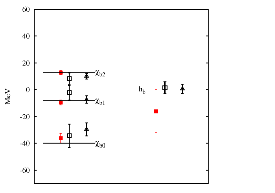
Figure 16: $P$-wave spin splittings. Closed and open symbols are from coarse and fine lattices respectively. Squares and triangles denote unquenched and quenched results respectively. The unquenched results are from the ensembles in Table 1 that include the lightest light quark mass in the quark vacuum polarization at the coarse and fine lattice spacing values. Errors are statistical/fitting only but include errors from determining the lattice spacing as in Figure 14. There is an additional 25% systematic error as discussed in the text. Lines give the experimental results where available pdg .

VII.2 $P$-wave fine structure

Both ground and radially excited ${}^{3}P_{0,1,2}$ states ($\chi_{bJ}$ and $\chi_{bJ}^{\prime}$ are well measured in the $\Upsilon$ system. No ${}^{1}P_{1}$ ($h_{b}^{(\prime)}$) states have been seen. We are able to predict that the ground state $h_{b}$ should lie within 6 MeV of the spin-average of the $\chi_{b}$ states i.e. at 9900(3)(6) MeV, where 3 is the experimental error pdg . We describe our analysis in more detail below, including a discussion of how well our ${}^{3}P$ results match experiment.

The $P$-wave fine structure was only calculated for a limited selection of ensembles. For the majority of runs, we were unable to resolve excited splittings well and consequently show only the ground state results. The errors given are those from bootstrapping the fits of the individual correlators on the coarse and fine ensembles. For the super-coarse ensembles they come directly from the fits. Tables 19, 20, 21 give the energy splittings in lattice units. The lattice representation for the ${}^{3}P_{2}$ states used was the $E$ representation on the coarse and fine lattices. Any difference between the energy in the $E$ representation and in the $T$ representation is a lattice artefact. We give both for the super-coarse ensemble where such artefacts will be largest, but even there we cannot resolve any difference. The Tables also give the dimensionless ratio:

$$\frac{M(1^{3}P_{1})-M(1^{3}P_{0})}{M(1^{3}P_{2})-M(1^{3}P_{1})}.$$ (20)

The results obtained for this ratio have sizeable errors but are consistent on both unquenched and quenched ensembles with the experimental value of 1.65(9) pdg .

Figure 16 plots the lattice results for the ground state $P$-wave splittings, each relative to the spin average. We use the $2S-1S$ lattice spacing values to convert to physical units. The plot shows the coarse and fine unquenched and fine quenched results only since the results on the super-coarse ensemble have error bars which are too large to be useful, although they are consistent with the others. The Figure shows that the size of the quenched $P$-wave splittings are smaller than experiment. The results on the coarse 2+1 flavor configurations look consistent with experiment, as do the fine 2+1 flavor results, although their errors are rather large. The errors shown on the plot are from statistics/fitting only and from determining the lattice spacing. We double the lattice spacing error as for the hyperfine splitting but in general this is negligible compared to the statistical/fitting error of the $P$-wave splittings themselves. We now discuss the sources of systematic error.

As for the hyperfine splitting, the largest sources of systematic error potentially are the unknown radiative corrections to relevant spin-dependent terms in the NRQCD action. Two terms are relevant for $P$-wave fine structure which complicates the picture - the $\sigma\cdot B$ term and the $\sigma\cdot(D\times E)$ term - with coefficients $c_{4}$ and $c_{3}$ respectively. There are combinations of $P$-wave splittings, however, that can be compared to experiment to give non-perturbative information to fix these coefficients.

The $\sigma\cdot(D\times E)$ term gives rise to a coupling between spin and orbital angular momentum and a term in the mass of each state which depends on the expectation value of $L\cdot S$ multiplied by $c_{3}$. The $\sigma\cdot B$ term gives rise to a mass term proportional to $c_{4}^{2}$ and either $S\cdot S$, which is the same for all ${}^{3}P$ states, or the combination $3(S\cdot\hat{n}S\cdot\hat{n})-S^{2}$ which does distinguish between ${}^{3}P$ states. From the expectation values of these operators in the different $\chi_{b}$ states cdschladming we see that the combination

$$5M(\chi_{b2})-3M(\chi_{b1})-2M(\chi_{b0})$$ (21)

is proportional to $c_{3}$ and independent of $c_{4}$. The experimental result for this combination is 165(4) MeV and our lattice result on the coarse unquenched ensemble is 164(16) MeV. This indicates that $c_{3}$ is 1.0 to within an error of 10%. The combination

$$M(\chi_{b2})-3M(\chi_{b1})+2M(\chi_{b0})$$ (22)

is proportional to $c_{4}^{2}$ and independent of $c_{3}$. The experimental result for this combination is -46(3) MeV and our lattice result is -31(7) MeV. The lattice result is 30% low but with a large error, so that the difference is 2$\sigma$. The limits on $c_{4}^{2}$ from the $B_{s}$ hyperfine splitting, i.e. 1.0 with an error of 20%, are to be preferred for accuracy.

We conclude from this that the systematic error from radiative corrections to the leading spin-dependent terms is $\cal{O}$(20%) in the ${}^{3}P$ fine structure. We also expect a 10% error from higher order relativistic corrections. Discretisation errors are not expected to be as severe here as for the hyperfine splitting because the $P$-wave states have a larger radial extent than the $S$-wave and, in potential model language, the potentials that give rise to the relevant splittings are not so concentrated at the origin. Allowing for as much as a 10% error from discretisation effects, however, the total expected systematic error in the ${}^{3}P$ fine structure in this calculation is 25%. Future calculations will include radiative and relativistic corrections and will then resolve the ${}^{3}P$ fine structure much more accurately.

Figure 16 also shows the splitting between the spin-average of the ${}^{3}P$ states and the ${}^{1}P_{1}$. This splitting is a result of the same $S\cdot S$ coupling that produces the hyperfine splitting but it is expected to vanish for $P$-wave states in a potential model because the interaction is focussed at the origin. We have no signal for such a splitting with an error of 5 MeV on the fine unquenched ensemble from statistics/fitting and the determination of the lattice spacing. Systematic errors arise from radiative corrections to $c_{4}^{2}$, which we take to be 20% as above, and relativistic and discretisation errors which we take to be 10% each. This gives a splitting of zero with an error of 6 MeV.

$0.01/0.05$ $1^{3}D_{3}-1^{3}D_{2}$ 0.010(15) $1^{3}D_{2}-1^{1}D_{2}$ 0.002(18)

Table 22: $D$-wave fine structure for the 2+1 flavor 0.01/0.05 coarse ensemble. Energies are given in lattice units. Errors are statistical/fitting only and obtained directly from the fits.

VII.3 $D$-wave fine structure

The fine structure in the $D$-wave sector is on a smaller scale than for $S$-wave and $P$-wave, as expected. We are unable to resolve any splittings there with errors of around 10 MeV. $D$-wave fine structure was only studied on the 2+1 flavor 0.01/0.05 coarse ensemble. We looked at the ${}^{1}D_{2}$ state (using the $T$ representation), the ${}^{3}D_{2}$ (using the $E$ representation) and the ${}^{3}D_{3}$ (using the $A$ representation) upspaper . Table 22 gives splittings in lattice units with errors obtained directly from the fits.

VIII The $\Upsilon$ leptonic width

The width of $\Upsilon$ decay to two leptons, $\Gamma_{ee}$, can be well measured experimentally pdg ; cleolw . The matrix element that gives rise to the decay can also be calculated on the lattice and we describe that calculation here. Our most accurate result is for the ratio between the $\Upsilon^{\prime}$ and $\Upsilon$ of $\Gamma_{ee}M_{\Upsilon(nS)}^{2}$. We obtain 0.48(5) compared to the recent preliminary experimental result of 0.517(10) cleolw . Below we describe the calculation in more detail and the sources of error, along with improvements that will shortly be possible in the result.

On the lattice $\Gamma_{ee}$ is calculated from the matrix element of the $b\overline{b}$ vector current between the $\Upsilon$ and the vacuum. The decay width is then given by perkins :

$$\Gamma_{ee}(nS)=16\pi\alpha_{em}^{2}e_{b}^{2}\frac{\langle\Upsilon_{n}|J_{v}|0\rangle^{2}}{6M^{2}_{\Upsilon(nS)}}({Z_{match}})^{2}$$ (23)

where $\alpha_{em}$ is the electromagnetic coupling constant, $e_{b}$ is the charge on a $b$ quark in units of the charge on an electron and $M_{\Upsilon(nS)}$ is the mass of the $n$th radial excitation of the $\Upsilon$. This formula assumes a non-relativistic normalisation of states, $\langle\Upsilon|\Upsilon\rangle$ = 1. $Z_{match}$ is the renormalisation constant, $1+z^{(1)}\alpha_{s}+\ldots$, required to match the lattice vector current to a continuum renormalisation scheme. The lattice vector current constructed out of NRQCD fields has leading term $\chi^{{\dagger}}_{b}{\bf{\sigma}}\psi_{b}$ where $\psi$ annihilates a $b$ quark and $\chi^{{\dagger}}$ an anti-$b$. There are sub-leading terms which take account of relativistic and discretisation corrections required to match the continuum current to higher order. This matching can be done perturbatively and is in progress horgan . The calculation is entirely analogous to that for the $B$ meson decay constant, whose $Z_{match}$ has been calculated through 1-loop junkocolin , including the effect of higher order current corrections.

$0.0082/0.082$ $a^{3/2}\Psi_{1}(0)$ 0.5184(10) $a^{3/2}\Psi_{2}(0)$ 0.499(20)

Table 23: Results for the leading order piece of the lattice heavy-heavy vector current matrix element between the $\Upsilon$ and the vacuum, also known as the ‘wavefunction at the origin’. Results are given in lattice units for the $\Upsilon$ ($\Psi_{1}(0)$) and for the $\Upsilon^{\prime}$ ($\Psi_{2}(0)$) for the super-coarse ensembles. Errors are statistical/fitting only.

$0.01/0.05$ $0.02/0.05$ $0.03/0.05$ $0.05/0.05$ 0.02 Quenched $a^{3/2}\Psi_{1}(0)$ 0.30149(66) 0.29830(59) 0.29441(67) 0.29142(78) 0.28563(53) 0.26152(50) $a^{3/2}\Psi_{2}(0)$ 0.2446(66) 0.2401(50) 0.224(14) 0.237(11) 0.230(11) 0.2346(48)

Table 24: Results for the leading order piece of the lattice heavy-heavy vector current matrix element between the $\Upsilon$ and the vacuum, also known as the ‘wavefunction at the origin’. Results are given in lattice units for the $\Upsilon$ ($\Psi_{1}(0)$) and for the $\Upsilon^{\prime}$ ($\Psi_{2}(0)$) for the coarse ensembles. Errors are statistical/fitting only.

$0.0062/0.031$ $0.0124/0.031$ Quenched $a^{3/2}\Psi_{1}(0)$ 0.17666(49) 0.17796(44) 0.15159(31) $a^{3/2}\Psi_{2}(0)$ 0.1357(24) 0.1372(19) 0.1298(17)

Table 25: Results for the leading order piece of the lattice heavy-heavy vector current matrix element between the $\Upsilon$ and the vacuum, also known as the ‘wavefunction at the origin’. Results are given in lattice units for the $\Upsilon$ ($\Psi_{1}(0)$) and for the $\Upsilon^{\prime}$ ($\Psi_{2}(0)$) for the fine ensembles. Errors are statistical/fitting only.

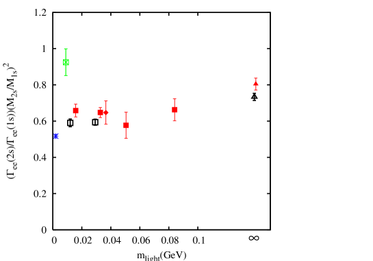
Figure 17: The ratio of leptonic width times mass squared for the 1st excited state of the $\Upsilon$ to that of the ground state. Crossed squares are from super-coarse unquenched ensembles, closed squares from coarse unquenched ensembles and open squares from the fine unquenched ensembles. The closed and open triangles are from the coarse and fine quenched ensembles respectively. The closed diamond is from the coarse $n_{f}=2$ ensemble. The burst represents the current experimental result.

For the leading order current only it is easy to extract the matrix element from our existing results with no further work. It is simply the amplitude in the $n$th $\Upsilon$ state of the local (delta) smearing, i.e. $a(loc,n)$ from equation 6, appropriately normalised. In potential model language this is known as the wavefunction at the origin, $\Psi(0)$, and is obtained from the lattice results when the correlators are divided by the product of the number of colors (3) and the number of non-relativistic spins (2). Then $\Psi(0)=\langle\Upsilon_{n}|J_{v}|0\rangle/\sqrt{6}$, accounting for the factor of 6 in the denominator of Equation 23. Results for this quantity are given in lattice units in tables 23, 24 and  25 for the super-coarse, coarse and fine ensembles respectively.

There will be an $\cal{O}$$(\alpha_{s})$ systematic error from $Z_{match}$ if we try to calculate $\Gamma_{e+e-}$ directly from these numbers. Instead we form the ratio:

$$\frac{\Gamma_{ee}(2S)M^{2}_{\Upsilon(2S)}}{\Gamma_{ee}(1S)M^{2}_{\Upsilon(1S)}}=\frac{|\Psi_{2}(0)|^{2}}{|\Psi_{1}(0)|^{2}}$$ (24)

in which the $Z_{match}$ factor for the current cancels. We then expect to be able to determine this ratio from the leading current with errors coming from the matrix elements of relativistic corrections to the current.

Figure 17 shows this ratio for our lattice results on super-coarse, coarse and fine ensembles. The current experimental result pdg is given by the burst. The lattice results in the quenched approximation are in strong disagreement with experiment. Previous quenched results also indicated this, but less precisely upspaper ; scaling . The results move down towards experiment once light quark vacuum polarization effects are included and the light quark mass falls. However, the results on the unquenched ensembles with lightest light quark mass are still some way from experiment. The plot shows no dependence on light quark mass for the most chiral ensembles, as expected. We therefore do not attempt a chiral extrapolation but now look at lattice spacing dependence for those results with lightest light quark mass.

The quenched results for the ratio and those from the most chiral unquenched ensembles are plotted against the square of the lattice spacing in Figure 18. This plot shows a significant dependence on $a^{2}$, indicating discretisation errors in the results. These may come from the current operator or from the action at the level of $\alpha_{s}a^{2}$ and it is not clear which is the most important at this stage. The wavefunction at the origin is a very short-distance quantity (akin to the hyperfine splitting) and it is reasonable for it to show significant discretisation effects when other quantities, such as radial and orbital splittings in the spectrum, do not.

We can directly calculate the leptonic width for the $\Upsilon$ and $\Upsilon^{\prime}$ in the absence of $Z_{match}$ to see how each behaves. We use the formula given in Equation 23 taking $\alpha_{em}(m_{b})$ = 1/132 erler . We obtain a value $\Gamma_{ee}$=1.43(7) keV for the $\Upsilon$ from the super-coarse 2+1 flavor unquenched ensemble, 1.32(1) keV from the coarse 2+1 flavor 0.01/0.05 unquenched configurations and 1.28(1) keV from the fine 2+1 flavor 0.0062/0.031 configurations. The error given here comes only from the error in the determination of the ($2S-1S$) lattice spacing which appears cubed in this result. The fine lattice numbers is slightly lower than the recent preliminary experimental result, 1.34(2) keV cleolw . The absence of $Z_{match}$ or higher order corrections gives a sizeable additional systematic error to the lattice result, but there is at least nothing to indicate that large systematic shifts are required to match experiment. The quenched results for the $\Upsilon$ are significantly lower at 1.0 keV on the fine lattices. For the $\Upsilon^{\prime}$ there is more sign of discretisation in the bare leading-order matrix element. From this, we obtain $\Gamma_{e+e-}$ = 1.2(1) keV on the super-coarse unquenched ensemble, 0.77(5) keV on the coarse unquenched lattices and 0.67(3) keV on the fine unquenched lattices, with errors as above. This is not inconsistent with the fact that the excited state has more structure in its ‘wavefunction’ and therefore might be more susceptible to short distance errors than the ground state. The fine lattice result is slightly higher than the recent preliminary experimental value of 0.616(13) keV cleolw .

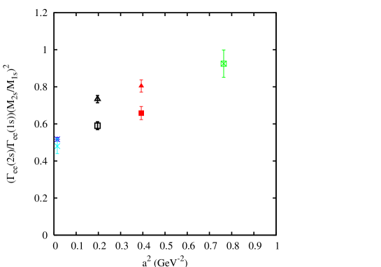
Figure 18: The dependence on $a^{2}$ of the ratio of leptonic width times mass squared for the 1st excited state of the $\Upsilon$ to that of the ground state. Crossed, closed and open squares are from the most chiral of the super-coarse, coarse and fine unquenched lattices respectively and closed and open triangles are from quenched lattices. The burst represents the current experimental result, and the cross below this is our continuum extrapolated result, including an estimate of the leading relativistic corrections as described in the text.

As for the hyperfine splitting earlier (Equation 19) we consider $a$-dependence in the ratio of Equation 24 of the form

$${\rm ratio}(a)={\rm ratio}(0)(1+(\Lambda a)^{2}+\ldots).$$ (25)

However, here the $a$-dependence is stronger than for the hyperfine splitting ($\Lambda\approx$ 900 MeV) and the super-coarse results are therefore correspondingly less reliable. Using again a constrained fit we find a continuum value for the ratio of 0.50(4) for the leading order current. The 8% error is a combination of the statistical/fitting error and the effect of discretisation errors.

The higher order relativistic current corrections are given by operators of the form joneswol :

$$\chi^{{\dagger}}(\frac{1}{8(M_{b}^{0})^{2}}(\Delta^{(2){\dagger}}\sigma+\sigma\Delta^{(2)}-2(\mbox{\boldmath$\sigma$}\cdot{\bf{\bf\Delta}}^{{\dagger}})\sigma(\mbox{\boldmath$\sigma$}\cdot{\bf{\bf\Delta}}))\psi.$$ (26)

For an $\Upsilon$ at zero momentum the $\Delta^{(2)}$ operator acting on either quark or anti-quark will give the same matrix element. This is similarly true for the operator made from one derivative on each. The $i$th component of the correction operator then becomes:

$$\chi^{{\dagger}}\frac{1}{4(M_{b}^{0})^{2}}(\frac{2}{3}\Delta^{(2){\dagger}}\sigma_{i}+2D_{ij}\sigma_{j})\psi.$$ (27)

where $D_{ij}={\bf\Delta}_{i}{\bf\Delta}_{j}-\Delta^{(2)}/3$. The second term above is the piece which couples to a $D$-wave state upspaper and gives a leptonic width to the ${}^{3}D_{1}$ state. The first term is the one that we are concerned with and that gives a relativistic correction to the $S$-wave leptonic width of the form $\chi^{{\dagger}}\Delta^{(2)}\sigma/6(M_{b}^{0})^{2}\psi$. We calculate the matrix element of this term by inserting a $\Delta^{(2)}$ operator at the correlator sink. We then fit the correlator with the insertion simultaneously with the other correlators used to get the matrix element of the leading order current above. We have done this for the 0.01/0.05 2+1 flavor coarse ensemble only. There the current correction matrix element (in lattice units) is -0.0107(2) for the $\Upsilon$ and -0.0131(4) for the $\Upsilon^{\prime}$, i.e. a 3.5% and 5.4% correction to the leading matrix element respectively. This induces a further 4% reduction in the ratio of leptonic width times mass squared for the 2$S$ to 1$S$. The size of the relativistic corrections and the overall shift from their difference is perfectly in keeping with expectations based on power-counting in $v^{2}$. Higher order relativistic corrections are then likely to be negligible.

We apply this shift of 4% to our continuum leading order current result. We also add an additional 4% error ($\alpha_{s}v^{2}$) to allow for missing radiative corrections to the relativistic corrections in the ratio (radiative corrections to the leading order term cancel, as discussed earlier). This gives our final answer for the ratio of Equation 24 of 0.48(5), to be compared to the recent preliminary experimental result cleolw of 0.517(10). Both of these are also marked on Figure 18. Our result is compatible with experiment but not as precise. Our 10% error is dominated by the fact that the lattice results depend strongly on the lattice spacing.

The lattice calculation of $\Gamma_{ee}$ can be significantly improved. Once the renormalisation of the leading and sub-leading lattice NRQCD current operators is calculated, we will be able to compute the $\Gamma_{ee}$ results for each radial excitation of the $\Upsilon$ separately with systematic errors at the 10% level coming from unknown $\alpha_{s}^{2}$ terms in $Z_{match}$ horgan . We will also discover whether the current corrections contain a sizeable contribution in the form of a discretisation correction, so that the scaling with lattice spacing improves. As discussed earlier, the ratio of leptonic width times mass squared will be more precise than this because the errors will be set by $v^{4}$ corrections to the current and $\alpha_{s}^{2}$ errors in the $v^{2}$ current correction piece. These errors should be at the level of a few percent.

IX Conclusion

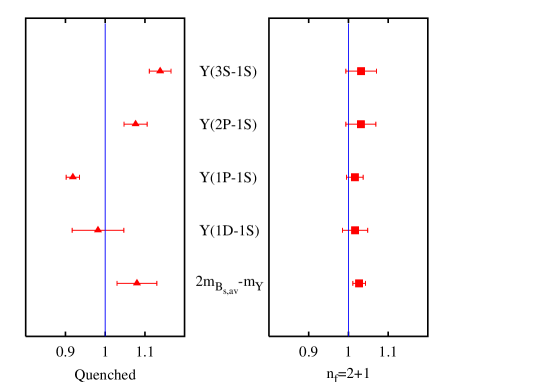
Figure 19: The ratio of lattice results to experiment for various mass splittings involving $b$ quarks. The results are for quenched simulations (left) and simulations incorporating $2+1$ flavors of sea quarks (right). All the unquenched results come from this work. We have taken results from the most chiral coarse lattice ensemble since those have the best errors in general. Errors include statistical/fitting errors for the quantity in question and those from determining the lattice spacing. The top three quenched results come from this work, but the lower two are estimates from earlier work. The quenched $1D-1S$ splitting is taken from campbelm using the ${}^{1}D_{2}$ state. The quenched $2m_{B_{s}}-m_{\Upsilon}$ splitting is estimated from joachim , adjusted to use the lattice spacing from the $\Upsilon$ $2S-1S$ spacing.

We have presented a state-of-the-art calculation for $\Upsilon$ spectroscopy in lattice QCD. The major improvement over previous calculations is that we now have results on gluon field configurations that include 2+1 flavors of sea quarks with the $u/d$ quark masses within reach of their physical values. This means, as we demonstrate here, that it is now possible to fix the parameters of the QCD Lagrangian unambiguously. The $\Upsilon$ system is a good place to test this because of the large number of well-determined excited states. Figure 19 shows a ‘ratio’ plot of lattice results from this paper compared to experiment. The unquenched results on the right are in striking agreement with experiment compared to the quenched results on the left. This ratio plot differs slightly from that in us for the quenched results because of improved fits for the quenched ensembles here.

Our results enable us to determine physical values for the parameters $r_{0}$ (0.469(7) fm) and $r_{1}$ (0.321(5) fm), often used to compare lattice spacing values between different ensembles in lattice calculations.

Further improvements to the calculation of radial and orbital excitation energies will require further improvements to the NRQCD action, in particular the calculation of radiative corrections to $v^{4}$ and $a^{2}$ terms. This is in progress. Statistical precision can also be improved since double the number of configurations used here are available as well as further configurations with lighter sea quark masses milc1 ; milc2 . Precision on $P$ and $D$-wave states would be improved by better smearing.

Our result for the $b$ quark mass in the $\overline{MS}$ scheme at its own scale is 4.4(3) GeV, using a 1-loop matching of the lattice to the continuum. A 2-loop calculation of the heavy quark self-energy would reduce the error significantly on the $b$ quark mass as well as make the remaining error estimate more reliable by fixing the scale for $\alpha_{s}$ in the matching coefficient. This is currently underway.

The fine structure in the spectrum is only calculated to leading order here, so sizeable systematic errors remain. We are able nevertheless to predict the ground-state hyperfine splitting more accurately than in the past and the radially excited hyperfine splitting for the first time. Our results are 61(14) MeV and 30(19) MeV respectively. To reduce the errors requires, as above, the determination of radiative corrections to the leading spin-dependent terms in the NRQCD action and the inclusion of sub-leading terms. Further improvement to reduce discretisation errors is also an issue.

The calculation of the leptonic width for $\Upsilon$ and $\Upsilon^{\prime}$ is an important example of a simple decay rate that can be calculated in lattice QCD, without the ambiguity that arises from potential models eq . Our results on unquenched configurations for the ratio of leptonic widths (multiplied by squared masses) for $\Upsilon^{\prime}$ and $\Upsilon$ show a much closer agreement with experiment than those on quenched configurations. Sizeable discretisation errors prevent us giving a very accurate result here, but we obtain 0.48(5) for the ratio. Further precision will come from the calculation of the renormalisation constant required to match the lattice and continuum currents responsible for the decay. The calculation will yield an improved current operator with reduced discretisation errors. This is also underway.

Acknowledgements We thank members of the MILC collaboration for making their configurations available, and R. Sugar, D. Toussaint and S. Gottlieb for help with reading them. We thank R. Horgan, Q. Mason, M. Nobes, J. Pivarski and H. Trottier for useful discussions. The computing was done on the UKQCD alpha cluster at the University of Glasgow funded by PPARC and on the Fermilab cluster and at NERSC funded by the U.S. Department of Energy. We are grateful to PPARC, the DoE and the NSF for support.

References

- (1) Fermilab, HPQCD, MILC, UKQCD collaborations, C. T. H. Davies et al, Phys. Rev. Lett. 92, 022001 (2004), hep-lat/0304004.
- (2) HPQCD, MILC, UKQCD collaborations, C. Aubin et al, Phys. Rev. D70, 031504 (2004), hep-lat/0405022.
- (3) MILC collaboration, C. Aubin et al, hep-lat/0407028.
- (4) Fermilab, HPQCD collaborations, I. Allison, C. T. H. Davies, A. Gray, A.S. Kronfeld, P. B. Mackenzie, J. N. Simone, Phys. Rev. Lett. 94, 172001 (2005), hep-lat/0411027.
- (5) Fermilab, MILC collaborations, C. Aubin et al, hep-ph/0408306.
- (6) C. W. Bernard et al, Phys. Rev. D64, 054506 (2001), hep-lat/0104002.
- (7) C. Aubin et al, Phys. Rev. D70, 094505 (2004), hep-lat/0402030.
- (8) MILC collaboration, private communication.
- (9) The action was first given in: G. P. Lepage, Phys. Rev. D59, 074502 (1999), hep-lat/9809157. See the following for studies of its performance: K. Orginos, D. Toussaint, R. L. Sugar, Phys. Rev. D60, 054503 (1999), hep-lat/9903032; MILC collaboration, C. Bernard et al, Phys. Rev. D61, 111502 (2000), hep-lat/9912018.
- (10) M. Alford, W. Dimm, G. P. Lepage, G. Hockney and P. B. Mackenzie, Phys. Lett. B361 (1995) 87, hep-lat/9507010.
- (11) M.Nobes, hep-lat/0501009.
- (12) B. A. Thacker and G. P. Lepage, Phys. Rev. D43 (1991) 196.
- (13) G. P. Lepage et al, Phys. Rev. D46, 4052 (1992), hep-lat/9205007.
- (14) C. T. H. Davies, K. Hornbostel, A. Langnau, G. P. Lepage, A. Lidsey, J. Shigemitsu, J. Sloan, Phys. Rev. D50, 6963 (1994), hep-lat/9406017.
- (15) C. Morningstar, Phys. Rev. D50 (1994) 5902, hep-lat/9406002.
- (16) G. P. Lepage and P. Mackenzie, Phys. Rev. D48 (1993) 2250.
- (17) The value of does affect the value of the ground state energy as is clear from comparing Tables 5 and 7. The dependence on can be seen in perturbation theory or in a mean field approach nakhleh which gives a reasonably good quantitative description of the results.
- (18) M. Nobes, private communication.
- (19) C. T. H. Davies, K. Hornbostel, G. P. Lepage, A. Lidsey, J. Shigemitsu and J. H. Sloan, Phys. Lett. B345 (1995) 42, hep-ph/9408328.
- (20) C. T. H. Davies, K. Hornbostel, G. P. Lepage, A. Lidsey, P. McCallum, J. Shigemitsu, J. H. Sloan, Phys. Rev. D58, 054505 (1998), hep-lat/9802024.
- (21) S. Groote and J. Shigemitsu, Phys. Rev. D62, 014508 (2000), hep-lat/0001021.
- (22) G. P. Lepage et al, Nucl. Phys. B (Proc. Suppl. 106) (2002)12, hep-lat/0110175.
- (23) S. Eidelman et al, Phys. Lett. B592 (2004) 1.
- (24) C. T. H. Davies, K. Hornbostel, G. P. Lepage, P.McCallum, J. Shigemitsu, J. H. Sloan, Phys. Rev. D56 (1997) 2755.
- (25) N. Eicker et al, Phys. Rev. D57, 4080 (1998), hep-lat/9709002.
- (26) CP-PACS collaboration, T. Manke et al, Phys. Rev D62, 114508 (2000), hep-lat/0005022.
- (27) UKQCD collaboration, L. Marcantonio, P. Boyle, C. T. H. Davies, J. Hein, J. Shigemitsu, Nucl. Phys. B (Proc. Suppl.94), 363 (2001), hep-lat/0011053.
- (28) R. Sommer, Nucl. Phys. B411 (1994) 839, hep-lat/9310022.
- (29) CLEO collaboration, G. Bonvicini et al, Phys. Rev. D70:32001 (2004), hep-ex/0404021.
- (30) M. Alford, T. R. Klassen and G. P. Lepage, Nucl. Phys. B496 (1997) 377, hep-lat/9611010.
- (31) Y. Kayaba et al, Nucl. Phys. B (Proc. Suppl.) 140 (2005) 479, hep-lat/0409086.
- (32) J. Shigemitsu et al, Proceedings of LAT04, Nucl. Phys. B(Proc. Suppl. 140) (2005) 464, hep-lat/0408019.
- (33) C. T. H. Davies, K. Hornbostel, A. Langnau, G. P. Lepage, A. Lidsey, C. J. Morningstar, J. Shigemitsu, J. Sloan, Phys. Rev. Lett. 73 (1994) 2654, hep-lat/9404012.
- (34) E. Gulez, J. Shigemitsu and M. Wingate, Phys. Rev. D69:074501 (2004), hep-lat/0312017.
- (35) Q. Mason et al, Phys. Rev. Lett. (in press), hep-lat/0503005; Q. Mason and H. Trottier, in preparation.
- (36) S. J. Brodsky, G. P. Lepage and P. B. Mackenzie, Phys. Rev. D28 (1983) 228.
- (37) C, Morningstar, private communication from the calculation of colin2 , using a slightly different NRQCD action and an unimproved gluon action.
- (38) NRQCD collaboration, K. Hornbostel, Nucl. Phys. B (Proc. Suppl. 73) (1999) 339, hep-lat/9809177.
- (39) K. Melnikov and T. van Ritbergen, Phys. Lett. B482 (2000) 99, hep-ph/9912391.
- (40) A. Ali Khan et al, Phys. Rev. D62:054505 (2000), hep-lat/9912034.
- (41) Belle collaboration, S.-K. Choi et al, Phys. Rev. Lett. 89:102001 (2002).
- (42) HPQCD collaboration, in preparation.
- (43) H. Trottier, Phys. Rev. D55 (1997) 6844, hep-lat/9611026; T. Manke et al, Phys. Lett. B468 (1997) 308, hep-lat/9706003; N. H. Shakespeare and H. D. Trottier, Phys. Rev. D58:034502 (1998), hep-lat/9802038.
- (44) C. Davies, Springer Lecture notes in Physics, Eds Gausterer, Lang, 1998, hep-ph/9710394.
- (45) Jean Duboscq, CLEO, talk at the HEP2005 Europhysics conference, Lisbon, July 2005, www.lip.pt/events/2005/hep2005/talks/session5.html.
- (46) See, for example, D. H. Perkins, Introduction to High Energy Physics, 3rd Ed. (Addison-Wesley, Reading, MA).
- (47) G. von Hippel, PhD thesis, University of Cambridge, 2003; R. Horgan, private communication.
- (48) C. J. Morningstar and J. Shigemitsu, Phys. Rev. D57 (1998) 6741, hep-lat/9712016.
- (49) J. Erler, Phys. Rev. D59:054008 (1999), hep-ph/9803453.
- (50) B. D. Jones and R. M. Woloshyn, Phys. Rev. D60:014502(1999), hep-lat/9812008.
- (51) E. Eichten and C. Quigg, Phys. Rev. D52 (1995) 1726, hep-ph/9503356.
- (52) M. Campbell, MSc thesis, University of Glasgow, 1998. We use the average of the and (since these seem more reliable than the corresponding results) and combine it with the energy and value from upspaper .
- (53) J. Hein et al, Phys. Rev. D62:074503 (2000), hep-ph/0003130. We take results for unimproved glue at =6.2 and combine with results from scaling , after adjustment to use the lattice spacing from the splitting consistently, including for the quark mass. This can only be done to a limited extent because the original calculations used a different lattice spacing, in an attempt to reduce errors from quenching. This result should then be taken as indicative only.