DESY 05-113 SFB/CPP-05-29 July 2005
Quenched Scaling of Wilson twisted mass fermions

We investigate the scaling behaviour of quenched Wilson twisted mass fermions at maximal twist applying two definitions of the critical mass. The first definition uses the vanishing of the pseudoscalar meson mass $m_{\rm PS}$ while the second employs the vanishing of the PCAC quark mass $m_{\rm PCAC}$. We confirm in both cases the expected $O(a)$ improvement. In addition, we show that the PCAC quark mass definition leads to substantially reduced $O(a^{2})$ cut-off effects even when the pseudoscalar meson mass $m_{\rm PS}$ is as small as $270$ MeV. At a fixed value of $m_{\rm PS}$ we perform continuum limits for the vector meson mass $m_{V}$ and for the pseudoscalar decay constant $f_{\rm PS}$ and discuss the renormalisation constant $Z_{V}$ of the vector current.

1 Introduction

Knowing the scaling behaviour of a given lattice action is an important step towards performing a controlled continuum limit of physical observables. The important result that Wilson fermions with a twisted mass term added [1] lead, at full twist, to an automatic $O(a)$-improvement of correlators [2] without the need of additional improvement terms makes it particularly interesting to test this formulation of lattice QCD with numerical simulations. In this paper we will use lattice spacings ranging from $a=0.05$ fm to $a=0.17$ fm and pseudoscalar meson masses from $m_{\rm PS}=1180$ MeV down to $m_{\rm PS}=270$ MeV in order to perform a detailed scaling test of Wilson twisted mass fermions. In this way, we extend a first scaling test [3] substantially. All our simulations presented here are done in the quenched approximation, see also [4, 5, 6, 7] for further quenched results of Wilson twisted mass QCD. Let us mention that also full QCD simulations with this approach have already been performed and proved to be very useful in studying the phase structure of lattice QCD with Wilson fermions [8, 9, 10, 11, 12].

A basic ingredient to have automatic $O(a)$-improvement is the tuning of the bare quark mass to its critical value. In the language of twisted mass QCD (tmQCD) this procedure corresponds to fix the twist angle to $\pi/2$. In the present work, we will employ two definitions for the critical mass. The first is the point where the pseudoscalar meson mass vanishes, the second, where the PCAC quark mass vanishes. In the following we will refer to the first situation as the “pion definition” and to the second situation as the “PCAC definition” of the critical point. Both definitions should lead to $O(a)$-improvement, but they can induce very different $O(a^{2})$ effects, in particular at small pseudoscalar meson masses. Indeed, in ref. [4, 13] we reported that the pion definition can have substantial $O(a^{2})$ effects which are amplified when the quark mass becomes small and violates the inequality $\mu>a\Lambda^{2}$ (where $\mu$ is the bare quark mass, i.e. the parameter which provides at full twist a mass to the pseudoscalar meson). On the other hand, when the PCAC definition of the critical mass is used, these particular kind of $O(a^{2})$ cut-off effects are dramatically reduced as was demonstrated in [5, 7]. The effect of reducing $O(a^{2})$ artefacts has been theoretically studied in chiral perturbation theory in refs. [14, 15] and put on a more general basis in ref. [16].

In this paper, we employ the pion and the PCAC definitions of the critical mass to study the scaling behaviour of the pseudoscalar meson decay constant and the vector meson mass. The renormalisation constant $Z_{V}$ of the vector current is also presented for three values of the lattice spacing.

2 Wilson twisted mass fermions

Wilson twisted mass fermions can be arranged to be $O(a)$ improved without employing specific improvement terms [2]. The Wilson tmQCD action in the twisted basis can be written as

$$S[U,\psi,\bar{\psi}]=a^{4}\sum_{x}\bar{\psi}(x)(D_{W}+m_{0}+i\mu\gamma_{5}\tau_{3})\psi(x)\;,$$ (1)

where the Wilson-Dirac operator $D_{\rm W}$ is given by

$$D_{\rm W}=\sum_{\mu=0}^{3}\frac{1}{2}[\gamma_{\mu}(\nabla_{\mu}^{*}+\nabla_{\mu})-a\nabla_{\mu}^{*}\nabla_{\mu}]$$ (2)

and $\nabla_{\mu}$ and $\nabla_{\mu}^{*}$ denote the usual forward and backward derivatives. We refer to [4] for further unexplained notations. The definition of the critical mass $m_{c}$ will be discussed in detail in the next section.

We extract pseudoscalar and vector meson masses from the correlation functions at full twist ($m_{0}=m_{c}$):

$$C_{P}^{a}(x_{0}) = a^{3}\sum_{\mathbf{x}}\langle P^{a}(x)P^{a}(0)\rangle\quad a=1,2$$ (3)

$$C_{A}^{a}(x_{0}) = \frac{a^{3}}{3}\sum_{k=1}^{3}\sum_{\mathbf{x}}\langle A_{k}^{a}(x)A_{k}^{a}(0)\rangle\quad a=1,2$$ (4)

$$C_{T}^{a}(x_{0}) = \frac{a^{3}}{3}\sum_{k=1}^{3}\sum_{\mathbf{x}}\langle T_{k}^{a}(x)T_{k}^{a}(0)\rangle\quad a=1,2$$ (5)

where we consider the usual local bilinears $P^{a}=\bar{\psi}\gamma_{5}\frac{\tau^{a}}{2}\psi$, $A_{k}^{a}=\bar{\psi}\gamma_{k}\gamma_{5}\frac{\tau^{a}}{2}\psi$ and $T_{k}^{a}=\bar{\psi}\sigma_{0k}\frac{\tau^{a}}{2}\psi$.

The untwisted PCAC quark mass $m_{\textrm{PCAC}}$ can be extracted from the ratio

$$m_{\textrm{PCAC}}=\frac{\sum_{\mathbf{x}}\langle\partial_{0}A_{0}^{a}(x)\;P^{a}(0)\rangle}{2\sum_{\mathbf{x}}\langle P^{a}(x)P^{a}(0)\rangle}\quad a=1,2\;.$$ (6)

Using the exact lattice PCVC relation

$$\langle\partial^{*}_{\mu}\tilde{V}^{a}_{\mu}(x)O(0)\rangle=-2\mu\epsilon^{3ab}\langle P^{b}(x)O(0)\rangle\qquad a=1,2$$ (7)

(where $\partial^{*}_{\mu}$ is the lattice backward derivative, $\tilde{V}^{a}_{\mu}$ is the point-splitted vector current and $O$ is a local lattice operator) we can also compute the pseudoscalar meson decay constant at maximal twist without requiring any renormalisation constant (see [17, 18, 3]):

$$f_{\rm PS}=\frac{2\mu}{m_{\rm PS}^{2}}|\langle 0|P^{a}|{PS}\rangle|\qquad a=1,2\;,$$ (8)

where $m_{\rm PS}$ is the charged pseudoscalar mass and $|{PS}\rangle$ denotes the corresponding pseudoscalar state.

If one now is interested in using the local definition of the vector current $V^{a}_{\mu}=\bar{\psi}\gamma_{\mu}\frac{\tau^{a}}{2}\psi$, $\tilde{V}^{a}_{\mu}$ has to be substituted with $Z_{V}V^{a}_{\mu}$ in eq. (7) and the relation is now valid only up to order $O(a^{2})$ lattice artifacts. This relation allows for a determination of $Z_{V}$ through

$$Z_{V}=\lim_{\mu\rightarrow 0}\frac{-2\mu\epsilon^{3ab}\sum_{\mathbf{x}}\langle P^{b}(x)P^{b}(0)\rangle}{\sum_{\mathbf{x}}\langle\tilde{\partial}_{\mu}V^{a}_{\mu}(x)P^{b}(0)\rangle}\qquad a=1,2\,,$$ (9)

where $\tilde{\partial}_{\mu}$ is the symmetric lattice derivative.

3 Definition of the critical mass

The Wilson tmQCD action of eq. (1) can be studied in the full parameter space $(m_{0},\mu)$. A special case arises, however, when $m_{0}$ is tuned to its critical value $m_{\mathrm{c}}$. In such, and only in such a situation, all physical quantities are, or can easily be, $O(a)$ improved. The critical mass, or alternatively the critical hopping parameter $\kappa_{c}=(2am_{c}+8)^{-1}$, has thus to be fixed in the actual simulation to achieve a twist angle of $\pi/2$.

One possible definition of $\kappa_{c}$ is to perform at vanishing twisted mass parameter an extrapolation of $(m_{\rm PS}a)^{2}\to 0$. However, as we said in the introduction, it leads to the presence of large lattice artifacts which are amplified at small quark masses. A better definition of $\kappa_{c}$ (which reduces this kind of $O(a^{2})$ artifacts) can be obtained by first determining at fixed non-zero twisted mass parameter the value of $\kappa_{c}(\mu a)$, where the PCAC quark mass of eq. (6) vanishes. The non-zero value of the twisted mass allows a safe interpolation in this case. As a further step, an only short linear extrapolation of $\kappa_{c}(\mu a)$ from small values of $\mu a$ to $\mu a=0$ yields a definition of $\kappa_{c}$ which is expected [14, 15, 16] to lead to $O(a^{2})$ lattice artefacts which remain small even at small masses. In ref. [5] we gave an example of such a computation of the critical mass and found that indeed the cut-off effects at small quark masses are substantially reduced when compared to results obtained from the pion definition of $\kappa_{c}$.

Recently, a definition of maximal twist from parity conservation has also been investigated in [7]. There, the critical masses $m_{c}(\mu a)$ were not extrapolated to $\mu a=0$, but were used at the respective twisted mass parameter at which they were determined.

4 Numerical results

In this section we will provide a comparison of Wilson twisted mass results for the pseudoscalar meson mass and the pseudoscalar meson decay constant as obtained using the pion and the PCAC definitions of $\kappa_{c}$. Moreover we will present results for the vector meson mass and the renormalisation constant $Z_{V}$ as obtained using only the latter definition of $\kappa_{c}$. Our simulations are performed for 6 different values of the lattice spacing, $0.05\leq a\leq 0.17$ fm. The fermion matrix was inverted for a number of bare quark masses in a corresponding pseudoscalar meson mass range of $270\mathrm{~{}MeV}<m_{\rm PS}<1180\mathrm{~{}MeV}$ using a multiple mass solver (MMS), which is explained in the appendix, on $O(200)-O(600)$ (depending on the $\beta$) gauge field configurations generated with the Wilson plaquette gauge action. See table 1 for an overview of the simulation points and table 2 for the values of $\kappa_{c}$ obtained with both determinations.

$\beta$	5.70	5.85	6.00	6.10	6.20	6.45
$a$ (fm)	0.171	0.123	0.093	0.079	0.068	0.048
$r_{0}/a$	2.930	4.067	5.368	6.324	7.360	10.458
$L/a$	12	16	16	20	24	32
$T/a$	32	32	32	40	48	64
	pion definition ($\kappa_{c}^{\rm pion}$)
$N_{\rm meas}$	600	378	387	300	260	182
$\mu_{1}a$	0.0070	0.0050	0.0038	0.0032	0.0028	0.0020
$\mu_{2}a$	0.0139	0.0100	0.0076	0.0064	0.0055	0.0039
$\mu_{3}a$	0.0278	0.0200	0.0151	0.0128	0.0111
$\mu_{4}a$	0.0556	0.0400	0.0302	0.0257	0.0221
$\mu_{5}a$	0.0834	0.0600	0.0454	0.0385	0.0332
$\mu_{6}a$	0.1112	0.0800	0.0605	0.0514	0.0442
$\mu_{7}a$	0.1390	0.1000	0.0756	0.0642	0.0553
	PCAC definition ($\kappa_{c}^{~\!\!\!{}_{\rm PCAC}}$)
$N_{\rm meas}$	600	500	400		300
$\mu_{1}a$	0.0070	0.0050	0.0038		0.0028
$\mu_{2}a$	0.0139	0.0100	0.0076		0.0055
$\mu_{3}a$	0.0278	0.0200	0.0151		0.0111
$\mu_{4}a$	0.0556	0.0400	0.0302		0.0221
$\mu_{5}a$	0.0834	0.0600	0.0454		0.0332
$\mu_{6}a$	0.1112	0.0800	0.0605		0.0442
$\mu_{7}a$	0.1390	0.1000	0.0756		0.0553
$\mu_{8}a$	0.0200	0.0144	0.0109		0.0080
$\mu_{9}a$	0.0420	0.0302	0.0228		0.0166

Table 1: Simulation parameters and statistics ($N_{\rm meas}$)

$\beta$	$\kappa_{c}^{\rm pion}$	$\kappa_{c}^{~\!\!\!{}_{\rm PCAC}}$
5.7	0.169198(48)	0.171013(160)
5.85	0.161662(17)	0.162379(93)
6.0	0.156911(35)	0.157409(72)
6.1	0.154876(10)	–
6.2	0.153199(16)	0.153447(32)
6.45	0.150009(11)	–

Table 2: Critical values of the hopping parameters obtained from the vanishing of the pseudoscalar meson mass ($\kappa_{c}^{\rm pion}$) and from the vanishing of the PCAC mass ($\kappa_{c}^{~\!\!\!{}_{\rm PCAC}}$).

In table 3 we present the values of the pseudoscalar masses (in lattice units) for a set of 7 values of $\mu_{i}$ $(i=1,\ldots,7)$ of the twisted mass, chosen at the different $\beta$’s in order to roughly give the same value of the pseudoscalar mass in physical units. For the PCAC definition of $\kappa_{c}$ we added two more intermediate masses in the MMS, denoted as $\mu_{8}$ and $\mu_{9}$ in the tables. In table 4 we present the corresponding values for $f_{\rm PS}$, as obtained from eq. (8). The goal of this paper is to perform the continuum extrapolation of $f_{\rm PS}$ at a fixed value of $m_{\rm PS}$, for a number of values of $m_{\rm PS}$. The first step of this procedure consists in interpolating the value of $f_{\rm PS}r_{0}$ for the chosen values of $m_{\rm PS}r_{0}$. These values are close to the simulated ones, and so even a linear interpolation is usually sufficient. Since we do not want to extrapolate out of the range of simulated masses, the lowest mass that can be reached is given by the highest value of $m_{\rm PS}r_{0}$ (in both sets of data) corresponding to $\mu_{1}$, which is given by the point at $\beta=6.45$ with the pion definition of $\kappa_{c}$. This point corresponds to $m_{\rm PS}=297$ MeV .

In fig.1 we plot $f_{\rm PS}r_{0}$ as a function of $(a/r_{0})^{2}$ for pseudoscalar masses in the range 297-1032 MeV, obtained with both definitions of $\kappa_{c}$. For values of beta large enough, the values $f_{\rm PS}r_{0}$ show, with both definitions of $\kappa_{c}$, a linear behaviour in $(a/r_{0})^{2}$. This nicely demonstrates the $O(a)$ improvement for both definitions of $\kappa_{c}$. However, for the pion definition we notice that the effects in $O(a^{2})$ are rather large, in particular at small pseudoscalar meson masses of $297$ MeV and $377$ MeV. In contrast, the PCAC definition reveals an almost flat behaviour as a function of $(a/r_{0})^{2}$ even at these small pseudoscalar meson masses. This confirms the results of [5] that the PCAC definition provides a better definition of the critical mass with substantially improved scaling properties of physical observables, especially at small quark masses. In order to take the continuum limit we identify the scaling region where the data are well described by corrections linear in $(a/r_{0})^{2}$. This turns out to start at $\beta=6.0$ with the pion definition of $\kappa_{c}$ and at $\beta=5.85$ with the PCAC definition of $\kappa_{c}$. The values in the continuum limit are obtained separately by performing linear fits to the data in these two regions. The results of these fits are shown in fig. 1 together with the data. It is very reassuring that these independent linear fits lead to completely consistent continuum values.

In view of the better scaling behaviour of the data obtained with the PCAC definition of $\kappa_{c}$, for which the continuum extrapolation is safely under control already with data corresponding to values of $\beta$ in the range $[5.85-6.2]$, we decided to use only these data to obtain the final results in the continuum limit. As already said, data with the PCAC definition of $\kappa_{c}$ are affected by much smaller lattice artifacts at small masses. In particular the minimal pseudoscalar meson mass that corresponds to $\mu_{1}$ is now 272 MeV. We thus choose nine pseudoscalar meson masses in the range 272-1177 MeV and extrapolate the corresponding values of $f_{\rm PS}$ to the continuum limit. The results are presented in table 6 and fig. 2. The values of $f_{\rm PS}$ show a linear behaviour down to pseudoscalar meson masses of about $270$ MeV without signs of chiral logarithms which, for this quantity, should only appear in quenched chiral perturbation theory (q$\chi$PT) beyond one loop. In the same figure we also plot the continuum values as obtained from results of the ALPHA Collaboration with non-perturbatively improved Wilson fermions [19]. Notice that for this action, due to the presence of exceptional configurations, the smallest pseudoscalar meson mass that could be simulated was above 550 MeV. In table 6 we also present the results of a linear extrapolation of our data to the chiral limit (performed on the six smallest masses) through which we compute the values of the pion and kaon decay constant $f_{\pi}$ and $f_{K}$ (the latter in the $SU(3)$ symmetric limit). The ratio of the two gives $f_{K}/f_{\pi}=1.11(4)$, which is $10\%$ smaller than what is obtained experimentally. This is however consistent with what was observed in previous quenched calculations [20].

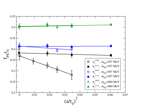
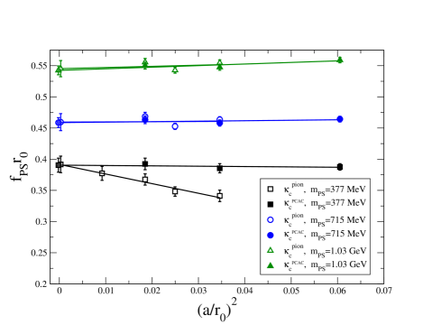
Figure 1: $r_{0}f_{\rm PS}$ as a function of $(a/r_{0})^{2}$ using the pion definition (open symbols) and the PCAC definition (filled symbols) of the critical mass; fits are performed with a linear function in $(a/r_{0})^{2}$ separately for each set.

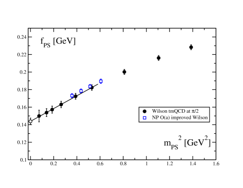
Figure 2: Continuum behaviour of $f_{\rm PS}$ (filled circles) as a function of the pseudoscalar mass squared (in physical units). We also plot the continuum limit obtained with non-perturbatively improved Wilson fermions (open squares) [19].

$\beta$	5.70	5.85	6.00	6.10	6.20	6.45
	$m_{\rm PS}a$ ($\kappa_{c}^{\rm pion}$)
$\mu_{1}a$	0.2455(23)	0.1682(26)	0.1385(66)	0.1129(41)	0.1004(27)	0.0720(28)
$\mu_{2}a$	0.3237(16)	0.2256(22)	0.1764(42)	0.1482(27)	0.1298(23)	0.0914(27)
$\mu_{3}a$	0.4434(11)	0.3122(19)	0.2373(32)	0.2030(21)	0.1768(17)
$\mu_{4}a$	0.6272(09)	0.4452(14)	0.3335(22)	0.2865(15)	0.2463(15)
$\mu_{5}a$	0.7767(09)	0.5535(12)	0.4134(17)	0.3534(13)	0.3037(13)
$\mu_{6}a$	0.9074(09)	0.6488(13)	0.4839(16)	0.4130(13)	0.3546(12)
$\mu_{7}a$	1.0255(08)	0.7358(12)	0.5491(14)	0.4676(12)	0.4021(11)
	$m_{\rm PS}a$ ($\kappa_{c}^{~\!\!\!{}_{\rm PCAC}}$)
$\mu_{1}a$	0.2323(18)	0.1640(23)	0.1217(66)		0.0934(24)
$\mu_{2}a$	0.3245(15)	0.2289(17)	0.1708(50)		0.1276(21)
$\mu_{3}a$	0.4598(12)	0.3232(13)	0.2396(33)		0.1779(18)
$\mu_{4}a$	0.6564(10)	0.4606(11)	0.3403(22)		0.2492(13)
$\mu_{5}a$	0.8114(10)	0.5701(10)	0.4214(17)		0.3071(12)
$\mu_{6}a$	0.9451(10)	0.6658(09)	0.4925(14)		0.3588(10)
$\mu_{7}a$	1.0647(09)	0.7530(09)	0.5579(14)		0.4062(09)
$\mu_{8}a$	0.3892(14)	0.2741(15)	0.2038(40)		0.1519(20)
$\mu_{9}a$	0.5678(11)	0.3984(12)	0.2948(26)		0.2160(16)

Table 3: Pseudoscalar meson masses $m_{\rm PS}a$ for all simulation points.

$\beta$	5.70	5.85	6.00	6.10	6.20	6.45
	$f_{\rm PS}a$ ($\kappa_{c}^{\rm pion}$)
$\mu_{1}a$	0.0986(10)	0.0782(13)	0.0516(17)	0.0466(14)	0.0437(13)	0.0329(13)
$\mu_{2}a$	0.1195(10)	0.0890(12)	0.0632(11)	0.0546(09)	0.0500(11)	0.0361(11)
$\mu_{3}a$	0.1418(11)	0.1003(12)	0.0740(09)	0.0623(08)	0.0562(10)
$\mu_{4}a$	0.1685(11)	0.1149(12)	0.0859(09)	0.0716(08)	0.0637(10)
$\mu_{5}a$	0.1902(11)	0.1273(13)	0.0949(09)	0.0790(08)	0.0698(09)
$\mu_{6}a$	0.2112(12)	0.1390(14)	0.1029(10)	0.0858(08)	0.0754(09)
$\mu_{7}a$	0.2320(13)	0.1501(14)	0.1104(10)	0.0919(09)	0.0806(09)
	$f_{\rm PS}a$ ($\kappa_{c}^{~\!\!\!{}_{\rm PCAC}}$)
$\mu_{1}a$	0.1267(14)	0.0894(14)	0.0689(27)		0.0512(16)
$\mu_{2}a$	0.1345(13)	0.0947(13)	0.0711(13)		0.0532(13)
$\mu_{3}a$	0.1472(12)	0.1025(12)	0.0763(10)		0.0567(10)
$\mu_{4}a$	0.1697(12)	0.1159(12)	0.0858(10)		0.0633(08)
$\mu_{5}a$	0.1914(13)	0.1284(11)	0.0944(10)		0.0694(08)
$\mu_{6}a$	0.2134(14)	0.1402(11)	0.1025(10)		0.0751(08)
$\mu_{7}a$	0.2358(15)	0.1518(11)	0.1100(10)		0.0803(08)
$\mu_{8}a$	0.1403(13)	0.0983(12)	0.0734(11)		0.0548(11)
$\mu_{9}a$	0.1589(12)	0.1095(12)	0.0813(10)		0.0601(09)

Table 4: Pseudoscalar meson decay constants $f_{\rm PS}a$ for all simulation points.

The vector meson mass shows, in comparison to $f_{\rm PS}$, larger statistical fluctuations at small masses. This fact, together with the considerably larger lattice artifacts which affect the values obtained with the pion definition of $\kappa_{c}$, makes the continuum extrapolation too difficult in this case. As a consequence we limit ourselves to present only the data obtained with the PCAC definition of $\kappa_{c}$. The vector meson mass has been extracted from the correlators eqs. (4) and (5) with local source and Jacobi-smeared sink [21]. We observe that the tensor correlator systematically shows smaller statistical fluctuations and thus we report in table 5 only results obtained from this correlator.

In fig. 3 we show the results for the vector meson mass as function of $(a/r_{0})^{2}$. Again, even for small pseudoscalar meson masses, the behaviour of the vector meson mass is almost flat in $(a/r_{0})^{2}$, indicating that $O(a^{2})$ lattice artefacts are also small for this quantity. We perform linear fits of these data as function of $(a/r_{0})^{2}$ which are represented by the lines in fig. 3. The continuum extrapolated values for the vector meson mass are presented in table 6 and in fig. 4. As a function of the pseudoscalar meson mass squared they show a linear behaviour without signs of q$\chi$PT artefacts. In fig. 4 we also plot the continuum values obtained with non-perturbatively improved Wilson fermions [19].

In table 6 the results of a linear extrapolation (performed with the seven smallest masses) of our data to the chiral limit are given. Moreover, we use this extrapolation to compute the values of $m_{\rho}$ and of $m_{K^{*}}$ (the latter in the $SU(3)$ symmetric limit). As already observed in quenched calculations where the scale is determined through $r_{0}$, these values turn out to be $10-15\%$ larger than the experimental values.

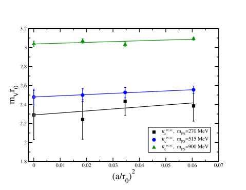
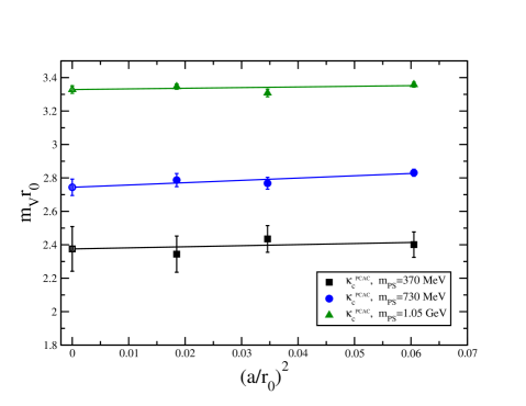
Figure 3: The vector meson mass as a function of $(a/r_{0})^{2}$ as obtained from the PCAC definition of the critical mass. We also show a linear fit in $(a/r_{0})^{2}$ of these quantity at fixed value of the charged pseudoscalar meson mass.

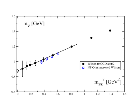
Figure 4: The continuum limit values of the vector meson mass (filled circles) as a function of the pseudoscalar meson mass squared. We also plot the continuum limit obtained with non-perturbatively improved Wilson fermions (open squares) [19].

$\beta$	5.70	5.85	6.00	6.20
	$m_{V}a$ ($\kappa_{c}^{~\!\!\!{}_{\rm PCAC}}$)
$\mu_{1}a$	0.716(67)	0.589(43)	0.458(30)	0.306(26)
$\mu_{2}a$	0.773(36)	0.591(19)	0.451(20)	0.317(20)
$\mu_{3}a$	0.854(20)	0.628(09)	0.467(12)	0.339(11)
$\mu_{4}a$	0.973(15)	0.701(05)	0.517(07)	0.378(05)
$\mu_{5}a$	1.076(11)	0.765(04)	0.560(06)	0.415(03)
$\mu_{6}a$	1.178(09)	0.834(03)	0.614(04)	0.452(02)
$\mu_{7}a$	1.277(08)	0.902(03)	0.666(03)	0.488(02)
$\mu_{8}a$	0.812(26)	0.606(13)	0.464(14)	0.327(16)
$\mu_{9}a$	0.919(14)	0.666(06)	0.494(08)	0.359(07)

Table 5: Vector meson masses $m_{V}a$ for all simulation points with the PCAC definition of $\kappa_{c}$.

As a last quantity, we computed the renormalisation constant $Z_{V}$ which is defined in eq. (9) and is to be obtained in the chiral limit. This renormalisation constant is expected to be equal, apart from lattice artifacts, to the one obtained for pure Wilson fermions. Also in this case we do not consider data obtained with the pion definition of $\kappa_{c}$. The reason is, as was shown in [4], that in this case the lattice artifacts affecting $Z_{V}$ become very large at small masses, thus preventing the possibility of performing a reliable extrapolation to the chiral limit. Using the PCAC definition of $\kappa_{c}$, lattice artifacts are well under control also at small quark masses (with the exception of $\beta=5.7$ where we prefer not to perform the chiral extrapolation). In fig. 5 we provide one example of $Z_{V}$ as a function of the quark mass. It turns out that $Z_{V}$ is to a good approximation linear in $(a\mu)^{2}$. In table 7 we report the values of $Z_{V}$ extrapolated to the chiral limit together with the results from standard perturbation theory (SPT)[22] (where the parameter of the expansion is $\alpha_{s}^{\rm SPT}=g_{0}^{2}/(4\pi)$, with $g_{0}^{2}=6/\beta$ the bare lattice coupling constant) and from boosted perturbation theory (BPT)[23] (where the parameter of the expansion is $\alpha_{s}^{\rm BPT}=\alpha_{s}^{\rm SPT}/{\cal P}$, with ${\cal P}=1/3\langle{\rm Re}\{{\rm{Tr}}P_{\mu\nu}\}\rangle$ the average value of the plaquette). Non-perturbative determinations with Wilson fermions using different methods are present in the literature for $\beta=6.0$ and give results in the range [0.57–0.74]. The spread is due to different $O(a)$ artifacts which affect the different determinations.

$m_{\rm PS}$ [GeV]	$f_{\rm PS}$ [GeV]	$m_{V}$ [GeV]
0.272	0.1500(66)	0.904(102)
0.372	0.1538(45)	0.937(53)
0.432	0.1572(40)	0.955(42)
0.514	0.1631(36)	0.978(33)
0.624	0.1724(33)	1.027(26)
0.728	0.1823(31)	1.083(19)
0.900	0.2002(29)	1.198(12)
1.051	0.2161(28)	1.313(09)
1.177	0.2283(28)	1.410(07)
0.0	0.1439(37)	0.876(25)
0.137	0.1452(37)	0.883(25)
0.495	0.1617(45)	0.973(27)

Table 6: $f_{\rm PS}$ and $m_{V}$ in the continuum with the PCAC definition of $\kappa_{c}$. The values in the last three rows are obtained from a linear fit on the smallest 6 masses (7 in the case of $m_{V}$) and correspond to: the values in the chiral limit (first row); $f_{\pi}$ and $m_{\rho}$ (second row); $f_{K}$ and $m_{K^{*}}$ in the $SU(3)$ symmetric limit (third row).

$\beta$	$Z_{V}$	$Z_{V}^{BPT}$	$Z_{V}^{SPT}$
5.85	0.5982(4)	0.69	0.82
6.0	0.6424(4)	0.71	0.83
6.2	0.6814(3)	0.73	0.83

Table 7: $Z_{V}$ from the PCVC relation (PCAC definition of $\kappa_{c}$) and comparison with standard perturbation theory (SPT) and boosted perturbation theory (BPT).

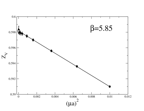
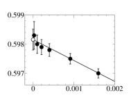
Figure 5: An example of the extrapolation of $Z_{V}$ to zero quark mass at $\beta=5.85$. The data show a linear behaviour in $(a\mu)^{2}$.

5 Conclusions

In this paper, we have explored the potential of Wilson twisted mass fermions to reach small quark masses and fine values of the lattice spacing. Using the PCAC definition of the critical mass the scaling region is found to start already at $\beta=5.85$, for the observables investigated here and for masses down to $270$ MeV. In fact, with this definition of the critical mass, correlators, apart from being automatically $O(a)$-improved, are only affected by $O(a^{2})$ discretisation errors which remain small in the region of masses that satisfy the (order of magnitude) inequality $\mu>a^{2}\Lambda_{QCD}^{3}$. In the case of the pion definition the $O(a^{2})$ effects are instead small only in the region $\mu>a\Lambda_{QCD}^{2}$ and, as observed in [4] and in the present work, may become quite relevant at masses in the range $250$-$450$ MeV and for the range of lattice spacings simulated here. In this case the scaling region starts, for masses down to 270 MeV, around $\beta=6.0$. However, at the two smallest quark masses, we included a point at $\beta=6.45$ in order to be sure that we can safely control the continuum limit extrapolation.

In the case of $f_{\rm PS}$ we have explicitly checked that both definitions of the critical mass lead independently to consistent values in the continuum limit. For further simulations, the PCAC definition of $\kappa_{c}$ is clearly preferable as it leads to considerably smaller lattice artifacts at small quark masses, allowing for an enlargement of the scaling region.

The results of this paper clearly reveal that Wilson twisted mass fermions allow for simulations at pseudoscalar meson masses of about $250$ MeV without running into problems with exceptional small eigenvalues or large lattice artefacts. This statement holds, when the PCAC definition of the critical mass is used. This is a very important lesson also for dynamical simulations, a lesson that we could only learn through the detailed quenched study performed here. In the dynamical case, however, small pseudoscalar meson masses are very difficult to simulate and further development of algorithms is still crucial. For example, modern variants of the Hybrid Monte Carlo algorithm allow to simulate pseudoscalar meson masses of about $380$ MeV [24, 25] without hitting the “Berlin Wall” [26, 27]. We therefore believe that by using these algorithmic techniques together with Wilson twisted mass fermions at maximal twist, realised by tuning the twist angle through the PCAC definition of the critical mass, it becomes realistic to address the small quark mass region in full, dynamical lattice QCD.

Appendix

Multiple mass solver for twisted mass fermions

In this appendix we show that within the Wilson twisted mass fermion formulation it is possible to apply the multiple mass solver (MMS) [28, 29, 30] method to the conjugate gradient (CG) algorithm. We will call this algorithm CG-M and give here the details of the implementation.

The advantage of the MMS is that it allows the computation of the solution of the following linear system

$$(A+\sigma)\;x-b=0$$ (10)

for several values of $\sigma$ simultaneously, using only as many matrix-vector operations as the solution of a single value of $\sigma$ requires.

We want to invert the Wilson twisted mass operator at a certain twisted mass $\mu_{0}$ obtaining automatically all the solutions for other twisted masses $\mu_{k}$ (with $|\mu_{k}|\geq|\mu_{0}|$). In the so called twisted basis the Wilson twisted mass operator is

$$D_{\rm tm}=D+i\mu_{k}\gamma_{5}\tau^{3},\qquad k=1,\ldots,N_{m}$$ (11)

where $D$ is the standard massive Wilson operator $D=D_{W}+m_{0}$ (see eq. (1) and (2)) and $N_{m}$ is the number of additional twisted masses. The operator can be splitted as

$$D_{\rm tm}=D_{\rm tm}^{(0)}+i(\mu_{k}-\mu_{0})\gamma_{5}\tau^{3},\qquad D_{\rm tm}^{(0)}=D+i\mu_{0}\gamma_{5}\tau^{3}\;.$$ (12)

The trivial observation is that

$$D_{\rm tm}D_{\rm tm}^{\dagger}=D_{\rm tm}^{(0)}D_{\rm tm}^{(0)\dagger}+\mu_{k}^{2}-\mu_{0}^{2}\;,$$ (13)

where we have used $\gamma_{5}D_{W}\gamma_{5}=D_{W}^{\dagger}$. Now clearly we have a shifted linear system $(A+\sigma_{k})x-b=0$ with $A=D_{\rm tm}^{(0)}D_{\rm tm}^{(0)\dagger}$ and $\sigma_{k}=\mu_{k}^{2}-\mu_{0}^{2}$. We describe now the CG-M algorithm in order to solve the problem $(A+\sigma_{k})x-b=0$. The lower index indicates the iteration steps of the solver, while the upper index $k$ refers to the shifted problem with $\sigma_{k}$.

$${\rm CG-M~{}~{}Algorithm}$$

$$x_{0}^{k}=0,r_{0}=p_{0}^{k}=b,\alpha_{-1}=\zeta_{-1}^{k}=\zeta_{0}^{k}=1,\beta_{0}^{k}=\beta_{0}=0$$

$${\rm for}~{}~{}i=0,1,2,\cdots$$

$$\quad\alpha_{n}={(r_{n},r_{n})\over(p_{n},Ap_{n})}$$

$$\quad\zeta_{n+1}^{k}={\zeta^{k}_{n}\alpha_{n-1}\over\alpha_{n}\beta_{n}(1-\frac{\zeta_{n}^{k}}{\zeta^{k}_{n-1}})+\alpha_{n-1}(1-\sigma_{k}\alpha_{n})}$$

$$\quad\alpha^{k}_{n}=\alpha_{n}{\zeta_{n+1}^{k}\over\zeta_{n}^{k}}$$

$$\quad x_{n+1}^{k}=x_{n}^{k}+\alpha_{n}^{k}p_{n}^{k}$$

$$\quad x_{n+1}=x_{n}+\alpha_{n}p_{n}$$

$$\quad r_{n+1}=r_{n}-\alpha_{n}Ap_{n}$$

$$\quad{\rm convergence~{}check}$$

$$\quad\beta_{n+1}={(r_{n+1},r_{n+1})\over(r_{n},r_{n})}$$

$$\quad p_{n+1}=r_{n+1}+\beta_{n+1}p_{n}$$

$$\quad\beta_{n+1}^{k}=\beta_{n+1}{\zeta_{n+1}^{k}\alpha_{n}^{k}\over\zeta_{n}^{k}\alpha_{n}}$$

$$\quad p_{n+1}^{k}=\zeta_{n+1}^{k}r_{n+1}+\beta_{n+1}^{k}p_{n}^{k}$$

$${\rm end~{}for}$$

We give here the algorithm explicitly again, since it has a different definition of $\zeta_{n+1}^{k}$ compared to the one of [30]. This version allows to avoid roundoff errors when $\sigma_{k}=\mu_{k}^{2}-\mu_{0}^{2}$ becomes too large.

We remind that when using a MMS the eventual preconditioning has to retain the shifted structure of the linear system. This means for example that it is not compatible with even-odd preconditioning.

References

- [1] ALPHA Collaboration, R. Frezzotti, P. A. Grassi, S. Sint, and P. Weisz, Lattice QCD with a chirally twisted mass term, JHEP 08 (2001) 058, [hep-lat/0101001].
- [2] R. Frezzotti and G. C. Rossi, Chirally improving Wilson fermions. I: O(a) improvement, JHEP 08 (2004) 007, [hep-lat/0306014].
- [3] L F Collaboration, K. Jansen, A. Shindler, C. Urbach, and I. Wetzorke, Scaling test for Wilson twisted mass QCD, Phys. Lett. B586 (2004) 432–438, [hep-lat/0312013].
- [4] L F Collaboration, W. Bietenholz et al., Going chiral: Overlap versus twisted mass fermions, JHEP 12 (2004) 044, [hep-lat/0411001].
- [5] L F Collaboration, K. Jansen, M. Papinutto, A. Shindler, C. Urbach, and I. Wetzorke, Light quarks with twisted mass fermions, Phys. Lett. B619 (2005) 184–191, [hep-lat/0503031].
- [6] A. M. Abdel-Rehim and R. Lewis, Twisted mass QCD for the pion electromagnetic form factor, Phys. Rev. D71 (2005) 014503, [hep-lat/0410047].
- [7] A. M. Abdel-Rehim, R. Lewis, and R. M. Woloshyn, Spectrum of quenched twisted mass lattice QCD at maximal twist, Phys. Rev. D71 (2005) 094505, [hep-lat/0503007].
- [8] F. Farchioni et al., Twisted mass quarks and the phase structure of lattice QCD, Eur. Phys. J. C39 (2005) 421–433, [hep-lat/0406039].
- [9] F. Farchioni et al., Exploring the phase structure of lattice QCD with twisted mass quarks, Nucl. Phys. Proc. Suppl. 140 (2005) 240–245, [hep-lat/0409098].
- [10] F. Farchioni et al., The phase structure of lattice QCD with Wilson quarks and renormalization group improved gluons, accepted for publication in Eur. Phys. J. C (2005) [hep-lat/0410031].
- [11] E.-M. Ilgenfritz, W. Kerler, M. Müller-Preußker, A. Sternbeck, and H. Stüben, A numerical reinvestigation of the Aoki phase with N(f) = 2 Wilson fermions at zero temperature, Phys. Rev. D69 (2004) 074511, [hep-lat/0309057].
- [12] A. Sternbeck, E.-M. Ilgenfritz, W. Kerler, M. Müller-Preußker, and H. Stüben, The Aoki phase for N(f) = 2 Wilson fermions revisited, Nucl. Phys. Proc. Suppl. 129 (2004) 898–900, [hep-lat/0309059].
- [13] L F Collaboration, W. Bietenholz et al., Comparison between overlap and twisted mass fermions towards the chiral limit, Nucl. Phys. Proc. Suppl. 140 (2005) 683–685, [hep-lat/0409109].
- [14] S. Aoki and O. Bar, Twisted-mass QCD, O(a) improvement and Wilson chiral perturbation theory, Phys. Rev. D70 (2004) 116011, [hep-lat/0409006].
- [15] S. R. Sharpe and J. M. S. Wu, Twisted mass chiral perturbation theory at next-to-leading order, Phys. Rev. D71 (2005) 074501, [hep-lat/0411021].
- [16] R. Frezzotti, G. Martinelli, M. Papinutto, and G. C. Rossi, Reducing cutoff effects in maximally twisted lattice QCD close to the chiral limit, hep-lat/0503034.
- [17] R. Frezzotti and S. Sint, Some remarks on O(a) improved twisted mass QCD, Nucl. Phys. Proc. Suppl. 106 (2002) 814–816, [hep-lat/0110140].
- [18] M. Della Morte, R. Frezzotti, and J. Heitger, Quenched twisted mass QCD at small quark masses and in large volume, Nucl. Phys. Proc. Suppl. 106 (2002) 260–262, [hep-lat/0110166].
- [19] ALPHA Collaboration, J. Garden, J. Heitger, R. Sommer, and H. Wittig, Precision computation of the strange quark’s mass in quenched QCD, Nucl. Phys. B571 (2000) 237–256, [hep-lat/9906013].
- [20] ALPHA Collaboration, J. Heitger, R. Sommer, and H. Wittig, Effective chiral lagrangians and lattice QCD, Nucl. Phys. B588 (2000) 377–399, [hep-lat/0006026]. and references therein.
- [21] UKQCD Collaboration, C. R. Allton et al., Gauge invariant smearing and matrix correlators using Wilson fermions at beta = 6.2, Phys. Rev. D47 (1993) 5128–5137, [hep-lat/9303009].
- [22] G. Martinelli and Y.-C. Zhang, The connection between local operators on the lattice and in the continuum and its relation to meson decay constants, Phys. Lett. B123 (1983) 433.
- [23] G. P. Lepage and P. B. Mackenzie, On the viability of lattice perturbation theory, Phys. Rev. D48 (1993) 2250–2264, [hep-lat/9209022].
- [24] C. Urbach, K. Jansen, A. Shindler, and U. Wenger, HMC algorithm with multiple time scale integration and mass preconditioning, hep-lat/0506011.
- [25] M. Lüscher, Schwarz-preconditioned HMC algorithm for two-flavour lattice QCD, Comput. Phys. Commun. 165 (2005) 199, [hep-lat/0409106].
- [26] K. Jansen, Actions for dynamical fermion simulations: Are we ready to go?, Nucl. Phys. Proc. Suppl. 129 (2004) 3–16, [hep-lat/0311039].
- [27] C. Bernard et al., Panel discussion on the cost of dynamical quark simulations, Nucl. Phys. Proc. Suppl. 106 (2002) 199–205.
- [28] R. Freund in Numerical Linear Algebra, L. Reichel, A. Ruttan and R.S. Varga (eds.) (1993) p. 101.
- [29] U. Glässner et al., How to compute Green’s functions for entire mass trajectories within Krylov solvers, hep-lat/9605008.
- [30] B. Jegerlehner, Multiple mass solvers, Nucl. Phys. Proc. Suppl. 63 (1998) 958–960, [hep-lat/9708029, hep-lat/9612014].