Abstract

We investigate the overlap operator with a UV filtered Wilson kernel. The filtering leads to a better localization of the operator even on coarse lattices and with the untuned choice $\rho\!=\!1$. Furthermore, the axial-vector renormalization constant $Z_{A}$ is much closer to 1, reducing the mismatch with perturbation theory. We show that all these features persist over a wide range of couplings and that the details of filtering prove immaterial. We investigate the properties of the kernel spectrum and find that the kernel non-normality is reduced. As a side effect we observe that for certain applications of the filtered overlap a speed-up factor of 2-4 can be achieved.

1 Introduction

From a theoretical viewpoint the ascent of “overlap” fermions [3, 4, 5], i.e. fermions which at zero quark mass satisfy the Ginsparg Wilson (GW) relation [6] ($\rho$ is a parameter that will be specified later)

$$\gamma_{5}D+D\hat{\gamma}_{5}=0,\qquad\hat{\gamma}_{5}=\gamma_{5}(1-{1\over\rho}D)$$ (1)

and thus realize a lattice version of the continuum chiral symmetry [7]

$$\delta\psi=\hat{\gamma}_{5}\psi,\qquad\delta\overline{\psi}=\overline{\psi}\gamma_{5}$$ (2)

together with an index theorem [8, 9], represents a major breakthrough in the field of non-perturbative studies of QCD. We know how to discretize fermions in a way that preserves the relevant symmetries: $(i)$ gauge invariance, $(ii)$ flavor symmetry, and $(iii$) chiral invariance. Unfortunately, from a practical viewpoint the usefulness of this concept is limited by the fact that the overlap tends to be one to two orders of magnitude more expensive, in terms of CPU time, than a standard Wilson Dirac operator.

In this paper we study a variant of the overlap operator which makes use of a UV filtered Wilson kernel. Here, the “filtering” refers to replacing the original (“thin”) links of the gauge configuration in the standard definition of the Wilson kernel by “thick” links obtained through APE [10] or HYP [11] smearing. This is a legal change of discretization as long as one keeps the iteration level and smearing parameters fixed all the way down to the continuum, since the “thick” links transform under a local gauge transformation in the same way as the “thin” links; it should be seen as a modification of the operator and not of the gauge background. Such filtering has been used in the context of staggered quarks, where it has been found to reduce UV fluctuations, in particular taste changing interactions due to highly virtual gluons [12]. In Ref. [13] filtered staggered quarks were compared against overlap quarks (where the filtered version was merely considered for completeness), and it was observed that a single filtering step may speed up the forward application of the overlap operator $D_{\mathrm{ov}}$ on a source vector by a factor 2-4, depending on the gauge background. This was seen to come through a reduction of the degree of the Chebychev polynomial needed to approximate the inverse square root or sign function in the definition of the massless overlap [5]

$$aD_{\mathrm{ov}}=\rho\Big{[}1+D_{\mathrm{W},-\rho}(D_{\mathrm{W},-\rho}^{\dagger}D_{\mathrm{W},-\rho})^{-1/2}\Big{]}=\rho\Big{[}1+\gamma_{5}\,\mathrm{sign}(a\gamma_{5}D_{\mathrm{W},-\rho})\Big{]}$$ (3)

with $D_{\mathrm{W},-\rho}\!=\!D_{\mathrm{W}}-\!\rho/a$ the Wilson operator at negative mass $-\rho/a$. However, what matters in view of most phenomenological applications is the performance of the massive operator (bare quark mass $m$)

$$D_{\mathrm{ov},m}=(1\!-{am\over 2\rho})D_{\mathrm{ov}}+m$$ (4)

in the process of calculating a given physical observable to a pre-defined accuracy. In other words the total CPU time spent depends on:

1. The number of forward applications of the shifted Wilson operator $D_{\mathrm{W},-\rho}$ (or, generally speaking, of the kernel) needed to construct the massless overlap operator (3).

2. The number of iterations spent on inverting the so-constructed massive operator (4) for a given renormalized quark mass (or a given $M_{\pi}^{2}$).

3. The number of gauge backgrounds needed to reach a pre-defined statistical accuracy of the desired observable at a given lattice spacing $a$.

4. The lattice spacing needed to enter the scaling window.

The main emphasis of this paper will be on point 1; in particular we attempt to give an understanding of the observed speedup in terms of the spectral properties of the underlying hermitean (shifted) Wilson operator $H_{\mathrm{W}}\!=\!\gamma_{5}D_{\mathrm{W},-\rho}$. At first sight it might seem that point 2 does not need to be considered at all. At fixed bare mass $m$ and fixed $\rho$ the filtered and the unfiltered overlap do not differ on this point, since the number of forward applications of $D_{\mathrm{ov},m}$ to get a column of the inverse depends only on its condition number, and that is $2\rho/m$ for either variety. As we shall see, the optimum $\rho$ (w.r.t. locality) gets reduced through filtering whereas $Z_{m}\!=\!Z_{S}^{-1}\!=\!Z_{P}^{-1}$ increases and this means that in the filtered case one has to use a smaller bare mass to work at a fixed physical $m^{\mathrm{ren}}\!=\!Z_{m}m$. These two aspects tend to compensate, and as a result there is little net effect on point 2 from filtering. Whether in points 3 and 4 filtering brings further savings is not clear, but we plan to address this issue in the future.

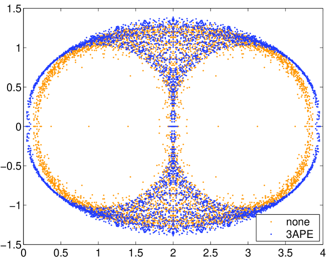
Figure 1: Eigenvalue spectra of $D_{\mathrm{W}}$ with $\kappa\!=\!\kappa_{\mathrm{crit}}^{\mathrm{tree}}\!=\!0.25$ in the quenched Schwinger model ($16^{2}$, $\beta\!=\!3.2$, 10 configurations) without filtering and after 3 steps with $\alpha\!=\!0.5$ (i.e. equal weight to the original link and the staple, see [14] for details; in 2D APE involves already the full hypercube). Filtering depletes the “bellies”, makes the physical (leftmost) branch narrower and shifts it to the left.

Let us try to obtain a first understanding of the effect of filtering in terms of the spectrum of the underlying (non-hermitean) Wilson operator. We are going to compute all eigenvalues, and to avoid spending too much CPU time on this illustration, we shall do this in 2D, but it is clear that the conceptual issue is – mutatis mutandis – the same as in 4D. In $d$ dimensions the Wilson Dirac operator has $d\!+\!1$ branches, and the respective flavor multiplicities are

$${d\choose 0}\;,\;{d\choose 1}\;,\;\;...\;\;,\;{d\choose d}\;.$$ (5)

Thus in 2D the Wilson operator has 3 branches with multiplicities 1,2,1, while in 4D it has 5 branches with multiplicities 1,4,6,4,1, respectively. Fig. 1 shows the complete spectrum of $D_{\mathrm{W}}$ with the hopping parameter fixed at its tree-level critical value, $\kappa\!=\!0.25$, on 10 configurations of size $16^{2}$ at $\beta\!=\!3.2$ in the quenched Schwinger model. Besides the “thin” link operator also its UV filtered descendent is shown. In terms of the kernel spectrum the filtering is seen to have the following effects:

1. The two/four “bellies” are depleted — in particular exactly real modes which cannot be assigned in a unique way to one of the three/five branches are severely suppressed.

2. The horizontal scatter of any of the three/five branches diminishes.

3. The additive mass renormalization of the physical (leftmost) branch is substantially reduced.

If one were to ignore the kernel non-normality (we shall come back to this point), the spectrum of $D_{\mathrm{W}}$ could be linked, on a mode-by-mode basis, to the one of $D_{\mathrm{W},-\rho}^{\dagger}D_{\mathrm{W},-\rho}$, $H_{\mathrm{W}}\!=\!\gamma_{5}D_{\mathrm{W},-\rho}$ and $D_{\mathrm{ov}}$. Then the first observation above (the reluctance of the filtered eigenvalues to show up near the projection point $\rho$) simply means that the effect of filtering on the spectrum of $H_{\mathrm{W}}$ is to deplete the vicinity of the origin by pushing the eigenvalues further towards the ends of the interval $[-2d\!+\!1,2d\!-\!1]$. In spite of the caveat mentioned, the thinning effect that (any kind of) smearing has on the spectrum of $H_{\mathrm{W}}$ near zero is indeed the reason for the speedup in point 1 above. A bigger interval $[0,\epsilon^{2}[$ or $]-\!\epsilon,\epsilon[$ that does not need to be covered by the polynomial/rational approximation to the $1/\!\sqrt{.}$ or $\mathrm{sign}(.)$ function translates into a lower degree and thus into fewer forward applications of the kernel operator.

In the remainder of this article we shall address the spectral properties of $H_{\mathrm{W}}$ in more detail (Sec. 2), and show that (a reasonable amount of) filtering does not degrade the locality properties of $D_{\mathrm{ov}}$, but rather makes the overlap operator more local (Sec. 3). We continue with an explicit demonstration that the kernel non-normality gets reduced by filtering (Sec. 4). We add some observations relevant to phenomenological applications of the filtered overlap; in particular $Z_{A}$ is shown to be much closer to the tree-level value 1 than for the unfiltered variety (Sec. 5). We rate this as a sign that perturbation theory might work far better for the filtered overlap. We make an attempt to compare our simple filtering recipe against other approaches (Sec. 6). Finally, the appendix contains spectral data which suggest that the spectral density of $H_{\mathrm{W}}$ at the origin is non-zero for any $\beta$ and any filtering level.

We shall use pure gauge backgrounds and set the scale through the Sommer parameter $r_{0}$ [15]. We choose the Wilson gauge action, and since $r_{0}(\beta)$ is known [16] it is easy to select $\beta$ values such that the resulting lattices are matched, i.e. have fixed spatial size $L\!\simeq\!1.5\,\mathrm{fm}$, with the resolution varying by a factor 3 from the coarsest to the finest lattice – see Tab. 1 for details. Henceforth we set $a\!=\!1$.

$\beta$	$5.66$	$5.84$	$6.00$	$6.26$
geometry	$8^{4}$	$12^{4}$	$16^{4}$	$24^{4}$
geometry	$8^{3}\!\times\!16$	$12^{3}\!\times\!24$	$16^{3}\!\times\!32$	—

Table 1: Survey of matched 4D couplings and geometries with fixed $L/r_{0}\!\approx\!3$, according to the interpolation formula of Ref. [16]. The first coupling is slightly out of bound (see discussion in [16]).

2 Speedup and kernel spectrum

In a quenched simulation the overhead, in terms of CPU time, of overlap versus Wilson quarks comes in the first place from the polynomial or rational approximation to the $1/\!\sqrt{.}$ or $\mathrm{sign}(.)$ function in (3). Let us assume that the lowest eigenvalue of the unfiltered $|H_{\mathrm{W}}|$ is $0.14$ while the highest eigenvalue takes the free field value 7. This leads to the task to construct a polynomial/rational approximation of the inverse square root over the range $[\epsilon^{2},1]$ with $\epsilon\!=\!0.02$ the inverse condition number of $|H_{\mathrm{W}}|$. Modest filtering will lift the lowest eigenvalue to something like $0.49$, while the largest eigenvalue is almost invariant. Then the task is to construct the approximation over the range $[\tilde{\epsilon}^{2},1]$ with $\tilde{\epsilon}\!=\!0.07$ the filtered inverse condition number. The lower bound increasing from $0.0004$ to $0.0049$ means that one gets away with a smaller overall polynomial degree or an increased minimum root of the denominator polynomial. Therefore, the filtered overlap requires fewer forward applications of $D_{\mathrm{W},-\rho}^{\dagger}D_{\mathrm{W},-\rho}$ and this is how the savings on CPU time in point 1 above come about. In the remainder of this section we will elaborate on this statement, replace the fictitious numbers by actual figures from real simulations and see that the conclusion remains unchanged.

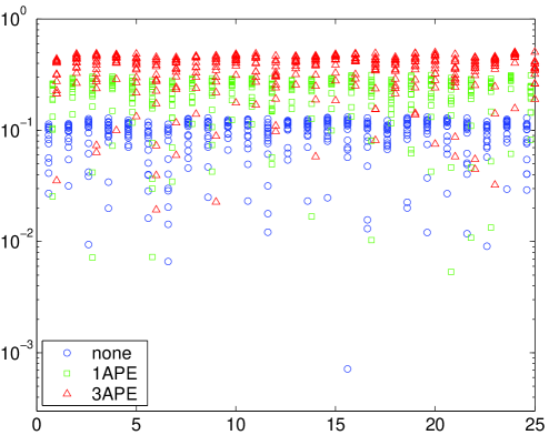
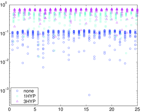
Figure 2: Sequence of the lowest 15 eigenvalues of $|H_{\mathrm{W}}|$ on 25 configurations at $\beta\!=\!6.0$ without filtering and after 1,3 steps of APE (left) or HYP (right) filtering. Throughout $\rho\!=\!1$.

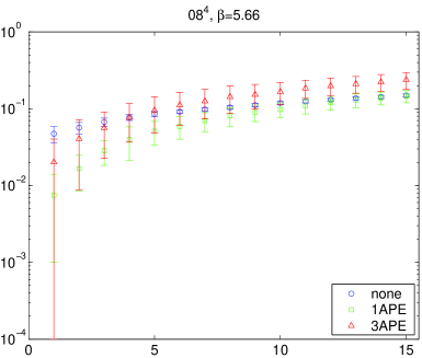
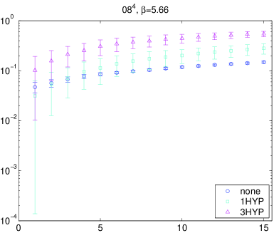
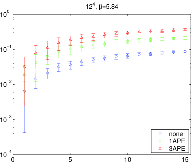
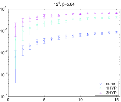
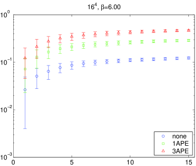
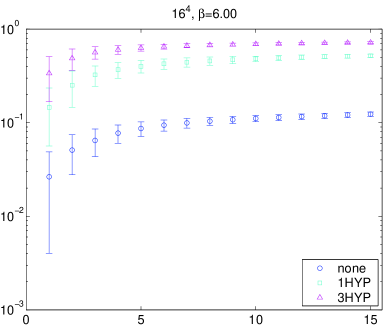
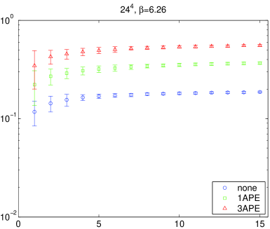
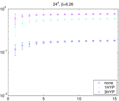
Figure 3: Mean and standard deviation ($\beta\!=\!5.66,5.84,6.00,6.26$, from top to bottom) of the 15 lowest eigenvalues of $|H_{\mathrm{W}}|$ at $\rho\!=\!1$ in semi-logarithmic form with 0,1,3 steps of APE or HYP filtering.

Fig. 2 shows, as an illustration, the 15 lowest eigenvalues [17] of $|H_{\mathrm{W}}|$ on 25 configurations at $\beta\!=\!6.0$, without filtering and after 1,3 steps of APE or HYP smoothing. The filtering increases the upper end of the band of eigenvalues shown. In fact, just this upper end matters in terms of CPU time, since in practice one projects out the lowest few modes [18] and constructs the function in (3) over the relevant spectral range of $|H_{\mathrm{W}}|$ on the subspace orthogonal to these modes. Hence the sequence of the 15th eigenvalue represents the relevant quantity, if 14 modes are treated exactly, and this band gets lifted by filtering. Evidently, a single APE step is less efficient than a single HYP step, and adding two more steps lifts the 15th eigenvalue further, but the lifting factor is no more as large as it was in the first step. Here and below we use the parameters $\alpha_{\mathrm{APE}}\!=\!0.5$, $\alpha_{\mathrm{HYP}}\!=\!(0.75,0.6,0.3)$ [11] (for details of the $SU(3)$ projection see e.g. [19] or the appendix of [20]) and, unless stated otherwise, $\rho\!=\!1$.

$\beta$	$5.66$	$5.84$	$6.00$	$6.00\;(\rho=1.4)$	$6.26$
none	0.149(02)	0.087(2)	0.123(1)	0.222(3)	0.187(1)
1 APE	0.146(05)	0.213(4)	0.290(2)	0.343(5)	0.368(2)
3 APE	0.237(12)	0.364(6)	0.469(2)	0.547(7)	0.557(2)
1 HYP	0.281(14)	0.419(7)	0.519(2)	0.618(5)	0.597(2)
3 HYP	0.548(14)	0.653(5)	0.717(1)	0.639(1)	0.770(1)

Table 2: Start of the “bulk” part of the eigenvalue spectrum of the shifted hermitean Wilson operator $|H_{\mathrm{W}}|$ without filtering and after one or three APE or HYP steps. We use the mean of the 15th-smallest eigenvalue to define the “bulk” edge. Unless indicated otherwise, the numbers refer to the case $\rho\!=\!1$.

Fig. 3 shows the mean and the standard deviation of the 15 lowest eigenvalues of $|H_{\mathrm{W}}|$, with our standard filtering options (none, 1 APE, 3 APE, 1 HYP, 3 HYP). In this logarithmic representation it is easy to see that (apart from the coarsest lattice which represents a special case discussed in App. A) all 15 eigenvalues get lifted, at a given coupling, by virtually the same factor. Specifically, the 15th eigenvalue gets multiplied by $\lambda_{\mathrm{1\,HYP}}/\lambda_{\mathrm{none}}\!=\!4.8,4.2,3.2$ at $\beta\!=\!5.84,6.00,6.26$. Thus the lifting effect that filtering has on the “bulk” part of the $|H_{\mathrm{W}}|$ spectrum diminishes somewhat towards the continuum, but for accessible couplings it remains substantial. Details of the ensemble average of the 15th eigenvalue are collected in Tab. 2. The second observation is that the bands become flatter at large $\beta$, hence the onset of the “bulk” becomes a less ambiguous concept at weaker coupling. Had we chosen the 10th or 20th mode to define the “bulk edge” instead of the 15th, this would cause a small change at $\beta\!=\!6.26$, but it would make a substantial difference at the smallest $\beta$ shown.

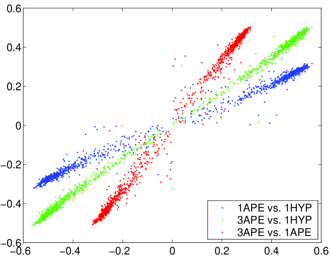
Figure 4: Correlation of the 15 eigenvalues closest to zero of $H_{\mathrm{W}}$ with various filtering options at $\beta\!=\!6.0$.

A point of theoretical interest is whether the low-lying eigenvalues of the (shifted) hermitean Wilson operator $H_{\mathrm{W}}$ are correlated, between different smearing levels, just as the low-lying eigenvalues of the final $D_{\mathrm{ov}}$ were found to be correlated for large enough $\beta$ [13]. Fig. 4 shows that this is almost true – the eigenvalues correlate if they are sufficiently large in absolute magnitude, but the correlation weakens closer to the origin. Here, a technical issue comes along. Ideally, one would pair the eigenvalues by considering a smooth interpolation between the two filtering recipes. Changes in topology (as seen by the overlap operator) would then be evident as stray points in quadrants 2 or 4. However, since we just know the eigenvalues shown we decided to pair them starting from 0. Now there are no points in quadrants 2 or 4 by definition and changes in topology manifest themselves through a reduced correlation of the few lowest eigenvalues in absolute magnitude. Such topology changes are expected to occur with an $O(a^{2})$ re-definition of the overlap operator, e.g. by changing the filtering or $\rho$ [13].

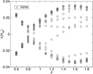
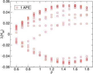
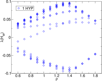
Figure 5: Eigenvalue flows of $H_{\mathrm{W}}$ with three filterings (none, 1 APE, 1 HYP) on one $16^{4}$ configuration.

A similar conclusion is drawn from the flow of eigenvalues $H_{\mathrm{W}}$ as shown in Fig. 5 for one $16^{4}$ configuration. One effect of filtering is to stretch the whole scenery in the vertical direction (note the vertical scale). Filtering also shifts the entire eigenvalue flow to the left which is consistent with the reduction of the additive mass renormalization of the kernel operator as discussed in the introduction. Note that there is, from a conceptual viewpoint, no reason to prefer one filtering level over any other one; what we see is just a manifestation of the $O(a^{2})$ ambiguity of the overlap operator [13].

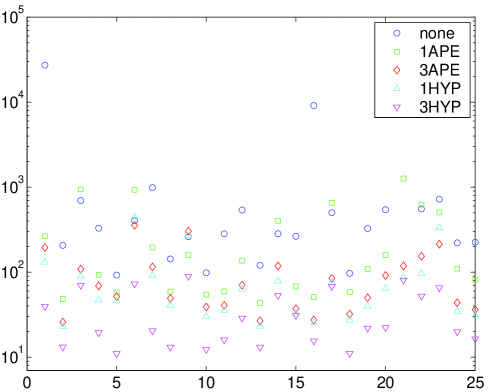
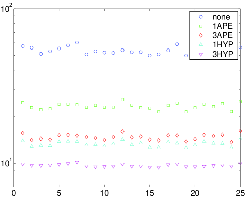
Figure 6: Condition number of $|H_{\mathrm{W}}|$ on 25 configurations at $\beta\!=\!6.0$ without projection (left) and with 14 modes handled exactly (right), after 0,1,3 steps of APE or HYP filtering.

$\beta$	$5.66$	$5.84$	$6.00$	$6.00\;(\rho=1.4)$	$6.26$
none	43.5(04)	75.2(15)	53.2(4)	27.9(4)	35.3(2)
1 APE	47.2(18)	31.8(06)	23.4(2)	18.6(3)	18.5(1)
3 APE	30.5(17)	19.0(03)	14.7(1)	11.9(2)	12.4(1)
1 HYP	25.7(14)	16.5(03)	13.3(1)	10.5(1)	11.6(1)
3 HYP	12.8(04)	10.6(01)	9.69(3)	10.2(1)	9.04(2)

Table 3: Mean condition number $1/\epsilon$ of $|H_{\mathrm{W}}|$ at $\rho\!=\!1$ after projecting the 14 lowest eigenmodes.

To assess the CPU time needed for the massless overlap, the behavior of the “bulk edge” of the $|H_{\mathrm{W}}|$ spectrum is one ingredient. What really matters is the condition number, thus we need to study the largest eigenvalue, too. From the naive discussion around Fig. 1 in the introduction one expects that filtering barely affects the largest eigenvalue of $|H_{\mathrm{W}}|$. It turns out that this is indeed true, for instance at $\beta\!=\!6.0$ a single HYP filtering step lifts it from $6.55(1)$ to $6.88(1)$. Hence, filtering has an overall beneficial effect on the condition number as illustrated in Fig. 6. Without projection the condition number fluctuates wildly and occasionally it may increase through filtering (i.e. the lowest eigenvalue decreases, cf. Fig. 2) but after projecting 14 eigenmodes this never occurs. The bottom line is that the combination of filtering and projection reduces the condition number much more vigorously than either one alone could do. Average condition numbers after projecting out 14 eigenmodes are collected in Tab. 3 (regarding the first entry, cf. App. A). As a side remark we note that the horizontal increase to the left explains why in a fixed physical volume simulating unfiltered overlap quarks on a coarse lattice is not so much cheaper than on a fine one; for the filtered version this penalty is reduced.

We have also studied the condition number of $|H_{\mathrm{W}}|$ as a function of the parameter $\rho$. With and without filtering the minimum is rather shallow and at a $\rho$ value above $1$. Since in the free case

$$\epsilon=\left\{\begin{array}[]{ll}\rho/(8\!-\!\rho)&\mathrm{for}\;0\!<\!\rho\!\leq\!1\\ (2\!-\!\rho)/(8\!-\!\rho)&\mathrm{for}\;1\!\leq\!\rho\!<\!2\end{array}\right.$$ (6)

we expect that larger $\beta$ values will further drive the minimum location towards $\rho\!=\!1$.

The last step is to convert the reduced condition number, brought by the filtering, of $|H_{\mathrm{W}}|$ on the subspace orthogonal to the lowest 14 modes into a lower degree of the polynomial/rational approximation of the $1/\!\sqrt{.}$ function in (3) and thus into actual savings of CPU time in step 1 of the introduction.

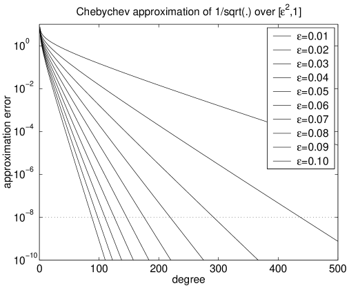
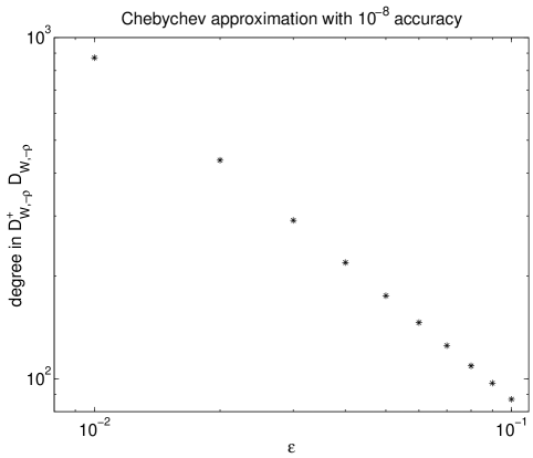
Figure 7: Accuracy of the Chebychev approximation of $(.)^{-1/2}$ over the interval $[\epsilon^{2},1]$ versus polynomial degree (left) and the degree (number of forward applications of $D_{\mathrm{W},-\rho}^{\dagger}D_{\mathrm{W},-\rho}$) needed to reach absolute accuracy $10^{-8}$ versus the inverse condition number $\epsilon$ of the shifted hermitean Wilson operator $|H_{\mathrm{W}}|$.

The precise speedup factor depends on the implementation of the massless overlap operator (3). For definiteness let us consider the approximation of the inverse square root over the range $[\epsilon^{2},1]$ through Chebychev polynomials [18]. Fig. 7 shows on the l.h.s. for a few inverse condition numbers $\epsilon$ of $|H_{\mathrm{W}}|$ the well known exponential fall-off pattern of the truncation error of the Chebychev approximation versus the number of applications of $H_{\mathrm{W}}^{2}\!=\!D_{\mathrm{W},-\rho}^{\dagger}D_{\mathrm{W},-\rho}$. What matters for our purpose is the dependence of the polynomial degree required to reach a fixed minimax accuracy – say $\delta\!=\!10^{-8}$ over the full approximation range – on $\epsilon$. As is evident from the r.h.s. of that figure, the relation

$$\mathrm{degree}\propto{\epsilon^{-1}}$$ (7)

holds in good approximation. Thus, from (7) and a look at Tab. 3 one predicts that at $\beta\!=\!6.0$ and $\rho\!=\!1$ a single HYP step will speed up the construction of the overlap (on average) by a factor $53.2/13.3\!=\!4.00$, and this is in good agreement with what we find in actual runs (see Fig. 8). On a coarser lattice this factor would be somewhat larger ($4.56$ at $\beta\!=\!5.84$) while on a finer lattice it tends to decrease ($3.04$ at $\beta\!=\!6.26$), but it certainly remains substantial at all accessible couplings.

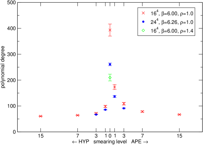
Figure 8: Mean and standard deviation of the Chebychev polynomial degree used to achieve a minimax accuracy of $10^{-8}$. At $\beta\!=\!6.0$ and $\rho\!=\!1$, a single HYP step results in a speedup by a factor $\sim\!4$ for the massless overlap operator. Comparing to the situation with $\rho\!=\!1.4$ and no filtering the factor is $\sim\!2$.

To approximate the inverse square root or sign function over the relevant range, two main strategies are found in the literature. Polynomial [21, 22, 18] and rational [22, 23] representations have been tried. We have concentrated on the Chebychev variant, since this one is efficient and easy to implement. It goes without saying that the lifting effect on the bulk of the $|\gamma_{5}D_{\mathrm{kern}}|$ eigenvalues translates into similar savings on CPU time in step 1 of the introduction, if another representation is used. For instance, in the rational approach it is the increase of the smallest zero of the denominator polynomial that lets one get away with fewer iterations in the inner multishift CG.

For five dimensional variants of the overlap operator [24, 25, 26, 27, 28], in particular the domain wall formulation, the computational gain comes from the reduction of the extent of the fifth dimension needed to reach a given residual mass. What we would like to stress here is simply that our proposal to replace the “thin” links by “thick” links is generically useful for any kind of overlap variant.

3 Locality

It has been shown [29] that the overlap operator cannot be ultralocal, as opposed to the Wilson operator where $D_{\mathrm{W}}(x,y)\!=\!0$ for $||x\!-\!y||_{1}\!>\!1$. To guarantee the universality of the underlying field theory and hence to obtain the correct continuum limit it is sufficient to have an operator with

$$D_{\mathrm{ov}}(x,y)\propto\exp(-\nu||x-y||)\qquad\mathrm{for}\quad||x-y||\gg 1$$ (8)

where the localization $\nu$ is of the order of the cut-off, i.e. $\nu\!=\!O(1)$ [in lattice units]. In practice, for a given lattice spacing the condition (8) gives an upper bound on any physical mass that one can extract, and it is therefore crucial to have an operator as local as possible, i.e. with a maximal $\nu$. In [30] it has been demonstrated that the standard overlap operator indeed obeys (8). It is clear that their proof goes through for our filtered variant, but it is open in which way the localization $\nu$ is influenced. Naively, one might think that the locality will deteriorate, since the original links entering the covariant derivative of the filtered kernel spread over a larger volume. As first observed by Kovacs [31], the filtered overlap turns out to be even more local than the standard one and this is achieved without tuning $\rho$.

Figure 9: Localization of the overlap at $\beta\!=\!6.0$ without filtering and after 1 HYP step, for $\rho\!=\!1.0$ and $\rho\!=\!1.4$. A single HYP step proves more efficient than optimizing $\rho$. Filtering and $\rho\!>\!1$ should not be combined; for the filtered operator the untuned choice $\rho\!=\!1$ is reasonable (but still not optimal).

In Fig. 9 we plot the localization of $D_{\mathrm{ov}}$ at $\beta\!=\!6.0$ with two projection parameters ($\rho\!=\!1.0,1.4$) and two filtering options (none, 1 HYP). The ordinate is the maximum over the 2-norm of $D_{\mathrm{ov}}\eta$ at $x$ with $\eta$ a normalized $\delta$-peak source vector at the point $y$ in the lattice, the abscissa is the “taxi driver” distance $d_{1}\!=\!||x\!-\!y||_{1}$ to the location of the $\delta$-peak, i.e. we plot the function

$$f(d_{1})=\mathrm{sup}\Big{\{}||(D_{\mathrm{ov}}\eta)(x)||_{2}\;\Big{|}\;||x\!-\!y||_{1}\!=\!d_{1}\Big{\}}$$ (9)

versus $d_{1}$, as first studied in [30]. Comparing the two unfiltered operators (black/dark diamonds and crosses) one finds their result reproduced that (at this $\beta$) adjusting $\rho$ to a value around $1.4$ lets $f(d_{1})$ fall off steeper than with the value $1.0$ which is the canonical choice in view of the spectrum of the Wilson operator sufficiently close to the continuum (cf. Fig. 1). The interesting observation is that a single HYP step together with $\rho\!=\!1.0$ (red/light squares) results in an even steeper descent than the unfiltered version with $\rho\!=\!1.4$ (which was chosen to nearly optimize the locality of the unfiltered operator). The last curve shown (red/light pluses) indicates that one should not attempt to combine the filtering with a $\rho$ value that would be optimal for the unfiltered operator.

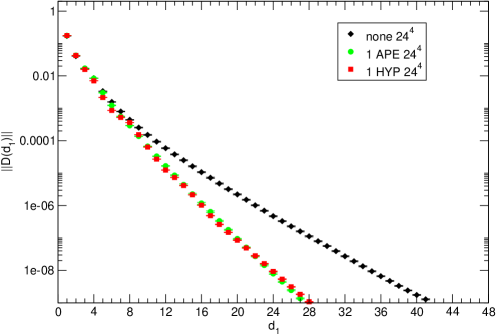
Figure 10: Localization of the unfiltered overlap and of the versions with one APE or HYP step. The data are for the matched ensembles ($8^{4}$ at $\beta\!=\!5.66$, $12^{4}$ at $\beta\!=\!5.84$, $16^{4}$ at $\beta\!=\!6.00$, $24^{4}$ at $\beta\!=\!6.26$) and $\rho\!=\!1$ throughout. On sufficiently fine lattices the choice of smearing proves irrelevant.

An obvious question is whether filtering remains useful on fine lattices. Fig. 10 shows the fall-off at four couplings with no smearing, 1 APE and 1 HYP step, with $\rho\!=\!1$ fixed. On the coarsest lattice smearing alters the locality just modestly, on the two intermediate ones ($\beta\!=\!5.84,6.00$) the locality gets substantially improved, with HYP doing a better job than APE. On the finest lattice, the improvement is still sizable, but there is almost no difference among the two filtering recipes. At this coupling further smearing steps would then diminish the locality. The localization measured with the definition (29) [which we use for technical reasons discussed below] is summarized in Tab. 4.

$\beta$	$5.66$	$5.84$	$6.00$	$6.00\;(\rho=1.4)$	$6.26$
none	0.330(18)	0.236(17)	0.308(09)	0.571(10)	0.370(07)
1 APE	0.344(30)	0.447(29)	0.577(13)	0.543(06)	0.586(18)
3 APE	0.429(49)	0.634(30)	0.682(11)	0.485(04)	0.549(09)
1 HYP	0.469(48)	0.642(32)	0.695(10)	0.480(05)	0.554(05)
3 HYP	0.610(12)	0.630(32)	0.585(03)	0.476(08)	0.519(02)

Table 4: Localization $\nu$ of the overlap operator with an unfiltered Wilson kernel and after 1 or 3 steps of APE or HYP filtering. At $\beta\!=\!6.0$ we compare to $\rho\!=\!1.4$ which is nearly optimal without filtering [30]. We use the definition (29); the error is only statistical.

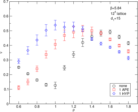
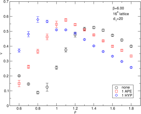
Figure 11: Localization $\nu$ vs. $\rho$ at $\beta\!=\!5.84$ (left) and $\beta\!=\!6.00$ (right) with no filtering, 1 APE or 1 HYP step. This is the only case where we deviate from our convention to define $\nu$ via (29) and use $d_{1}\!=\!{5\over 4}L$.

There is a loose connection between the localization of $D_{\mathrm{ov}}$ and the spectrum of $H_{\mathrm{W}}$, for instance

$$||D_{\mathrm{ov}}(x,y)||\leq\mathrm{const}\times\exp(-{\theta\over 2}||x-y||_{1})$$ (10)

is a bound found in [30], where $||.||$ is the matrix norm in Dirac and color space. The exponent $\theta/2$ in (10) is defined via the largest and smallest eigenvalue of $D_{\mathrm{W},-\rho}^{\dagger}D_{\mathrm{W},-\rho}$ through

$$\cosh(\theta)={\lambda_{\mathrm{max}}/\lambda_{\mathrm{min}}+1\over\lambda_{\mathrm{max}}/\lambda_{\mathrm{min}}-1}={1+\epsilon^{2}\over 1-\epsilon^{2}}$$ (11)

where we like to express the r.h.s. in terms of the inverse condition number $\epsilon$ of $|H_{\mathrm{W}}|$. Expanding either side to first order one obtains the simple relation (after getting rid of the unphysical $\theta\!<\!0$ solution)

$${\theta\over 2}=\epsilon+O(\epsilon^{2})\;.$$ (12)

As already mentioned in [30] the exponent $\theta/2$, defined via the spectral properties of the underlying $|H_{\mathrm{W}}|$, is a rather bad estimate for the actual localization $\nu$. The situation is not much better for the filtered variety, as a brief comparison of our Tabs. 3 and 4 reveals. Though quantitatively unsuccessful, this connection still gives a qualitative hint that the overlap operator with a filtered Wilson kernel might enjoy better localization properties due to the reduced condition number of $H_{W}$. There are more detailed bounds in the literature [32, 33, 34, 35, 36], but it seems fair to say that a quantitative understanding of the localization of $D_{\mathrm{ov}}$ in terms of the spectral properties of $H_{W}$ is a challenge.

The localization $\nu$ as a function of the projection parameter $\rho$ is presented in Fig. 11. For $\beta\!=\!5.84,6.00$ the optimum parameter for the unfiltered operator is around $\rho\!=\!1.6,1.4$, respectively. For the 1 HYP operator the localization at $\rho\!=\!1.0$ does not fall short of the maximal one by a large amount; this is why we restrict much of our investigation with a filtered $D_{\mathrm{ov}}$ to the case $\rho\!=\!1.0$. Still, the figure suggests that an optimal $\rho$ for the 1 HYP filtered operator may be smaller than 1, and it decreases with increasing $\beta$; at $\beta\!=\!5.84$ we find $\rho_{\mathrm{opt}}^{\mathrm{1\,HYP}}\!\simeq\!1.0$ and at $\beta\!=\!6.00$ we find $\rho_{\mathrm{opt}}^{\mathrm{1\,HYP}}\!\simeq\!0.8$.

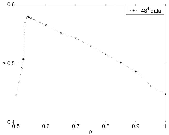
Figure 12: Localization (29) in the free field case with an extremum at $\rho_{\mathrm{opt}}^{\mathrm{free}}\!\simeq\!0.54$ and a steep descent to the left. Note that in the $\rho$ range shown the inverse condition number $\epsilon\!=\!\rho/(8\!-\!\rho)$ is monotonic.

After dealing with some technical issues to make sure that an $48^{4}$ lattice is large enough (see App. B), we have studied $\nu$ defined via (29) as function of $\rho$ in the free case; the result is shown in Fig. 12. The pattern observed in Fig. 11 should thus not come as a surprise, filtering simply drives the locality properties of the overlap operator towards the free field case. In fact, Fig. 12 offers a simple explanation why it is so difficult to predict the localization $\nu$ from spectral properties of the underlying $|H_{\mathrm{W}}|$ operator – in the free case the inverse condition number (6) in the range $0\!<\!\rho\!<\!1$ is monotonic, while $\nu$ has a non-trivial extremum at $\rho_{\mathrm{opt}}^{\mathrm{free}}\!\simeq\!0.54$.

4 Kernel non-normality

An operator $A$ is called normal, if it commutes with its adjoint

$$[A,A^{\dagger}]=0$$ (13)

which implies that its left and right eigenbasis coincide. Normality has special implications for lattice Dirac operators. For a normal Dirac operator $D=\sum_{k}\lambda_{k}|k\rangle\langle k|$ which, in addition, is $\gamma_{5}$-hermitean

$$\gamma_{5}D\gamma_{5}=D^{\dagger}$$ (14)

we immediately obtain

$$D^{\dagger}=\sum_{k}\lambda_{k}^{*}|k\rangle\langle k|=\sum_{k}\lambda_{k}\gamma_{5}|k\rangle\langle k|\gamma_{5}$$ (15)

and this implies that eigenmodes with real $\lambda_{k}$ are chiral (or may be linearly combined to chiral modes in case of degeneracies). Furthermore, for such a $D$ the eigenvectors of the hermitean Dirac operator

$$H=\gamma_{5}D=\sum_{k}\lambda_{k}\gamma_{5}|k\rangle\langle k|$$ (16)

are given by $\sqrt{\lambda_{k}^{*}}|k\rangle\pm\sqrt{\lambda_{k}}\gamma_{5}|k\rangle$ with the corresponding eigenvalues $\pm|\lambda_{k}|$.

The continuum Dirac operator is normal, and so are the naive and staggered discretizations (but the latter two yield more than one flavor in the continuum limit). The GW relation (1) together with $\gamma_{5}$-hermiticity (14) also implies normality of the operator, hence $D_{\mathrm{ov}}$ is normal. In fact, the overlap construction can be described as extracting the unique unitary part of $D_{\mathrm{kern}}/\rho$ [37], and for a normal kernel it reduces to a simple radial projection of the $D_{\mathrm{kern}}/\rho$ eigenvalues onto the unit circle.

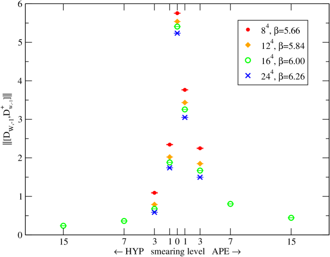
Figure 13: Non-normality (in lattice units) of the Wilson kernel, as defined in (17), as a function of smearing. The improvement of the kernel normality does not seem to degrade towards the continuum.

The shifted Wilson operator, which we use as a kernel, is not normal. Some consequences of this non-normality have been explored in other contexts [38]. Here, it suffices to point out that the relations between the eigenmodes of the overlap operator, its kernel and the hermitean Dirac operator are not as simple as above for the case of a normal operator. Typically, an eigenvector of the (hermitean) kernel will mix into every mode of the overlap operator, which we expect to have a detrimental effect on the efficiency of overlap construction algorithms. Thus, a practically relevant question is whether UV filtering can reduce the amount of non-normality of the overlap kernel.

To quantify the non-normality of $D_{\mathrm{W}}$ we measure the 2-norm of the commutator; technically

$$||[D_{\mathrm{W},-1},D_{\mathrm{W},-1}^{\dagger}]|\eta\rangle||$$ (17)

is averaged over a number of normalized random vectors $|\eta\rangle$. In Fig. 13 the commutator (17) is shown for all $\beta$ and smearing levels (since this is not a physical observable, we use lattice units). Evidently, any kind of filtering reduces it – the filtered kernel is thus closer to normality and has left- and right-eigenvectors that are better aligned than for the unfiltered version. Whether “smart” overlap construction algorithms can be written which exploit this property is an open question.

5 Physics perspectives

To explore the physics potential of filtered overlap quarks a quenched spectroscopy study would be highly desirable. Physical results should reproduce – after a continuum extrapolation – results in the traditional “thin link” formulation. It would be interesting to see whether the speedup in point 1 of the introduction gets enhanced in points 2-4; in particular if scaling and/or asymptotic scaling set in earlier, this would make a real difference. Unfortunately, a detailed scaling study requires substantial computational resources, but as a first step in this direction we want to investigate the renormalization of the axial-vector current with filtered overlap quarks.

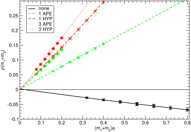
Figure 14: $m_{1}^{\mathrm{AWI}}\!+\!m_{2}^{\mathrm{AWI}}$ vs. $m_{1}^{\mathrm{bare}}\!+\!m_{2}^{\mathrm{bare}}$ [$\mathrm{slope}\!=\!Z_{A}^{-1}$] at $\beta\!=\!5.66$ . Without filtering $Z_{A}\!<\!0$, while any filtering prescription gives $Z_{A}\!>\!1$, with higher filtering levels resulting in a value closer to 1.

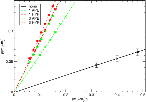
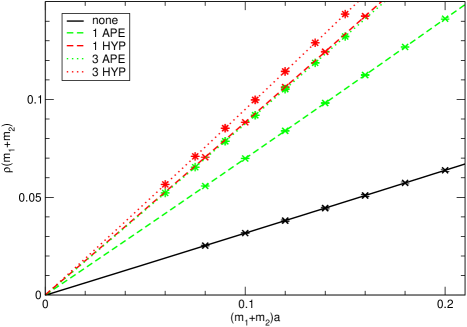
Figure 15: $m_{1}^{\mathrm{AWI}}\!+\!m_{2}^{\mathrm{AWI}}$ vs. $m_{1}^{\mathrm{bare}}\!+\!m_{2}^{\mathrm{bare}}$ at $\beta\!=\!5.84,6.00$. Higher filtering levels shift $Z_{A}$ closer to 1.

We follow the method of [39, 40, 41], where one starts from the usual (chirally rotated) densities

$$P(x) = \psi_{1}(x)\gamma_{5}[(1-{1\over 2\rho}D_{\mathrm{ov}})\psi_{2}](x)$$ (18)

$$A_{\mu}(x) = \psi_{1}(x)\gamma_{\mu}\gamma_{5}[(1-{1\over 2\rho}D_{\mathrm{ov}})\psi_{2}](x)$$ (19)

with $\psi_{1}\!\neq\!\psi_{2}$ (flavor non-singlet) and defines the correlators [$x\!=\!(\mathbf{x},t)$]

$$G_{PP}(t) = \sum_{\mathbf{x}}P(\mathbf{x},t)P^{c}(\mathbf{0},0)$$ (20)

$$G_{\nabla\!AP}(t) = \sum_{\mathbf{x}}\bar{\nabla}_{\!4}\!A_{4}(\mathbf{x},t)P^{c}(\mathbf{0},0)$$ (21)

where $\bar{\nabla}_{\!4}$ is the symmetric derivative in the time direction and $P^{c}$ is the conjugate of (18), i.e. with the flavor indices $1\!\leftrightarrow\!2$ interchanged. With these correlators at hand one forms the ratio

$$\rho(t,m_{1},m_{2})={G_{\bar{\nabla}\!AP}(t)\over G_{PP}(t)}$$ (22)

where the second and third argument indicate that the spinors $\psi_{1}$ and $\psi_{2}$ in the densities (18, 19) are solutions to the massive operators $D_{\mathrm{ov},m_{1}}$ and $D_{\mathrm{ov},m_{2}}$, respectively. On account of the axial Ward identity (AWI) the ratio $\rho$ should be constant in time, and for light enough quarks (22) tends indeed to plateau rather nicely (see e.g. Fig. 1 in [41]). In a slightly sloppy but transparent notation the plateau value is $\rho(m_{1},m_{2})$. This quantity will – to the extent to which the AWI is respected at finite lattice spacing – only depend on the sum of the quark masses, and thus defines the $m^{\mathrm{AWI}}$ quark masses

$$\rho(m_{1},m_{2})=\rho(m_{1}\!+\!m_{2})\;+\;O(a^{2})=m_{1}^{\mathrm{AWI}}+m_{2}^{\mathrm{AWI}}\;+\;O(a^{2})\;.$$ (23)

The actual data for our $Z_{A}$ determination for quenched filtered and unfiltered overlap quarks are generated with couplings and geometries as given in the last line of Tab. 1. We restrict ourselves to the canonical choice $\rho\!=\!1$. We plot $\rho(m_{1},m_{2})$ versus $m_{1}\!+\!m_{2}$ for various quark mass combinations and filtering levels in Fig. 14 for $\beta\!=\!5.66$ and in Fig. 15 for $\beta\!=\!5.84,6.00$, respectively. They form one universal band, i.e. different $m_{1}$ and $m_{2}$ combinations with a fixed sum $m_{1}\!+\!m_{2}$ always give the same $\rho(m_{1}\!+\!m_{2})$ [within errors]. Furthermore, the relationship is in good approximation linear, but there is an anomaly without filtering at our strongest coupling (Fig. 14). Here, the slope is negative, and this supports the view established in App. A that with $\beta\!=\!5.66$ and $\rho\!=\!1.0$ the projection point is “in” or “to the left” of the physical branch of the underlying Wilson operator, and we effectively operate in the “zero fermion” sector. Also at $\beta\!=\!5.84$ the unfiltered plateau was not very pronounced either, resulting in a large systematic uncertainty beyond the statistical error quoted below. We use the ansatz

$$\rho(m_{1}\!+\!m_{2})=\mathrm{const}+{1\over Z_{A}}(m_{1}\!+\!m_{2})+\mathrm{const}\,(m_{1}\!+\!m_{2})^{2}$$ (24)

and see whether we obtain acceptable fits and whether the first constant is consistent with zero. It turns out that this is the case, and the associate $Z_{A}$ values are summarized in Tab. 5.

$\beta$	$5.66$	$5.84$	$6.00$	$6.00\;(\rho=1.4)$
$Z_{A}^{\mathrm{none}}$	ill-def.	7.06(73)	3.145(94)	1.554(1)[41]
$Z_{A}^{\mathrm{1\,APE}}$	2.57(7)	1.66(02)	1.452(04)	—
$Z_{A}^{\mathrm{3\,APE}}$	1.55(3)	1.23(01)	1.160(06)	—
$Z_{A}^{\mathrm{1\,HYP}}$	1.44(2)	1.22(01)	1.153(03)	—
$Z_{A}^{\mathrm{3\,HYP}}$	1.21(1)	1.10(01)	1.072(02)	—
$Z_{A}^{\mathrm{none}}|_{\mathrm{1-loop}}$ [43]	1.280	1.272	1.264	1.120

Table 5: $Z_{A}$ determined via (24) with various filtering prescriptions. On the last line the 1-loop result [43] for the thin-link overlap $Z_{V,A}=1+C_{F}\,0.198206g_{0}^{2}+O(g_{0}^{4})=1+1.585648/\beta+O(1/\beta^{2})$ at $\rho\!=\!1.0$ and $Z_{V,A}=1+C_{F}\,0.090301g_{0}^{2}+O(g_{0}^{4})=1+0.722408/\beta+O(1/\beta^{2})$ at $\rho\!=\!1.4$ is added for comparison.

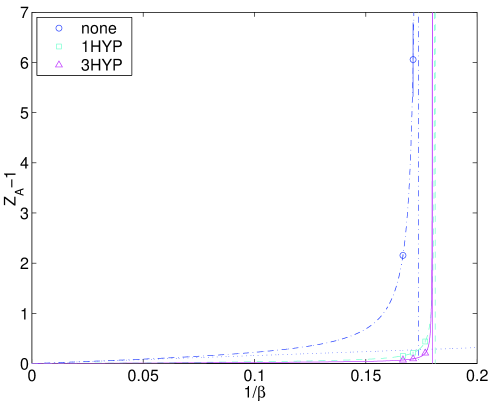
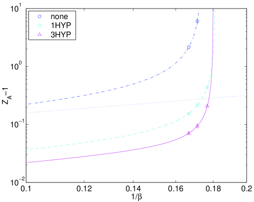
Figure 16: Pade functional forms through our $\rho\!=\!1$ data in standard (left) or double logarithmic form (right). In the unfiltered case the constraint to reproduce the known 1-loop behavior is built in and the latter is indicated with a dotted line. It seems the 1-loop coefficients of the filtered $Z_{A}$ are dramatically reduced, while the perturbative range (blow-up point of the Pade ansatz) gets barely enlarged.

It is interesting to discuss both the general pattern of these $Z_{A}$ values and the relation to 1-loop perturbation theory. Evidently, at fixed $\beta$ and $\rho$ the filtered $Z_{A}$ is much closer to the tree-level value 1. We recover the relative strength ordering of Sect. 2, i.e. one APE step is less efficient than 3 APE or a single HYP step, but the latter is topped by 3 HYP steps. At $\beta\!=\!6.0$ we compare to $\rho\!=\!1.4$ which is the the standard choice for the “thin link” overlap. Without filtering, $Z_{A}^{\mathrm{none}}(\rho\!=\!1.4)\!\simeq\!1.554$ is about half of $Z_{A}^{\mathrm{none}}(\rho\!=\!1.0)\!\simeq\!3.145$, and this means that the choice $\rho\!=\!1.4$ is not just near-optimal w.r.t. locality, but also beneficial to tame (one particular) renormalization. Once the filtering recipe is specified, $Z_{A}$ seems to be monotonic in $6/\beta\!=\!g_{0}^{2}$, as expected from perturbation theory. In the unfiltered case the 1-loop value is included in the last line of Tab. 5 for comparison. Assuming that in perturbation theory $1\!<\!Z_{A}^{\mathrm{1\,HYP}}\!<\!Z_{A}^{\mathrm{none}}$ holds for $\rho\!=\!1$, one may compare the deviation of the unfiltered $\beta\!=\!6.0$ operator $3.145\!-\!1.264\!=\!1.881$ to $1.153\!-\!1\!=\!0.153$ which then amounts to an upper bound in the 1 HYP case. Evidently, the discrepancy is dramatically reduced, which in view of the perturbative results in [44, 45], should not come as a surprise. To get a slightly more quantitative view, we consider it useful to fit our data without filtering at $\rho\!=\!1$ to a Pade-type ansatz of the form

$$Z_{A}^{\mathrm{none}}={1+c_{1}x+c_{2}x^{2}\over 1+(c_{1}-1.585648)x}$$ (25)

with $x\!=\!1/\beta$, where the perturbative knowledge [43] (cf. caption of Tab. 5) is built-in as a constraint. In the same spirit a Pade ansatz for any of the filtered operators reads

$$Z_{A}^{\mathrm{1HYP\,/\,3HYP}}={1+c_{1}x+c_{2}x^{2}\over 1+c_{3}x}$$ (26)

with – as of now – no constraint on $c_{1}\!-\!c_{3}$ yet. There is a problem with the functional forms (25, 26), since our data sets contain 2 and 3 entries, respectively, and there is zero degree of freedom. Still, for an illustration such a “fit” might be worth while, and the result is shown in Fig. 16. With sufficient data the curves would contain two pieces of information. The asymptotic slope for $x\!\to\!0$ would predict the perturbative 1-loop coefficients for $Z_{A}^{\mathrm{1\,HYP}}$, $Z_{A}^{\mathrm{3\,HYP}}$. And the pole in (25, 26), i.e. the values $c_{1}-1.585648$ or $c_{3}$, respectively, would predict the coupling where the perturbative description breaks down. Hence, if the curves in Fig. 16 are indicative at all, it seems that filtering renders the perturbative 1-loop coefficient of $Z_{A}$ much smaller, but the perturbative range gets barely enhanced.

6 Discussion

In this paper we have studied the massless overlap operator constructed from a filtered Wilson kernel where the original “thin” links were replaced by “thick” links which behave in the same manner under local gauge transformations. This is a legal change of the fermion discretization as long as one particular filtering recipe [e.g. 1 HYP step with $\alpha_{\mathrm{HYP}}\!=\!(0.75,0.6,0.3)$] is maintained at all couplings. It amounts to an $O(a^{2})$ re-definition of $D_{\mathrm{ov}}$ at fixed $\rho$, as does a change of $\rho$ at fixed filtering level.

Our key observations are the following. First, the onset of the “bulk” part of the spectrum of the underlying shifted hermitean Wilson operator $H_{\mathrm{W}}\!=\!\gamma_{5}(D_{\mathrm{W}}\!-\!\rho)$ gets lifted. This leads to an increased inverse condition number $\epsilon$ (after projection typically by a factor 2-4 through a single HYP step) and the latter reflects itself in a reduction (by the same factor) of the polynomial degree (and thus the number of forward applications of $H_{\mathrm{W}}^{2}$) needed to construct the inverse square root over the relevant range. What is the precise impact on CPU requirements to invert the massive operator is a topic for future research. Second, at standard couplings the filtered massless overlap is – even with the untuned canonical choice $\rho\!=\!1$ – better localized than the unfiltered version with an optimally tuned $\rho$ could ever be. Our finding is backed by the observation that in the free case the optimum $\rho$ (w.r.t. locality) is around $0.54$ and thus substantially smaller than the typical $\rho\!\simeq\!1.4$ used in the past. Our third observation is that the filtered kernel is much closer to being a normal operator. In other words the left- and right-eigenvectors of $D_{\mathrm{W}}$ are better aligned with higher filtering level, and in this respect the effect of the “thick” links is the same as a shift much closer towards the continuum under which the overlap construction (3) tends to be a simple radial projection of the $D_{\mathrm{W}}$ eigenvalues. Finally, our fourth observation is that the renormalization constant of the axial-vector current is much closer to 1 with filtering than without. We rate this as a sign that lattice perturbation theory for the filtered overlap might work much better than for the unfiltered variety. If this is indeed so, and if it goes through for 4-fermion operators, it is likely to be the most important consequence of our work, since it offers the perspective of considerably reduced theoretical uncertainties in electroweak precision studies.

Let us finally discuss a variety of proposals in the literature that are similar in spirit to the one put forth in the present paper.

There is a top-level version deriving from “parametrized fixed-point fermions”. The idea behind this approach pursued by Hasenfratz and Niedermayer is that true fixed-point fermions would satisfy the GW relation exactly [8], but a practical implementation is always ultralocal. Hence, sticking such an ansatz into the overlap formula (3) yields fermions with exact chiral symmetry and otherwise properties that are at least as good (but typically better) than the version with a plain Wilson kernel [46].

Bietenholz has considered a variety of actions, originally based on RG concepts [47]. The idea was that an action with a spectrum close to the GW circle could be iteratively improved in its chiral properties. Over time the focus has shifted towards using the overlap formula (3) to have exact chiral symmetry, but it is clear that the kernel of his “hypercubic overlap” benefits from a larger inverse condition number $\epsilon$ of $|\gamma_{5}D_{\mathrm{kern}}|$ just as we do.

Gattringer and collaborators construct a “chirally improved” Dirac operator that involves the full Dirac Clifford algebra with links restricted to the hypercube. The coefficients are adjusted such that (for a given coupling) the violation of the GW relation is minimized [48]. The problem is the same as in the Bietenholz approach: a single forward application with such a kernel is so expensive that the improvement, if it is not “perfect”, does not really pay off.

DeGrand has considered – both perturbatively and non-perturbatively – Wilson and clover action varieties that involve smeared gauge links [49, 44]. Based on this experience he went on to construct a “variant overlap” which starts from a kernel with only scalar/vector terms and smoothed links, and is thus sufficiently cheap as to allow for sticking it into the overlap formula [50, 45].

The closest to what we do is found in the work of Kovacs [31]. He uses a “fat-link clover” overlap in which all links are smeared, together with the tree-level value $c_{\mathrm{SW}}\!=\!1$. As far as we know, he was the first author to notice that such a filtered kernel allows for the untuned choice $\rho\!=\!1$, and still the resulting overlap shows good localization properties.

A related approach has been pursued by the Adelaide group [51]. Their “fat link irrelevant clover” overlap quarks are built from a clover action in which only the irrelevant pieces (i.e. the Wilson and the Sheikoleslami-Wohlert terms) use smeared links, but not the covariant derivative. They found a similar speedup factor in the construction of the overlap operator (cf. “step 1” in the introduction) and tied it to the reduced spectral density of $|\gamma_{5}D_{\mathrm{kern}}|$ near the origin.

Finally, “overlap” quarks with smeared gauge links have been used by several lattice collaborations. RBC has found that the residual mass of domain-wall fermions at fixed $N_{5}$ gets reduced [52], though they miss out an important ingredient, the projection to $SU(3)$. UKQCD has used overlap valence quarks with 3-fold HYP smeared links on staggered sea as supplied by the MILC collaboration, finding a surprisingly good signal on as few as 10 configurations [53]. Similarly, LHP and NPLQCD have used filtered domain-wall valence quarks on staggered sea to compute the pion form factor [54] and the $I\!=\!2$ $\pi\pi$-scattering length [55], respectively.

There is another idea that should not be confused with filtering. Using an improved gauge action has been found to reduce $\rho_{|H_{\mathrm{W}}|}(0)$ by up to an order of magnitude [56, 57, 58]. There is, however, an important practical difference to the filtering concept, which is a modification of the fermion action. As already discussed in [13], a better choice of the gauge action improves, in the first place, the very low end of the $|H_{\mathrm{W}}|$ eigenvalue distribution. After projecting out the lowest $O(15)$ eigenvectors (which nowadays is a standard thing to do [18]) much of the advantage is lost (in Fig. 3 of [58] the lifting factor diminishes to the right). By contrast, filtering lifts the complete low-energy end of the $|H_{\mathrm{W}}|$ eigenvalues (in our Fig. 3 one finds an almost-universal lifting factor) and the usefulness of filtering is not vitiated by the projection. Still, it might be interesting to see whether the two ideas can be fruitfully combined.

An extension of the filtering concept to full QCD is straightforward, albeit hampered by a technical problem. These days, most dynamical fermion simulations are set up with a HMC algorithm, and the latter requires the fermion action to be differentiable w.r.t. the gauge links. The kernel of our filtered overlap quarks is differentiable w.r.t. the “thick” links, but not w.r.t the elements of the original set, due to the projection involved in the APE [10] or HYP [11] procedure. A convenient way out is offered by the stout/EXP links introduced in [59], involving a differentiable mapping between the “thick” and “thin” links. In pure gauge observables the usefulness of this smearing recipe was found to be restricted to small parameter values [59, 20], and one may fear that this feature persists in stout/EXP overlap quarks, since in perturbation theory they are equivalent to APE filtered overlap fermions with $\alpha_{\mathrm{APE}}=1/(1-6\alpha_{\mathrm{EXP}})$ [60]. Thus, due to the pole at $\alpha_{\mathrm{EXP}}\!=\!1/6$ we expect them to have a “narrow therapeutic range” in parameter space, but it is clear that there is no conceptual issue in simulating full QCD with filtered overlap quarks beyond the difficulties met in the unfiltered case [61].

To summarize, our suggestion is to use the overlap recipe (3) with an unimproved ($c_{\mathrm{SW}}\!=\!0$) Wilson kernel in which all links are replaced by some smeared descendents of the actual gauge background. We recommend to stay with a moderate amount of link “fattening”, e.g. with a single step of standard HYP smearing [11]. The projection parameter $\rho$ may be fixed at its canonical value 1, and in this sense the filtered overlap involves less tuning than the unfiltered version. An important restriction is that the choice of iteration level and smearing parameter must be the same for all couplings considered in a scaling study. This is one point on which our proposal differs from some of the attempts reviewed above which involve coefficients (e.g. in the extended $\gamma$-algebra) that are adjusted “by hand” to yield a GW-type spectrum at one standard value of the gauge coupling. The other difference is that our kernel remains cheap and still requires fewer $D_{\mathrm{kern}}^{\dagger}D_{\mathrm{kern}}$ forward applications. From a practical viewpoint, a clear advantage is the ease of implementation of the “filtered overlap” — everyone with a running overlap code has it (in disguise).

Acknowledgments

It is a pleasure to thank Ferenc Niedermayer and Tom DeGrand for useful conversation or correspondence. This paper was supported by the Swiss NSF.

App. A: Cumulative eigenvalue distributions in 4D and 2D

In this appendix we discuss what can be learned from the cumulative eigenvalue distribution (CED). We consider both the eigenvalues in 4D generated for the main part of this paper and data from dedicated runs in the quenched Schwinger model (QED with massless fermions in 2D) to elucidate the effects that filtering and changing $\beta$ have on the spectral density of the hermitean Wilson operator $H_{\mathrm{W}}\!=\!\gamma_{5}D_{\mathrm{W},-1}$.

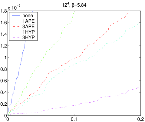
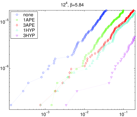
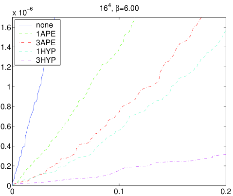
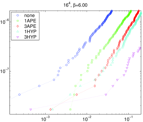
Figure 17: Cumulative eigenvalue distribution (CED) of $|H_{\mathrm{W}}|$ in standard (left) or double logarithmic (right) form for $\beta\!=\!5.66,5.84,6.00$ (from top to bottom) with 0,1,3 steps of APE or HYP filtering. At each $\beta$ the upper cut in the vertical direction is the same on the left and on the right and the upper end in the horizontal direction is 0.2 throughout. Note the change in the ordinate scale between different couplings. At $\beta\!=\!6.26$ we definitely lack the statistics needed to see a linearly dominated regime.

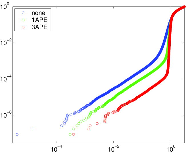
Figure 18: Log-log plot of the cumulative eigenvalue distribution (CED) of $|H_{\mathrm{W}}|$ in the Schwinger model (${N_{\!f}}\!=\!0$, $16^{2}$ geometry, $\beta\!=\!3.2$, $\rho\!=\!1$) without filtering (top curve) and after 1 or 3 filtering steps. In all cases the CED starts out linearly, raises sharply somewhere near $\lambda\!\simeq\!1$ and reaches 1 at $\lambda\!\simeq\!3$ (in 2D). This figure includes all eigenvalues of all three operators on 22,500 decorrelated configurations.

Fig. 17 presents the cumulative eigenvalue distribution (CED) of the 15 smallest eigenvalues of $|H_{\mathrm{W}}|$ on the ensembles discussed before. We show it both in standard form and in double logarithmic form, and the scale on the ordinate follows from the requirement that it would extend up to 1, if all eigenvalues were calculated (cf. Fig. 18 below). For the two intermediate couplings ($\beta\!=\!5.84,6.00$) we see the expected linear rise of the CED near the origin, which soon gets complemented by a higher order piece. The coefficient of the linear part is a measure for the spectral density of the hermitean Wilson operator at the origin, $\rho_{|H_{\mathrm{W}}|}(0)$. That density being non-zero means that there is a finite probability to encounter arbitrarily small eigenvalues. The main effect of smearing is to reduce this spectral density, as is evident from the double logarithmic plots – here the initial slope 1 piece gets shifted downwards, and this corresponds to a smaller coefficient in front of the linear piece in the standard representation. Our data at $\beta\!=\!6.26$ are of lesser quality – here we definitely cannot identify a linearly dominated regime. The situation is far more favorable in Fig. 18 where quenched Schwinger model data are shown. Apart from the statistics, the main difference is that all eigenvalues (extending up to $\,\sim\!3$ in 2D) are included. The higher the filtering level or $\beta$, the more pronounced is the “jump” in the CED at $\lambda\!\simeq\!1$. Note that with a chiral kernel all eigenvalues of $|\gamma_{5}D_{\mathrm{kern}}|$ would be there, i.e. the CED would be a step function at $\lambda\!=\!1$. Finally, to come back to Fig. 17, the situation at the strongest coupling ($\beta\!=\!5.66$) is different, since here the linear piece in the unfiltered CED is not larger than in the filtered versions. This is, because our choice $\rho\!=\!1$ lets us “loose” the fermion – at this coupling our projection point is somewhere “in” the physical branch or “to the left” of it, while for the filtered version $\rho\!=\!1$ is still appropriate. One might avoid such a situation by choosing a larger $\rho$ with the unfiltered kernel, but an even safer option might be to refrain from simulating unfiltered overlap quarks on such coarse lattices. It looks like this is a situation where the filtered overlap may help a lot, since it allows simulations on coarser lattices than the unfiltered operator, but in order to really be useful such simulations should be in the scaling regime (and not just in the right universality class), and this is, of course, not yet clear.

The spectral properties of $H_{\mathrm{W}}$ play a role in the context of the physical interpretation of the Aoki phase [62]. The latter is a conjectured phase, originally specific to ${N_{\!f}}\!=\!2$ active Wilson fermions at negative mass, in which after switching off an external trigger term

$$S_{\mathrm{source}}=\pm h\overline{\psi}\gamma_{5}\sigma_{3}\psi$$ (27)

parity and flavor break spontaneously and a condensate ($\mathrm{const}\neq\!0$)

$$\lim_{h\to 0^{\pm}}\langle\overline{\psi}\gamma_{5}\sigma_{3}\psi\rangle=\pm\mathrm{const}$$ (28)

forms. Good numerical evidence for a non-zero condensate (28) in the (dynamical) 2-flavor case for an appropriate choice of the negative mass $-\rho(\beta)$ is found in [63]. Ref. [64] argues that in the massless limit of the continuum theory a condensate of the form (28) is simply an axial rotation of the usual (flavor diagonal) condensate and thus breaks neither parity nor flavor. They relate the spectral density of $D_{\mathrm{W}}$ to that of $H_{\mathrm{W}}$ and argue that the absence of a gap (around the origin) of the latter is indicative of chiral symmetry breaking and that $\rho_{|H_{\mathrm{W}}|}(0)\!>\!0$ if and only if (28) is non-zero. This was later elucidated to be a continuum argument [65], which – in view of our Sec. 4 – might be an important point.

The next issue is whether there is an Aoki phase in the quenched theory with 2 valence (but 0 sea) flavors [66, 67]. The simplest expectation is that qualitatively the picture with the 5 Aoki “fingers” goes through, though the phase boundary is somewhat shifted w.r.t. the ${N_{\!f}}\!=\!2$ case.

Our 4D data in Fig. 17 clearly show the suppression of $\rho_{|H_{\mathrm{W}}|}(0)$ as one approaches the continuum, but we cannot see any sign that this distribution would vanish at some “critical” coupling. Given the uniform pattern in the figures (apart from the scale on the $y$-axis they seem qualitatively similar), it seems more likely to us that $\rho_{|H_{\mathrm{W}}|}(0)$ will stay non-zero for arbitrary couplings.

To test this view, we analyze the quenched Schwinger model where high statistics can be reached. The couplings and geometries are chosen such as to have a fixed physical volume, with a box size about 5 times larger than the Compton wavelength of the lightest degree of freedom in the chiral limit of the ${N_{\!f}}\!=\!1$ theory. A survey of the parameters is given in Tab. 6 and for technical details we refer to [14].

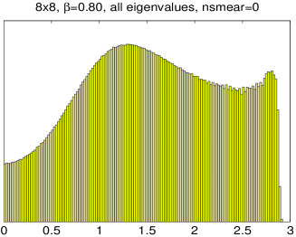
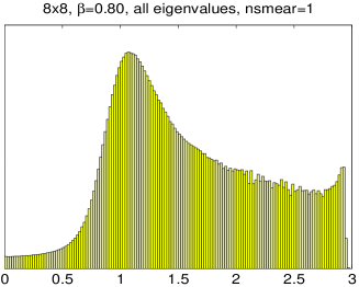
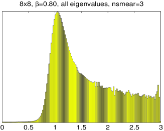
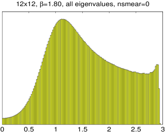
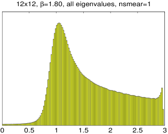
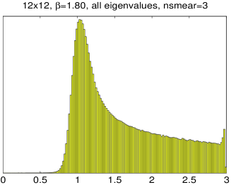
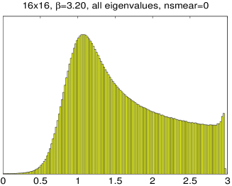
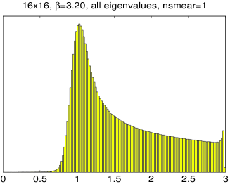
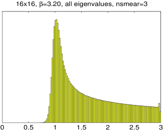
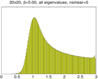
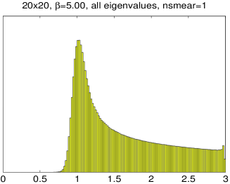
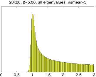
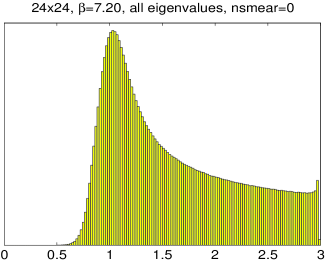
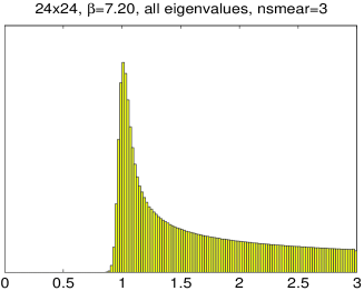
Figure 19: Distribution of all eigenvalues of $|H_{\mathrm{W}}|\!=\!|\gamma_{5}D_{\mathrm{W},-1}|$ at five $\beta$ and 0,1,3 smearings.

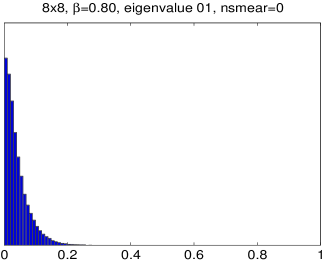
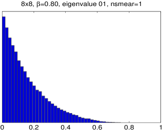
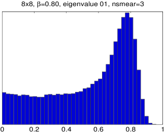
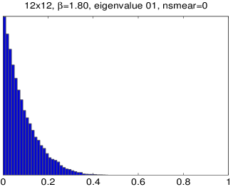
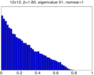
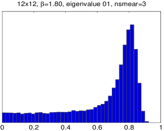
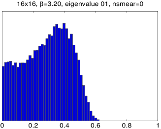
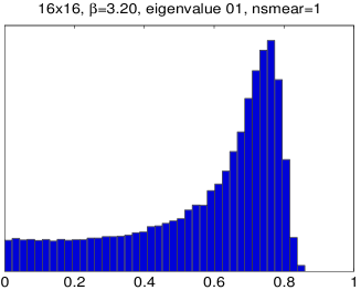
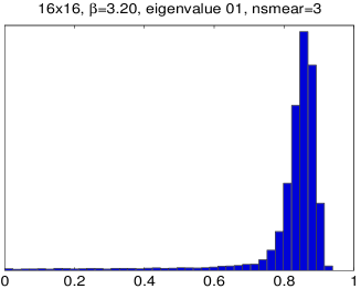
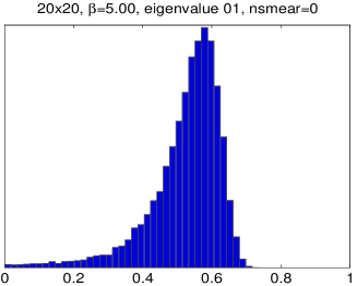
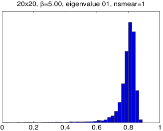
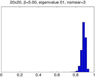
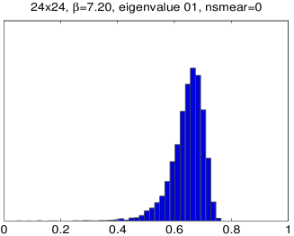
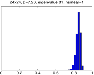
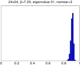
Figure 20: Distribution of the 1st eigenvalue of $|H_{\mathrm{W}}|\!=\!|\gamma_{5}D_{\mathrm{W},-1}|$ at five $\beta$, with 0,1,3 smearings.

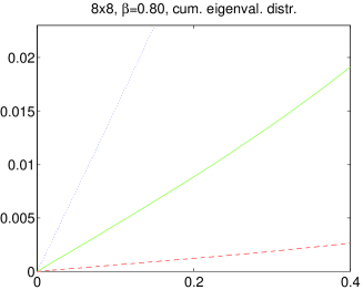
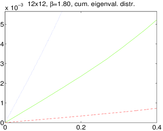
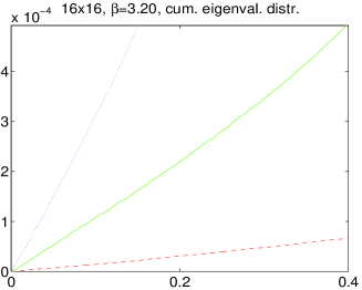
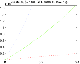
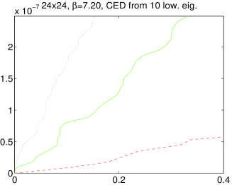
Figure 21: Cumulative eigenvalue distribution of $|H_{\mathrm{W}}|\!=\!|\gamma_{5}D_{\mathrm{W},-1}|$ at five $\beta$, with 0,1,3 smearings.

Fig. 19 provides an overview over the complete $|H_{\mathrm{W}}|$ eigenvalue distribution; one sees a “peak” at $\lambda\!=\!1$ forming that gets more pronounced with higher $\beta$ and higher filtering level. This “peak” corresponds to the “jump” at $\lambda\!=\!1$ in the CED of $|H_{\mathrm{W}}|$ in Fig. 18.

Fig. 20 presents the distribution of the lowest eigenvalue of $|H_{\mathrm{W}}|$. At low $\beta$ this distribution accumulates at zero, at intermediate values of the coupling there is a horizontal band of eigenvalues connecting down to zero, and at the largest $\beta$ there are just scattered eigenvalues. Evidently, one cannot draw a final conclusion whether these scattered eigenvalues really make up for a non-zero $\rho(0)$, but it seems worth while to study this band in the region of $\beta$ values where it is clearly visible and see whether changing $\beta$ implies some structure, or whether it just stays flat, regardless of $\beta$.

Fig. 21 presents the CED in the area of interest, the very-low $\lambda$ region. At $\beta\!=\!5.0,7.2$ we show the data from the high-statistics run with 10 eigenvalues per configuration (bottom line of Tab. 6), but we checked that the results are consistent with what we get from the runs where all eigenvalues were determined. At a given coupling filtering clearly reduces $\rho_{|H_{\mathrm{W}}|}(0)$. The overall impression is that changing $\beta$ merely rescales the $y$-axis, in striking analogy with what we have seen in 4D (Fig. 17). If this is indeed true, the natural conclusion is that $\rho_{|H_{\mathrm{W}}|}(0)\!>\!0$ at any finite $\beta$ in the quenched theory.

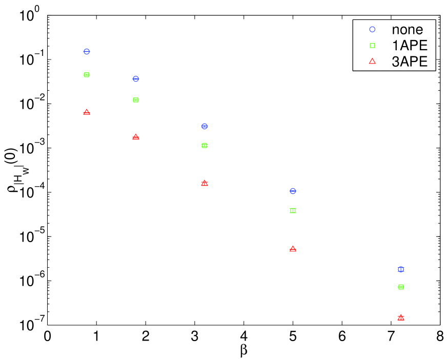
Figure 22: $\rho_{|H_{\mathrm{W}}|}(0)$ versus $\beta$ in the quenched Schwinger model. Filtering seems to reduce, for all $\beta$, the eigenvalue density by a near-universal factor. The data suggest an exponential fall-off at large $\beta$.

Fig. 22 contains a summary of our determinations of the spectral densities $\rho_{|H_{\mathrm{W}}|}(0)$ for various $\beta$ and filtering levels, extracted from the initial slopes in the CED shown in Fig. 21. It looks like eventually the density decreases exponentially in $\beta$ and changing the filtering level amounts to an overall rescaling factor which is, in good approximation, independent of $\beta$. Obviously, this is just numerical evidence, but the message seems to be as clear as one can possibly hope for from a numerical experiment. Note that for practical reasons we cannot take the infinite volume limit, but given our physical box size we expect finite volume effects to be exponentially small.

$\beta$	$0.8$	$1.8$	$3.2$	$5.0$	$7.2$
geometry	$8\!\times\!8$	$12\!\times\!12$	$16\!\times\!16$	$20\!\times\!20$	$24\!\times\!24$
statistics	90,000	40,000	22,500	14,400	10,000
statistics	—	—	—	275,000	75,000

Table 6: Matched quenched 2D lattices; reweighting to ${N_{\!f}}\!=\!1$ the lightest particle in the chiral limit would fit $5$ times into the box. In the first set all $|H_{\mathrm{W}}|$ eigenvalues are determined with statistics such as to have an equal number of eigenvalues. In the second set only the lowest 10 eigenvalues are computed.

We remind the reader that (both in 2D and in 4D) we were working at fixed negative mass $m_{0}\!=\!-1$ and pushed towards the continuum line. In other words, we were trying to stay as far outside the Aoki phase as one can, if one wants to be in the supercritical region with one overlap fermion. Of course, our data do not exclude the existence of a critical $\beta$, but they favor the view that there is no $\beta_{\mathrm{crit}}$ that makes the $|H_{\mathrm{W},-1}|$ spectral density strictly zero and therefore we conjecture that $\rho_{|H_{\mathrm{W}}|}(0)\!>\!0$ throughout the supercritical region. Still, we do not see why this would create a problem for the localization of the overlap operator, since the two seem not one-to-one inversely connected.

Finally, there is a simple argument that $\rho_{|H_{\mathrm{W}}|}(0)\!>\!0$ holds in all quenched or unquenched theories with a massive overlap determinant at all couplings. Acquire infinite statistics at $\beta\!=\!0,{N_{\!f}}\!=\!0$. When integrating over the full configuration space the spectral density is certainly non-zero. Results for the case of interest at finite $\beta$ and maybe finite ${N_{\!f}}$ can be obtained through reweighting. As long as one can guarantee that there is no configuration where the reweighting factor vanishes, the spectral density will be modified, but it cannot be made strictly zero. This holds true in the quenched case and in the dynamical theory with an overlap determinant ($m\!\neq\!0,-\!2\rho$), but it would not be true with Wilson fermions at a negative mass.

App. B: Overlap operator locality in the free case

In this appendix we collect some technical points to make sure that a numerical investigation of the localization $\nu$ versus $\rho$ as shown in Fig. 12 for a $48^{4}$ lattice is not overwhelmed with finite size effects.

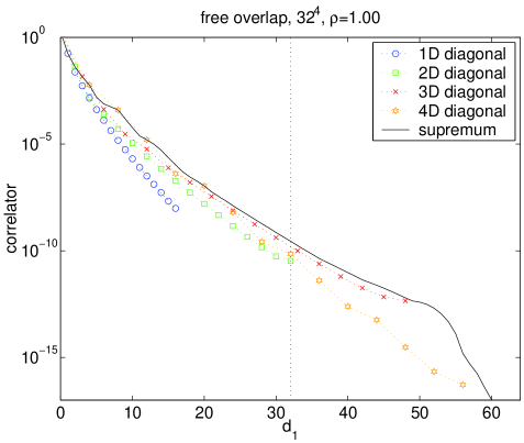
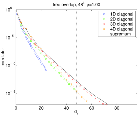
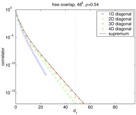
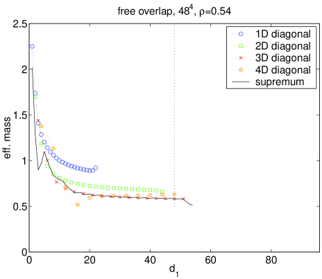
Figure 23: Free overlap couplings in four directions and the function (9) together with their “effective masses” for ($32^{4}$, $\rho\!=\!1$) and ($48^{4}$, $\rho\!=\!1$). Some effective masses are missing, since correlator values below $10^{-17}$ have been cut off (double precision limit). The good agreement of the $32^{4}$ and $48^{4}$ data with evaluation point $d_{1}\!=\!L$ (dotted vertical lines) suggests that these data are much less affected by finite size effects than those near the maximal $d_{1}\!=\!2L$. The correlator with $\rho\!=\!0.54$ is visibly steeper.

Considering $f(d_{1})$ as given in (9) [30] on a finite lattice one encounters a technical problem that is evident in Fig. 23. The free field case is far from showing rotational symmetry and the supremum function (9) has a couple of initial bumps (in particular at $d_{1}\!=\!4,8,12$), and this means that one needs to go to sufficiently large distances to measure the slope in a logarithmic representation. On the other hand, the choice to measure the distance in the 1-norm leads to rather large finite size effects for $d_{1}\!>\!L$, in particular the region near the maximal distance $d_{1}\!=\!2L$ is heavily contaminated. Therefore, we tried

$$\nu={1\over 2}\log(f(L\!-\!1)/f(L\!+\!1))$$ (29)

as a technical definition of the localization $\nu$ in (8). The comparison between the $32^{4}$ and $48^{4}$ geometries shows that our choice to evaluate the logarithmic derivative at $d_{1}\!=\!L$ produces rather consistent $\nu$ values, and we take this as a sign that they cannot be far from the asymptotic exponent. For the (two-digit-precision) projection parameter that we find to be optimal w.r.t. locality in the free case, $\rho_{\mathrm{opt}}^{\mathrm{free}}\!\simeq\!0.54$, the correlator is explicitly shown to be steeper than in the $\rho\!=\!1$ case.

References

- [1]
- [2]
- [3] D.B. Kaplan, Phys. Lett. B 288, 342 (1992) [hep-lat/9206013].
- [4] Y. Shamir, Nucl. Phys. B 406, 90 (1993) [hep-lat/9303005].
- [5] R. Narayanan and H. Neuberger, Nucl. Phys. B 412, 574 (1994) [hep-lat/9307006]. R. Narayanan and H. Neuberger, Nucl. Phys. B 443, 305 (1995) [hep-th/9411108]. H. Neuberger, Phys. Lett. B 417, 141 (1998) [hep-lat/9707022]. H. Neuberger, Phys. Lett. B 427, 353 (1998) [hep-lat/9801031].
- [6] P.H. Ginsparg and K.G. Wilson, Phys. Rev. D 25, 2649 (1982).
- [7] M. Lüscher, Phys. Lett. B 428, 342 (1998) [hep-lat/9802011].
- [8] P. Hasenfratz, V. Laliena and F. Niedermayer, Phys. Lett. B 427, 125 (1998) [hep-lat/9801021].
- [9] F. Niedermayer, Nucl. Phys. Proc. Suppl. 73, 105 (1999) [hep-lat/9810026].
- [10] M. Albanese et al. [APE Collab.], Phys. Lett. B 192, 163 (1987).
- [11] A. Hasenfratz and F. Knechtli, Phys. Rev. D 64, 034504 (2001) [hep-lat/0103029]. A. Hasenfratz, R. Hoffmann and F. Knechtli, Nucl. Phys. Proc. Suppl. 106, 418 (2002) [hep-lat/0110168].
- [12] T. Blum et al., Phys. Rev. D 55, 1133 (1997) [hep-lat/9609036]. G.P. Lepage, Phys. Rev. D 59, 074502 (1999) [hep-lat/9809157]. K. Orginos, D. Toussaint and R.L. Sugar [MILC Collab.], Phys. Rev. D 60, 054503 (1999) [hep-lat/9903032].
- [13] S. Dürr, C. Hoelbling and U. Wenger, Phys. Rev. D 70, 094502 (2004) [hep-lat/0406027].
- [14] S. Dürr and C. Hoelbling, Phys. Rev. D 69, 034503 (2004) [hep-lat/0311002]. S. Dürr and C. Hoelbling, Phys. Rev. D 71, 054501 (2005) [hep-lat/0411022].
- [15] R. Sommer, Nucl. Phys. B 411, 839 (1994) [hep-lat/9310022].
- [16] M. Guagnelli, R. Sommer and H. Wittig [ALPHA Collab.], Nucl. Phys. B 535, 389 (1998) [hep-lat/9806005].
- [17] T. Kalkreuter and H. Simma, Comput. Phys. Commun. 93, 33 (1996) [hep-lat/9507023].
- [18] P. Hernandez, K. Jansen and L. Lellouch, hep-lat/0001008.
- [19] J. Kiskis, R. Narayanan and H. Neuberger, Phys. Lett. B 574, 65 (2003) [hep-lat/0308033].
- [20] S. Dürr, hep-lat/0409141.
- [21] B. Bunk, Nucl. Phys. Proc. Suppl. B 63, 952 (1998) [hep-lat/9805030].
- [22] R.G. Edwards, U.M. Heller and R. Narayanan, Nucl. Phys. B 540, 457 (1999) [hep-lat/9807017].
- [23] J. van den Eshof, A. Frommer, T. Lippert, K. Schilling and H.A. van der Vorst, Comput. Phys. Commun. 146, 203 (2002) [hep-lat/0202025].
- [24] H. Neuberger, Phys. Rev. D 57, 5417 (1998) [hep-lat/9710089].
- [25] A. Borici, Nucl. Phys. Proc. Suppl. 83, 771 (2000) [hep-lat/9909057]. A. Borici, hep-lat/9912040.
- [26] R. Narayanan and H. Neuberger, Phys. Rev. D 62, 074504 (2000) [hep-lat/0005004].
- [27] A. Borici, A.D. Kennedy, B.J. Pendleton and U. Wenger, Nucl. Phys. Proc. Suppl. 106, 757 (2002) [hep-lat/0110070]. U. Wenger, hep-lat/0403003.
- [28] R.C. Brower, H. Neff and K. Orginos, hep-lat/0409118.
- [29] I. Horvath, Phys. Rev. Lett. 81, 4063 (1998) [hep-lat/9808002]. I. Horvath, Phys. Rev. D 60, 034510 (1999) [hep-lat/9901014]. W. Bietenholz, hep-lat/9901005.
- [30] P. Hernandez, K. Jansen and M. Lüscher, Nucl. Phys. B 552, 363 (1999) [hep-lat/9808010].
- [31] T.G. Kovacs, hep-lat/0111021. T.G. Kovacs, Phys. Rev. D 67, 094501 (2003) [hep-lat/0209125].
- [32] H. Neuberger, Phys. Rev. D 61, 085015 (2000) [hep-lat/9911004].
- [33] Y. Kikukawa, Nucl. Phys. B 584, 511 (2000) [hep-lat/9912056].
- [34] K. Fujikawa and M. Ishibashi, Nucl. Phys. B 605, 365 (2001) [hep-lat/0102012].
- [35] D.H. Adams, Phys. Rev. D 68, 065009 (2003) [hep-lat/9907005]. D.H. Adams and W. Bietenholz, Eur. Phys. J. C 34, 245 (2004) [hep-lat/0307022]. D.H. Adams, Nucl. Phys. Proc. Suppl. 129, 513 (2004) [hep-lat/0309148].
- [36] T.W. Chiu, Phys. Lett. B 552, 97 (2003) [hep-lat/0211032].
- [37] L. Giusti, C. Hoelbling and C. Rebbi, Nucl. Phys. Proc. Suppl. 83 (2000) 896 [hep-lat/9906004].
- [38] W. Kerler, Chin. J. Phys. 38 (2000) 623 [hep-lat/9912022]. I. Hip, T. Lippert, H. Neff, K. Schilling and W. Schroers, Phys. Rev. D 65, 014506 (2002) [hep-lat/0105001]. I. Hip, T. Lippert, H. Neff, K. Schilling and W. Schroers, Nucl. Phys. Proc. Suppl. 106, 1004 (2002) [hep-lat/0110155].
- [39] M. Lüscher, S. Sint, R. Sommer and P. Weisz, Nucl. Phys. B 478, 365 (1996) [hep-lat/9605038].
- [40] L. Giusti, C. Hoelbling and C. Rebbi, Phys. Rev. D 64, 114508 (2001) [Erratum-ibid. D 65, 079903 (2002)] [hep-lat/0108007].
- [41] F. Berruto, N. Garron, C. Hoelbling, L. Lellouch, C. Rebbi and N. Shoresh, Nucl. Phys. Proc. Suppl. 129, 471 (2004) [hep-lat/0310006].
- [42] Y. Kikukawa and A. Yamada, hep-lat/9810024.
- [43] C. Alexandrou, E. Follana, H. Panagopoulos and E. Vicari, Nucl. Phys. B 580, 394 (2000) [hep-lat/0002010].
- [44] C.W. Bernard and T. DeGrand, Nucl. Phys. Proc. Suppl. 83, 845 (2000) [hep-lat/9909083].
- [45] T. DeGrand, Phys. Rev. D 67, 014507 (2003) [hep-lat/0210028].
- [46] P. Hasenfratz, S. Hauswirth, K. Holland, T. Jörg, F. Niedermayer and U. Wenger, Int. J. Mod. Phys. C 12, 691 (2001) [hep-lat/0003013]. P. Hasenfratz, S. Hauswirth, T. Jörg, F. Niedermayer and K. Holland, Nucl. Phys. B 643, 280 (2002) [hep-lat/0205010].
- [47] W. Bietenholz, Eur. Phys. J. C 6, 537 (1999) [hep-lat/9803023]. W. Bietenholz and I. Hip, Nucl. Phys. B 570, 423 (2000) [hep-lat/9902019]. W. Bietenholz, Nucl. Phys. B 644, 223 (2002) [hep-lat/0204016]. W. Bietenholz and S. Shcheredin, hep-lat/0502010.
- [48] C. Gattringer and I. Hip, Phys. Lett. B 480, 112 (2000) [hep-lat/0002002]. C. Gattringer, Phys. Rev. D 63, 114501 (2001) [hep-lat/0003005]. C. Gattringer, I. Hip and C.B. Lang, Nucl. Phys. B 597, 451 (2001) [hep-lat/0007042].
- [49] T. DeGrand [MILC Collab.], Phys. Rev. D 60, 094501 (1999) [hep-lat/9903006].
- [50] T. DeGrand [MILC Collab.], Phys. Rev. D 63, 034503 (2001) [hep-lat/0007046]. T. DeGrand, A. Hasenfratz and T.G. Kovacs, Phys. Rev. D 67, 054501 (2003) [hep-lat/0211006].
- [51] W. Kamleh, D.H. Adams, D.B. Leinweber and A.G. Williams, Phys. Rev. D 66, 014501 (2002) [hep-lat/0112041].
- [52] M. Lin [RBC Collab.], hep-lat/0409115.
- [53] K.C. Bowler, B. Joo, R.D. Kenway, C.M. Maynard and R.J. Tweedie [UKQCD Collab.], hep-lat/0411005.
- [54] F.D.R. Bonnet, R.G. Edwards, G.T. Fleming, R. Lewis and D.G. Richards [LHP Collab.], hep-lat/0411028.
- [55] S.R. Beane, P.F. Bedaque, K. Orginos and M.J. Savage [NPLQCD Collab.], hep-lat/0506013.
- [56] A. Ali Khan et al. [CP-PACS Collab.], Nucl. Phys. Proc. Suppl. 94, 725 (2001) [hep-lat/0011032].
- [57] Y. Aoki et al., Phys. Rev. D 69, 074504 (2004) [arXiv:hep-lat/0211023].
- [58] K. Jansen and K.-I. Nagai, JHEP 0312, 038 (2003) [hep-lat/0305009].
- [59] C. Morningstar and M.J. Peardon, Phys. Rev. D 69, 054501 (2004) [hep-lat/0311018].
- [60] T. DeGrand, private communication.
- [61] Z. Fodor, S. D. Katz and K. K. Szabo, JHEP 0408, 003 (2004) [hep-lat/0311010]. T. DeGrand and S. Schaefer, Phys. Rev. D 71, 034507 (2005) [hep-lat/0412005]. N. Cundy, S. Krieg, G. Arnold, A. Frommer, T. Lippert and K. Schilling, hep-lat/0502007. A.D. Kennedy, Nucl. Phys. Proc. Suppl. 140, 190 (2005) [hep-lat/0409167].
- [62] S. Aoki, Phys. Rev. D 30, 2653 (1984).
- [63] E.M. Ilgenfritz, W. Kerler, M. Müller-Preussker, A. Sternbeck and H. Stüben, Phys. Rev. D 69, 074511 (2004) [hep-lat/0309057].
- [64] K.M. Bitar, U.M. Heller and R. Narayanan, Phys. Lett. B 418, 167 (1998) [hep-th/9710052].
- [65] S.R. Sharpe and R.L. Singleton, Phys. Rev. D 58, 074501 (1998) [hep-lat/9804028].
- [66] M. Golterman and Y. Shamir, Phys. Rev. D 68, 074501 (2003) [hep-lat/0306002].
- [67] M. Golterman, S. Sharpe and R.L. Singleton, hep-lat/0501015.