Abstract

Due to its complex structure the parametrized fixed point action can not be simulated with the available local updating algorithms. We constructed, coded, and tested an updating procedure with 2+1 light flavors, where the targeted $s$ quark mass is at its physical value while the $u$ and $d$ quarks should produce pions lighter than $300\,$MeV. In the algorithm a partially global gauge update is followed by several accept/reject steps, where parts of the determinant are switched on gradually in the order of their expenses. The trial configuration that is offered in the last, most expensive, stochastic accept/reject step differs from the original configuration by a Metropolis + over-relaxation gauge update over a sub-volume of $\sim(1.3\,\mathrm{fm})^{4}$. The acceptance rate in this accept/reject step is $\sim 0.4$. The code is optimized on different architectures and is running on lattices with $L_{s}\approx 1.2\,\mathrm{fm}$ and $1.8\,\mathrm{fm}$ at a resolution of $a\approx 0.15\,\mathrm{fm}$.

PACS number: 11.15.Ha, 12.38.Gc, 12.38.Aw

I introduction

There is a considerable freedom in formulating QCD on the lattice. This freedom is reflected in the large number of actions tested and used in the quenched approximation. There are no miracles: good scaling, good chiral properties, theoretical safety and the expenses are in balance. Short of an algorithmic breakthrough one can expect to see in the future a plethora of full QCD simulations and results obtained with different formulations adapted to the physical problem as it happened in the quenched approximation.

In this paper we discuss a full QCD algorithm for 2+1 light flavors with the parametrized fixed point action Hasenfratz et al. (2001); Niedermayer et al. (2001); Jorg (2002); Hauswirth (2002). The lightest quark mass $m_{ud}$ which can be simulated is set only by the small chiral symmetry breaking caused by the parametrization error, the expenses of a full updating sweep are practically independent of $m_{ud}$.

Our updating procedure has no special problems in connecting different topological sectors nor in suppressing the topological susceptibility. The algorithm is exact and the action certainly describes QCD in the continuum limit. It is a partially global update where the pieces of the determinant are switched on gradually in the order of their expenses. The partially global update implies that this is a volume-squared algorithm which constraints the size of lattices one can cope with in the simulations. Actually, the expense of a specific section of the algorithm, the eigenvalue solver, increases even faster with the volume, but in the present simulations this part is not dominating.

In the ongoing runs the target spatial sizes are $L_{s}\approx 1.2\,$fm and $1.8\,$fm with a resolution $a\approx 0.15\,$fm. The target pion mass is below $300\,$MeV. On the $1.2\,$fm lattice we also ran with the smallest $m_{ud}$ quark mass which can be treated with our Dirac operator, basically with massless quarks.

Actions which approximate the fixed point of a renormalization group transformation have been tested in detail in $d=2$ and $d=4$. The present form of the QCD fixed point action and the related codes are the result of a long development to which many of our colleagues contributed (see Ref. Gattringer et al. (2004) and references therein). The algorithm discussed here is optimized and running on three different platforms (IBM SP4, PC Cluster, Hitachi SR8000). This paper is organized as follows. In Sect.II we briefly describe the fixed point action. Sect.III summarizes the Partial Global Stochastic Update and its improvements in a general form while Sect.IV describes how the update is implemented in our simulation. In Sect.V we present some numerical results that illustrate the updating algorithm.

II The Action

II.1 The parametrized fixed point action

The special QCD action which is the fixed point of a renormalization group transformation has several desirable properties Hasenfratz and Niedermayer (1994). It is a local solution of the Ginsparg-Wilson equation Ginsparg and Wilson (1982),

$$\gamma_{5}D+D\gamma_{5}=D\gamma_{5}2RD,$$ (1)

with a non-trivial local matrix $R$ which lives on the hypercube Hasenfratz (1998). The quark mass is introduced as

$$D(m)=D+m\left(\frac{1}{2R}-\frac{1}{2}D\right).$$ (2)

Eq.1 guarantees that the Dirac operator is chirally invariant. Since it is the fixed point of a renormalization group transformation, it has no cut-off effects in the classical limit. The parametrized version of this action is an approximation which has been carefully tested in the classical limit and in quenched simulations Hasenfratz et al. (2002a, b); Gattringer et al. (2004); Hasenfratz et al. (2004).

The parametrized fixed point gauge action $S_{g}(U)$ Niedermayer et al. (2001) is a function of plaquette traces built from the original gauge links $U$, and from smeared links. The smeared link contains staples in an asymmetric way: the weights of staples which lie in, or orthogonal to the plane of the plaquette are different. The gauge action is a polynomial of smeared and unsmeared plaquette traces. The 5 non-linear and 14 linear parameters are fitted to the fixed point action.

The Dirac operator Hasenfratz et al. (2001); Hasenfratz et al. (2002c) is constructed on smeared gauge configurations $V(U)$. This smearing is local and contains links projected to SU(3). It is constructed using renormalization group considerations DeGrand et al. (1998) and it reflects the discontinuous character of the chiral Dirac operator when the topological charge changes Jorg (2002). The Dirac operator has fermion offsets on the hypercube only. In Dirac space all the elements of the Clifford algebra enter. The structure of these terms is restricted by the symmetries $C$, $P$, $\gamma_{5}$-hermiticity, and cubic symmetry. The 82 free coefficients of this Dirac operator are determined by a fit to the fixed point Dirac operator. We note that also for the Chirally Improved Dirac operator – which has a similarly complex structure – a global update has been suggested in Ref. Lang et al. (2004)

II.2 The 2+1 flavor action

Our goal is to simulate a $2+1$ flavor system with quark masses close to their physical values. As usual we integrate out the the fermionic fields and write the action as

$$S = \beta S_{g}(U)+\bar{u}D(m_{ud})u+\bar{d}D(m_{ud})d+\bar{s}D(m_{s})s$$ (3)

$$\simeq \beta S_{g}(U)-\ln{\rm{det}^{2}}{D(m_{ud})}-\ln\det{D(m_{s})}.$$ (4)

The $\gamma_{5}$-hermiticity of the Dirac operator ensures that $\det{D(m)}$ is real, $\det{D(m)}=\det{D^{\dagger}(m)}.$ If $D$ were an exact solution of Eq.1 then $\det{D(m)}$ would be positive for any $m>0$. Due to parametrization errors our Dirac operator has no exact chiral symmetry and the requirement of $\det{D(m)}>0$ puts a constraint on the quark mass $m$. For now we assume that this condition is satisfied.

One can rewrite the action in an explicitly Hermitian form

$$S=\beta S_{g}(U)-\ln{\det{(D^{\dagger}(m_{ud})D(m_{ud}))}}-\ln{\det{\left(\sqrt{D^{\dagger}(m_{s})}\sqrt{D(m_{s})}\right)}}\,.$$ (5)

We want to emphasize that the appearance of the square root in Eq.5 does not mean that we simulate a possibly non-local action. The action we simulate is given by the manifestly local form in Eq.3.

III The Stochastic Update and its Improvements

The parametrized fixed point action contains many gauge paths and SU(3) projections. It is too complicated, if not impossible, to simulate with algorithms that would require the derivative of the action with respect of the gauge fields. For that reason we have adapted an updating method that requires only a stochastic estimate of the action at each step. The (Partial) Global Stochastic Update was developed in Hasenfratz and Knechtli (2002), based on an old suggestion Grady (1985); Creutz (1992), to simulate smeared link staggered actions. It was developed further in Hasenfratz and Alexandru (2002); Alexandru and Hasenfratz (2002); Knechtli and Wolff (2003). Stochastic or “noisy” updating algorithms have been used in different context by many other groups Kennedy and Kuti (1985); Kennedy et al. (1988); Joo et al. (2003); Montvay and Scholz (2005). Here we take over the main points of the Global Stochastic Update but add several improvements to create an efficient updating algorithm. In the next section we will summarize the general ideas of the update, then discuss the specific improvements we have implemented.

III.1 The Partial-Global Stochastic Update

In order to simplify the notation in this section we consider an action with the generic form

$$S=\beta S_{g}(U)-\ln{\det{A^{\dagger}A}}.$$ (6)

Here $A^{\dagger}A$ describes 1 or 2 flavors of massive fermions as discussed in Sect.II.2. A Global Update proceeds in two steps:

• Update (a part of) the configuration $U\to U^{\prime}$ with the gauge action $\beta S_{g}$ using Metropolis, over-relaxation or other updates.

One could accept or reject (A/R) the proposed $U^{\prime}$ configuration with probability

$$P_{{\rm{acc}}}={\rm{min}\left(1,\frac{\det A^{\prime\dagger}A^{\prime}}{\det A^{\dagger}A}\right).}$$ (7)

This procedure clearly satisfies the detailed balance condition but requires the evaluation of the fermionic determinant. This lengthy calculation can be replaced by a stochastic estimator as follows. We write the determinant ratio as a stochastic integral

$$\frac{\det A^{\prime\dagger}A^{\prime}}{\det A^{\dagger}A} = \det{(\Omega{}^{\dagger}\Omega)^{-1}}$$ (8)

$$\simeq \int D[\eta^{\dagger}\eta]e^{-\eta^{\dagger}\eta}e^{-(\eta^{\dagger}\Omega^{\dagger}\Omega\eta-\eta^{\dagger}\eta)}$$

where we introduced the notation

$$\Omega=A^{\prime-1}A\,.$$ (9)

• For the stochastic accept/reject step we first create a Gaussian random vector $\eta$ with $P(\eta)\propto\exp(-\eta^{\dagger}\eta)$. Now the new configuration is accepted with the probability

  $$P_{{\rm{acc}}}^{{\rm{stoch}}}=\min{(1,e^{-\Delta S_{f}})},$$ (10)

  where

  $$\Delta S_{f}=\eta^{\dagger}(\Omega^{\dagger}\Omega-1)\eta.$$ (11)

  Eq.11 defines the stochastic estimator $\Delta S_{f}$, the change of the fermionic action with fixed $\eta$ Hasenfratz and Knechtli (2002).

The stochastic update satisfies the detailed balance condition Grady (1985); Creutz (1992); Alexandru and Hasenfratz (2002), and repeating steps A-B creates a sequence of gauge configurations with the proper probability distribution.

For the 2+1 flavor system of Eq.5 the stochastic estimator contains two terms

$$\Delta S_{f}=\eta_{u}^{\dagger}(\Omega_{ud}^{\dagger}\Omega_{ud}-1)\eta_{u}+\eta_{s}^{\dagger}(\Omega_{s}^{\dagger}\Omega_{s}-1)\eta_{s}$$ (12)

with $\Omega_{ud}=D^{\prime}\,{}^{-1}(m_{ud})D(m_{ud})$ and $\Omega_{s}=\sqrt{D^{\prime-1}(m_{s})}\sqrt{D(m_{s})}$.

The main ideas of the stochastic Monte Carlo update has been known for a long time but it has not been used in numerical simulations because of technical difficulties. In its original form the acceptance rate in Eq.10 is infinitesimally small unless the configurations $U$ and $U^{\prime}$ are nearly identical. The root of this problem is two-fold.

On one hand, if the typical values of $|\log\det(D^{\prime}/D)|$ are significantly larger than 1 the acceptance rate will be very small, even if the determinant ratio was calculated deterministically. On the other hand, an additional suppression of the acceptance rate occurs due to the stochastic evaluation in the A/R step. To illustrate this consider the case when $\det D^{\prime}/\det D=1$. Take a simple model for this situation with a Gaussian random variable $P(x)\propto\exp(-(x-x_{0})^{2}/2\sigma^{2})$. The relation $\langle\mathrm{{e}^{-x}\rangle=1}$ implies $x_{0}=\sigma^{2}/2$ hence for large $\sigma$ the acceptance rate is extremely small, $\sim\mathrm{e^{-\sigma^{2}/2}\ll 1}$.

Note that the standard deviation of $\exp(-\eta^{\dagger}(\Omega^{\dagger}\Omega-1)\eta)$ is infinite if any of the eigenvalues of $\Omega=A^{\prime-1}A$ is smaller than $1/2$ Alexandru and Hasenfratz (2002). However, the extremely small acceptance rate occurs much before this bound is reached. In the following we discuss four improvement steps which are essential to get an algorithm with a good acceptance rate.

III.2 Improvements of the Global Stochastic Update

In this section we discuss the different improvements we implemented to increase the effectiveness of the stochastic updating. In the reduction technique the UV part of the determinant is separated, its value is calculated non-stochastically and taken into account more frequently by intermediate A/R steps. This increases the acceptance rate in the stochastic A/R step significantly by reducing both problems mentioned above. The subtraction technique separates the IR modes by calculating the eigenvalues and eigenvectors of the first few low eigenmodes of the Dirac operator. It acts analogously for the IR modes as the reduction for the UV part. The last two techniques, the relative gauge fixing and the determinant breakup, are applied in the last, stochastic A/R step, and are aimed at reducing the fluctuations. The relative gauge fixing brings the configuration $U^{\prime}$ as close to $U$ as possible. The determinant breakup rewrites the Dirac operator as product of operators. The stochastic estimator becomes a sum of independent terms and its fluctuation is reduced.

The Global Stochastic Monte Carlo Update would not be effective without these improvements. On large lattices even with the improvements one can update only a part of the configuration before evaluating the stochastic estimator making the algorithm to scale with the square of the volume. Nevertheless on moderate volumes we found the algorithm effective, allowing the dynamical simulation of light, even nearly massless, quarks with an action where the chiral breaking and lattice artifacts are small.

III.2.1 The Reduction:

The stochastic change of the fermionic action can be written as $\Delta S_{f}=\sum_{i}(\omega_{i}-1)\eta_{i}^{\dagger}\eta_{i}$ where $\omega_{i}$ are the real eigenvalues of the operator $\Omega^{\dagger}\Omega$ and $\eta_{i}^{\dagger}\eta_{i}=O(1)$. While the eigenvalues of the Dirac operator are restricted to a compact region, $\omega_{i}$ can vary between $\sim m$ to $\sim 1/m$, though most of the eigenvalues correspond the the UV modes are $O(1)$. These UV modes contribute little to $\Delta S_{f}$ individually, but there are so many of them that they dominate the fluctuations. To reduce the fluctuations we transform the Dirac operator $D\to D_{r}$ such that the UV modes of $D_{r}$ are condensed and thus the corresponding eigenmodes of $\Omega$ are closer to unity. We choose $D_{r}$ such that the change in the determinant $\det(D/D_{r})$ is calculable analytically (non-stochastically).

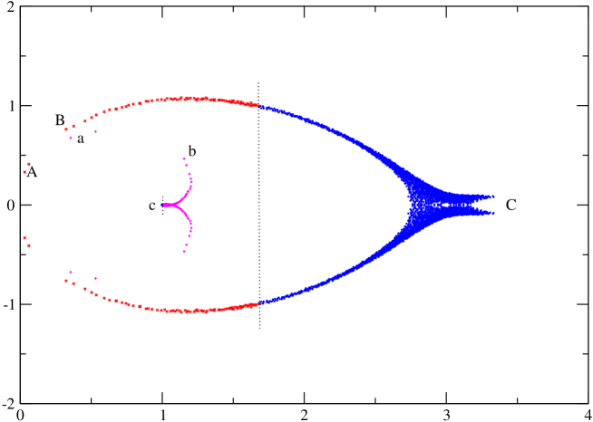
Figure 1: The eigenvalue spectrum of the Dirac operator on a single $4^{4}$ gauge configuration. The points of the larger “Batman” like figure correspond to the original Dirac operator while the points of the smaller “wing-shape” structure in the center represent the corresponding eigenvalues of the reduced Dirac operator $D_{r}/s$. Sections marked by $A$, $B$ and $C$ on the original spectrum are mapped to sections $a$, $b$ and $c$ after reduction.

The effect of the reduction on the eigenvalue spectrum of $D$ is illustrated in Figure 1. The spectrum was calculated on a single $4^{4}$ quenched gauge configuration $U$ with $a\approx 0.15\,$fm in Jorg (2002). The larger “Batman” like structure corresponds to the spectrum of the original Dirac operator. The “Batman ears” are mainly the consequence of the non-trivial $R$ operator and are strongly reduced if one considers the spectrum of $DR$ which is close to a circle. An overwhelming part of the eigenvalues are around the $UV$ point $(s,0)$ in the complex plane where $s\approx 2.8$. The points to the right of the long dotted line represent 95% of the eigenvalues. With the reduction we attempt to move the eigenvalues of $D/s$ close to $1$. Following Refs. de Forcrand (1999); Hasenbusch (2001); Hasenfratz and Knechtli (2002) we define a reduced Dirac operator

$$D_{r}=D\,e^{-\sum_{i=1}^{n}c_{i}(D/s-1)^{i}}.$$ (13)

Choosing the coefficients $c_{i}=(-1)^{i+1}/i$ the reduced operator is $D_{r}/s=1+O((D/s-1)^{n+1})$. The ratio of the determinants $D_{r}$ and $D$ can be expressed in terms of traces of $D$

$$\det D_{r} = \det D\,e^{-\sum_{i=1}^{n}c_{i}Tr(D/s-1)^{i}}$$ (14)

$$= \det D\,e^{-\sum_{i=1}^{n}\alpha_{i}TrD^{i}}\,,$$

and can be calculated non-stochastically by evaluating $\mathop{\hbox{Tr}}D^{k}$, $k=1,n$. The computing time and the complexity of the code to do the trace calculations increase rapidly as $n$ increases. With our Dirac operator we decided to stop at $n=4$ in the reduction. Working with $D_{r}$ is not much different from $D$. Both in multiplication and inversion the exponential term in Eq.13 can be approximated by a relatively low order polynomial.

In Figure 1 the smaller wing-shape object in the center corresponds to the eigenvalues of $D_{r}/s$ on the same gauge configuration as before. Sections marked as $A$, $B$ and $C$ on the original spectrum are mapped to sections $a$, $b$ and $c$ after reduction, illustrating how the eigenvalues are transformed. The origin is a stationary point. The main effect of the reduction is condensing the UV modes. The points to the left of the short dotted line again represent 95% of the eigenvalues. This region is not very obvious in the figure since all its points are contained in a circle around $(1,0)$ with radius of about 0.01 (with the overwhelming part of the eigenvalues being much closer), showing the strength of the reduction. Accordingly, the $UV$ fluctuations, that is the contribution of the UV modes to the stochastic estimator $\Delta S_{f}$, is greatly reduced.

At this point the action Eq.5 can be written as

$$S = \beta S_{g}(U)+S_{UV}$$ (15)

$$- \ln{\det{D_{r}^{\dagger}(m_{ud})D_{r}(m_{ud})}}-\ln{\det{D_{r}(m_{s})}}$$

where

$$S_{UV}=-2\sum_{i=1}^{n}\alpha_{i}\mathop{\hbox{Tr}}{D^{i}(m_{ud})}-\sum_{i=1}^{n}\alpha_{i}\mathop{\hbox{Tr}}{D^{i}(m_{s})}$$ (16)

carries most of the UV part of the determinant.

III.2.2 The Subtraction

The reduction of the Dirac operator as discussed in the previous section effects mainly the non-physical UV part of the determinant. The subtraction that we introduce here deals with the low lying IR eigenvalues of the Dirac operator. The small eigenvalues of $D^{\prime}$ can create large $\omega_{i}$ eigenvalues of $\Omega=D^{\prime}\,{}^{-1}D$. Besides suppressing such configurations in the (full QCD) equilibrium configurations, their presence produces large fluctuations in the stochastic estimator, reducing therefore the acceptance rate in the stochastic A/R step. By calculating some low lying eigenvalues (and the corresponding eigenvectors) one can take into account their contribution more frequently and deterministically, so they do not participate in the stochastic A/R step.

Denote the right and left eigenvectors of the Dirac operator by

$$Dv_{\lambda}=\lambda v_{\lambda}\,,\qquad w_{\lambda}^{\dagger}D=\lambda w_{\lambda}^{\dagger}\,.$$ (17)

The eigenvectors $w_{\lambda}^{\dagger}$ can be chosen to fulfill the normalization condition

$$w_{\lambda}^{\dagger}v_{\lambda^{\prime}}=\delta_{\lambda\lambda^{\prime}}\,.$$ (18)

In terms of the (non-hermitian) projector operators

$$P_{\lambda}=v_{\lambda}w_{\lambda}^{\dagger}\,$$ (19)

which, due to Eq.18, satisfy the relation $P_{\lambda}^{2}=P_{\lambda}$, the Dirac operator can be written as

$$D=\sum\lambda P_{\lambda}\,.$$ (20)

The subtracted Dirac operator is defined by replacing a set of the lowest eigenvalues by the constant $s$

$$D_{s}=D+\sum_{{\rm{low}}}(s-\lambda)P_{\lambda}\,.$$ (21)

We assume that we subtract the complex conjugate pairs together. For an arbitrary analytic function $f(D)$ the subtraction gives

$$f(D_{s})=f(D)+\sum_{{\rm{low}}}(f(s)-f(\lambda))P_{\lambda}.$$ (22)

Subtracting the reduced Dirac operator of Eq. 13 gives then

$$D_{rs}=D\mathrm{e}^{-\sum_{i}c_{i}(D/s-1)^{i}}+\sum_{{\rm{low}}}\left(s-\lambda\mathrm{e}^{-\sum_{i}c_{i}(\lambda/s-1)^{i}}\right)P_{\lambda}\,.$$

The small eigenvalues of the subtracted, reduced $D_{rs}$ operator are replaced by $s$ while its UV part is condensed near $s$. The stochastic estimator of $D_{rs}$ has reduced fluctuations and reduced absolute value as well.

The ratio of the determinants of $D_{rs}$ and $D_{r}$ can be calculated analytically using the relation

$$\det D_{r}=\det D_{rs}\prod_{{\rm{low}}}\frac{\lambda}{s}e^{-\sum_{i}c_{i}(\lambda/s-1)^{i}}\,.$$ (23)

The inversion of $D$ using that of $D_{s}$ is given by

$$D^{-1}=\left[1+\sum_{{\rm{low}}}\left(\frac{s}{\lambda}-1\right)P_{\lambda}\right]D_{s}^{-1}\,.$$ (24)

The smallest eigenvalues of $D$ are replaced by the constant $s$ in $D_{s}$ therefore the conjugate gradient method converges faster for $D_{s}$.

At this point the action of Eqs.5 and 15 can be written as

$$S = \beta S_{g}(U)+S_{UV}+S_{IR}$$ (25)

$$- \ln{\det{D_{rs}^{\dagger}(m_{ud})D_{rs}(m_{ud})}}-\ln{\det{D_{rs}(m_{s})}}$$

where

$$S_{IR} = 2\sum_{{\rm{low}}}\left(-\ln\frac{|\lambda_{ud}|}{s}+\sum_{i}c_{i}\left(\frac{\lambda_{ud}}{s}-1\right)^{i}\right)$$ (26)

$$+ \sum_{{\rm{low}}}\left(-\ln\frac{|\lambda_{s}|}{s}+\sum_{i}c_{i}\left(\frac{\lambda_{s}}{s}-1\right)^{i}\right)\,.$$

III.2.3 The Relative Gauge Fixing

Even if $U^{\prime}$ is a gauge transform of $U$, hence the determinant ratio is exactly 1, the eigenvalues of $\Omega=D(U^{\prime})^{-1}D(U)$ are in general different from 1 (only their product is 1). As a consequence the stochastic estimator in the A/R step can have large fluctuations, greatly reducing the acceptance rateKnechtli and Wolff (2003). These fluctuations can be reduced significantly by gauge transforming $U^{\prime}$ so as to maximize $\mathrm{\sum_{x,\mu}{Re}\mathrm{{Tr}(U^{\prime}_{x\mu}U_{x\mu}^{\dagger})}}$, i.e. by bringing $U^{\prime}$ as close to $U$ as possible. (We have also tried to fix the gauge in both $U$ and $U^{\prime}$ by some given “absolute” gauge fixing condition, but the method discussed above was more efficient.)

III.2.4 The Determinant Breakup

The reduction, subtraction, and relative gauge fixing result in significant improvement of the stochastic estimator. Further improvements can be achieved by writing the Dirac operator as the product of $l$ terms

$$A=A_{1}\times A_{2}\times....\times A_{l}\,.$$ (27)

The corresponding stochastic estimator is the sum of $l$ terms

$$\Delta S_{f}=\sum_{i=1}^{l}\eta_{i}^{\dagger}(\Omega_{i}^{\dagger}\Omega_{i}-1)\eta_{i}$$ (28)

with $l$ stochastic $\eta$ vectors and $\Omega_{i}=A^{\prime}_{i}\,{}^{-1}A_{i}$. If the eigenspectrum of the individual $A_{i}$ operators is closer to a constant the fluctuation of the stochastic estimator is reduced. In Refs. Alexandru and Hasenfratz (2002, 2003), following a suggestion in Ref. Hasenbusch (1999), the terms in Eq.27 were chosen to be identical, $A_{i}=A^{1/l}$. While this choice does reduce the fluctuations, it creates $l$ equally singular terms and requires the calculation of the $l$th root for each of them. We found it is more effective to generalize the mass shifting method of Hasenbusch (2001) and write the Dirac operator as

$$\frac{1}{s}A=\frac{A(\mu_{0})}{A(\mu_{1})}\times\frac{A(\mu_{1})}{A(\mu_{2})}\times...\times\frac{A(\mu_{l-1})}{A(\mu_{l})}\times A(\mu_{l})\,,$$ (29)

where $A(\mu)=\frac{1}{s+\mu}(A+\mu)$ and $\mu_{0}=0$. The mass shift values $\mu_{i}$ are chosen such that each term in $\Delta S_{f}$ contributes approximately equally.

The first term in Eq.28 is the easiest to analyze. At lowest order in $\mu_{1}$

$$\eta_{1}^{\dagger}(\Omega_{1}^{\dagger}\Omega_{1}-1)\eta_{1}=-\eta_{1}^{\dagger}\left(\frac{\mu_{1}}{A}+\frac{\mu_{1}}{A^{\dagger}}-\frac{\mu_{1}}{A^{\prime}}-\frac{\mu_{1}}{A^{\prime}\,{}^{\dagger}}\right)\eta+O(\mu_{1}^{2})\,.$$ (30)

Unless the operators $A$ and $A^{\prime}$ are close to each other, $\mu_{1}/A$ has to be small to control the stochastic fluctuations. Consequently $\mu_{1}$ has to be much smaller than the smallest eigenvalue of $A$. Later terms allow larger change in the shift masses $\mu_{i}$. The last mass of the series, $\mu_{l}$, is chosen such that the stochastic estimator of the single operator $A(\mu_{l})$ is comparable to the previous terms. It is interesting to note that the leading term in Eq.30 vanishes for a Ginsparg-Wilson Dirac operator with $R={\rm{const}}$. However it is not zero in our case.

In practice we combine the reduction, subtraction, relative gauge fixing and the determinant breakup. Only the last two terms of Eq.25 are treated stochastically. For the degenerate $u$ and $d$ quarks we can have

$$A = D_{rs}(m_{ud})\,,$$

$$A(\mu) = \left(\frac{D_{r}(m_{ud})+\mu}{s+\mu}\right)_{s}\,,$$ (31)

where the subtraction is defined as in Eq.22. Each term in the stochastic estimator requires two multiplications and two inversions by $A(\mu)$. For the inversion a standard conjugate gradient or its variant can be used.

For the $s$ quark the situation is slightly more complicated. The $A$ operator contains a square root operation

$$A = \sqrt{D_{rs}(m_{s})}\;,$$

$$A(\mu) = \sqrt{\left(\frac{D_{r}(m_{s})+\mu}{s+\mu}\right)_{s}}\;.$$ (32)

Again, each term in the stochastic estimator requires two multiplications and two inversions by $A(\mu)$. For both of these we approximate the square root operator by a polynomial series. Polynomials have been used to approximate both positive and negative roots of Dirac operators before Montvay (1998); Alexandru and Hasenfratz (2003, 2002). Our situation is different because the operator $D_{r}(m_{s})$ is complex. The case of optimal polynomials for a complex spectrum has been studied in Borici and de Forcrand (1995). Fortunately the strange quark mass is sufficiently heavy and a Taylor expansion in $(D(m)/s-1)$ works well.

IV The Algorithm with 2+1 Flavors

We describe now the algorithm which has been coded, tested and optimized for different platforms.The algorithm starts with a partially global gauge update which is followed by several accept/reject steps, where parts of the determinant are switched on gradually in the order of their expenses. It is convenient to rewrite the action of Eq.25 in a different form

$$S = (\beta+\delta\beta)S_{g}(U)$$

$$+ [S_{UV}^{g}-\delta\beta S_{g}(U)]$$

$$+ [S_{UV}-S_{UV}^{g}+S_{IR}^{{\rm{appr}}}]$$

$$+ [S_{IR}-S_{IR}^{{\rm{appr}}}-\ln{\det{D_{rs}^{\dagger}(m_{ud})D_{sr}(m_{ud})}}-\ln{\det{D_{rs}(m_{s})}}].$$

The meaning of the different terms will be explained in the rest of this section.

IV.1 Gauge update

The gauge update is a standard Metropolis/over-relaxation local update with the fixed point gauge action at coupling $\beta_{{\rm{eff}}}=\beta+\delta\beta$. Here $\delta\beta$ (added at this point and subtracted later) approximates the shift of the gauge coupling due to the determinant and helps to generate configurations with lattice spacing $a$ that is close to the target value already at this step. $4n_{p}$ gauge links, originating from $n_{p}$ consecutive lattice sites, are updated with Metropolis and then the same links with over-relaxation in a reversible sequence. This combination of updates we shall call a ’double update’ in the following.

In the first test runs our target lattice spacing is $a\approx 0.15$ fm and $n_{p}$ is 128 and 144 on the $8^{3}\times 24$ and $12^{3}\times 24$ lattices, respectively. In order to get the resolution $a$ close to the target value we had to tune the coupling $\beta$ repeatedly. The figures in this paper refer to the choice $\beta=3.15$.

IV.2 The 1st accept/reject step

The gauge configuration created as discussed above is accepted/rejected (A/R) with the action $S_{UV}^{g}-\delta\beta S_{g}(U)$, where $S_{UV}^{g}$ is a good gauge approximation to the reduction contribution $S_{UV}$ of Eq.16. The function $S_{UV}^{g}$ is represented by different gauge loops with fitted coefficients on the smeared configuration $V(U)$. This smearing is the same which was used in the parametrized Dirac operator (Sect.II.1). Calculating $S_{UV}^{g}$ is fast and can be done without building up the Dirac operator. The deviation between $S_{UV}^{g}$ and the exact reduction $S_{UV}$ will be corrected in the 2nd accept/reject step below. The parameter $\delta\beta$ is chosen to maximize the acceptance rate in this step.

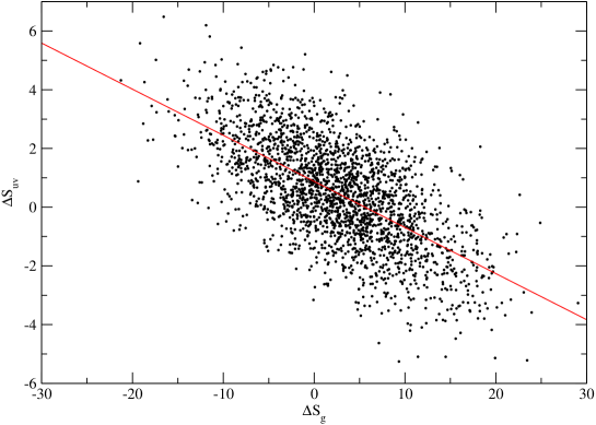
Figure 2: The correlation between $\Delta S_{UV}$ and $\Delta S_{g}$. The slope predicts the optimal value of $\delta\beta\approx 0.15$.

Figure 2 shows the correlation between $\Delta S_{g}$, the change of the gauge action, and $\Delta S_{UV}$, the change of the contribution from the reduction, for a set of configuration pairs $\{U,U^{\prime}\}.$ From the slope $\delta\beta=-0.15$ seems to be a reasonable choice. It is interesting to note that for our action the introduction of the determinant increases the gauge coupling. In the usual Wilson and staggered fermion simulations this shift is larger and in the opposite direction. Since the reduction contribution is large for distant configurations and the $-\delta\beta S_{g}$ term cancels it only approximately, we have to keep the number of updated links $4n_{p}$ in the gauge update modest in order to get a good acceptance rate in this 1st accept/reject. The combination of steps in Sects IV.1 and IV.2 is repeated $N_{1}$ times.

With the $n_{p}$ value quoted before, the 1st acceptance rate is above 0.5. In the running simulations $N_{1}=28$, i.e. $4\times n\times N_{1}\approx 15\mathrm{k}$ links are double updated before the 2nd accept/reject step.

IV.3 The 2nd accept/reject step

The cycle of repeated steps in Sects IV.1 and IV.2 is followed by a 2nd accept/reject decision. In this step the Dirac operator is built on the $U^{\prime}$ competitor configuration, the traces are calculated for the exact reduction, and a certain number of the lowest eigenvalues and eigenvectors are determined. The proposed configuration is accepted/rejected with the action $(S_{UV}-S_{UV}^{g})+S_{IR}^{{\rm{appr}}}$. The first term corrects the small error we made in the 1st A/R step in approximating the traces in $S_{UV}$ with gauge loops. This error is typically small as shown in Figure 3, where the change $\Delta S_{UV}^{g}$ calculated in the gauge approximation is shown as the function of its exact value. (The action differences plotted in this figure are taken between configurations which are offered to the 3rd A/R step, as a result of several 2nd A/R steps. These large values of O(10) would cause a very small acceptance rate in the 3rd step, had we not taken into account this contribution more frequently in the 2nd step.)

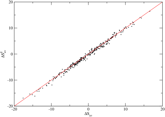
Figure 3: The approximation of $\Delta S_{UV}$ in terms of gauge loops, $\Delta S_{UV}^{g}$. This error is corrected in the 2nd A/R step.

The last term $S_{IR}^{{\rm{appr}}}$ is an approximation to the contribution of the low lying eigenvalues to the determinant $S_{IR}$ in Eq.26. $n_{{\rm{ev}}}$ eigenvalues and the corresponding $S_{IR}$ are calculated for $m_{ud}$ using an Arnoldi eigenvalue finder. The eigenvalues for $m_{s}$ are determined from these, using leading order perturbation theory. (Due to the presence of R in the Ginsparg-Wilson relation, Eq.1, the reaction of the eigenvalues on changing the quark mass is not a simple shift.) This approximation is very good, the error is typically $O(10^{-4})$ . The combination of the steps in Sects.IV.1, IV.2 and IV.3 is repeated $N_{2}$ times.

At present we calculate $n_{{\rm{ev}}}=48$ eigenvalues, which include all the eigenvalues with absolute value below $\approx 0.40$ and $\approx 0.19$ on the $8^{3}\times 24$ and $12^{3}\times 24$ lattices, respectively. The reduction shifts these values further to around $\approx 1.0$ and $\approx 0.5$. We use an Arnoldi routine from the publicly available PARPACK package. The application is far from optimal in our case. Even though the eigenvalues and eigenvectors are calculated on very similar configurations and change little from step to step, the routine cannot use this fact and calculates each eigenvalue set basically independently. The internal calculations of the package are also expensive, the multiplication of a vector by the Dirac operator does not dominate it. These problems limit the number of times the 2nd A/R step is repeated. We can afford $N_{2}=6$ repetitions and the acceptance rate of the 2nd A/R step is around 0.65. Overall about $\approx 90\mathrm{k}$ links are double updated before the 3rd A/R step.

IV.4 The 3rd accept/reject step

The cycle described above is followed by a final, stochastic accept/reject step with the action $S_{IR}-S_{IR}^{{\rm{appr}}}-\ln{\det{D_{rs}^{\dagger}(m_{ud})D_{rs}(m_{ud})}}-\ln{\det{D_{rs}(m_{s})}}$. The first part corrects the small error we made in calculating the contribution of the low lying eigenvalues of $D(m_{s})$ to the determinant in the 2nd A/R step. For that we determine the low lying spectrum of $D(m_{s})$ on the competitor configuration $U^{\prime}$ which is first relative-gauge-fixed with respect to $U$. The second term gives the stochastic estimator of the subtracted, reduced, 2+1 flavor determinant. For the light quarks we break up the determinant into $76$ terms. The lowest eigenvalue of the reduced subtracted Dirac operator, $D_{rs}/s$ is around one and the first few mass shifts have to be much smaller than that (see Sect.III.2.4). We chose $\Delta\mu_{i}=\mu_{i+1}-\mu_{i}=0.01$ for $i=1-20$. The later $\Delta\mu$ values are considerably larger. Due to the subtraction of the low lying eigenmodes the conjugate gradient iteration converges relatively fast, in about 70 steps at the lowest mass shifts and in 5-10 steps at the largest, each step requiring two $D\times v$ Dirac operator multiplications. The exponential term for the reduction requires about 20 $D\times v$ multiplications. For $m_{s}$ the determinant breakup has 38 terms and the smallest shift is $\Delta\mu=0.02$. The square root and its inverse of the reduced, subtracted Dirac operator is approximated by their Taylor series in $(D/s-1)$. In the smaller mass shift region we use 250-300 order polynomials, for the larger mass shift values this reduces to order 30-40. We expect that this section of the code could be significantly improved.

With this closing accept/reject step the algorithm becomes exact. The steps in Sects. IV.1, IV.2, IV.3, and IV.4 are repeated and the accepted configurations that went through all three filters form a Markov chain corresponding the parametrized fixed point action. The acceptance rate of the 3rd A/R step is approximately 0.4.

IV.5 Optimization and performance

The code is optimized on three different platforms (IBM SP4, PC cluster and Hitachi SR8000). The dominating numerical step is the multiplication of a vector by the Dirac operator, $D\times v$, which can be effectively parallelized on all the platforms. The effectiveness of the internal manipulations of the PARPACK package, however, is very sensitive to the architecture. It would be very preferable to replace this part of the code by a QCD specialized piece.

The stochastic estimator (in the 3rd accept/reject) requires $\approx 21\mathrm{k}$ and $\approx 26\mathrm{k}$ $D\times v$ multiplications on the $8^{3}\times 24$ and $12^{3}\times 24$ lattices, respectively. To calculate the first 48 eigenvalues/eigenvectors of the Dirac operator requires $\approx 1\mathrm{k}$ and $\approx 2\mathrm{k}$ $D\times v$ multiplications on the smaller and larger lattices, respectively.

At certain stages of the calculation the processors are divided in two groups and work on the gauge and Dirac part of the code independently. They are joined, however, to calculate the stochastic estimator together.

V Preliminary Results

In our first set of test runs, starting from two different $a\approx 0.15\,$fm quenched configurations, we generated about 400 + 600 $8^{3}\times 24$ configurations, each separated by a full cycle of updates and A/R steps as described in Sects.IV.1-IV.4. We chose the run parameters, based on earlier quenched runs, as $\beta=3.15,$ $\delta\beta=-0.15,$ $m_{ud}=0.017$ and $m_{s}=0.095.$

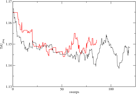
Figure 4: The equilibration of the plaquette as the function of updating sweeps in a $2+1$ flavor dynamical simulation. The two series started from two different quenched gauge configurations. One sweep on the horizontal axis corresponds to a double update of the whole lattice.

Figure 4 shows the equilibration of the plaquette as the function of updating steps for our two sets. The units on the horizontal axis are given in sweeps that correspond to a double update of the whole lattice which corresponds to about 5 full cycles. We determined the lattice spacing from the static potential as $a=0.14(1)$fm, which gives the spatial size $L_{s}\approx 1.1$fm. On this rather small volume the hadron spectrum shows large finite volume effects. Instead of the pion mass, which is dominated by the volume, we estimate the quark mass from the eigenvalue spectrum of the Dirac operator.

The left panel of Figure 5 shows the first 48 low energy eigenvalues on 50 $a\simeq 0.15\,$fm pure Yang-Mills configurations with $m_{q}=0.017$. This quark mass corresponds to $m_{\pi}\simeq 300\,$MeV pions in the quenched approximation. The right panel shows the first 48 low lying eigenvalues on 50 equilibrated dynamical configurations. The eigenvalues of a massless chiral Dirac operator lie on circle if $R={\rm{const}}$. Our Dirac operator has a non-trivial $R$ in which case one knows crude bounds only:the eigenvalues should lie between two circles touching each other at the origin. The full spectrum on a $4^{4}$configuration in Fig. 1 gives more information. A small quark mass shifts the eigenvalues to the right. The scattering of the eigenmodes characterize the chiral symmetry breaking of our approximate Dirac operator.

While the scatter of the eigenmodes on the left panel is not negligible, its scale is small (compare to the whole spectrum of Fig. 1). In the quenched hadron spectrum calculations of Refs. Hasenfratz et al. (2002b); Hasenfratz et al. (2004); Gattringer et al. (2004) at similar parameters no exceptional configurations were observed which is consistent with the quenched spectrum in Fig. 5 here.

There are several new features we can identify on the right panel that corresponds to the dynamical configurations. First we observe that the eigenmodes are shifted somewhat to the left. Their value suggests a nearly zero physical quark mass indicating a small additive mass renormalization of $\delta m\approx-0.015$. On the quenched configurations $\delta m$ is practically zero. As we based our parameters on the quenched spectroscopy, by accident we simulated an approximately massless dynamical quark system. Since in the 2nd A/R step of the update (Sect. IV.3) we subtract the low lying eigenmodes, this did not cause any increase in computing time.

On its own a small mass renormalization is not a problem. It is the fluctuations of the eigenmodes beyond $\delta m$ that create exceptional configurations. These fluctuation are suppressed on the dynamical configurations as compared to the quenched case. The two panels of Figure 5 contain the same number of eigenvalues and it is apparent that the Dirac operator on the dynamical configurations is much more chiral than on the quenched ones. This unexpected benefit is the effect of the fermionic determinant in the Boltzmann weight and shows that its presence enhances the configurations where our parametrization of the fixed point Dirac operator works better.

The very small eigenmodes, those with $|\lambda|<0.1$, are completely missing from the right panel. This is the consequence of the suppression of the low eigenmodes by the determinant. The gauge update of Sect.IV.1 creates configurations with real eigenmodes and some of these are accepted by the A/R steps. One of these modes is present on the right panel of Figure 5 at $\lambda\approx 0.3$. However as these real eigenvalues move toward zero their determinants become small and the configurations are eventually replaced by configurations without real eigenmodes. On large volumes the small complex eigenmodes are not completely suppressed but on these small volumes even those are missing.

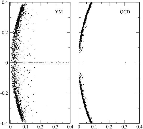
Figure 5: The low lying eigenvalue spectrum of the Dirac operator on 50 pure Yang-Mills (left) and 50 equilibrated dynamical (right) configurations. Both panels correspond to $8^{3}\times 24$, $a\approx 0.14\,$fm lattices with the same lattice quark masses.

VI Conclusion

In this paper we discussed the Partial Global Stochastic Update method and its use to simulate dynamical fixed point fermions. The original method is combined with several improvement techniques. By separating and controlling both the UV and IR modes of the Dirac operator and the fluctuations of its stochastic estimator we found the update efficient on moderate volumes even near the chiral limit. To illustrate the algorithm we presented some preliminary results on $8^{3}\times 24,$ $a\approx 0.14\,$fm lattices with 2+1 flavors with an approximately massless light doublet.