QED₃ on a space-time lattice: compact versus noncompact formulation

Abstract

We study quantum electrodynamics in a (2+1)-dimensional space-time with two flavors of dynamical fermions by numerical simulations on the lattice. We discretize the theory using both the compact and the noncompact formulations and analyze the behavior of the chiral condensate and of the monopole density in the finite lattice regime as well as in the continuum limit. By comparing the results obtained with the two approaches, we draw some conclusions about the possible equivalence of the two lattice formulations in the continuum limit.

I Introduction

Quantum electrodynamics in 2+1 dimensions (QED₃) is interesting as a toy model for investigating the mechanism of confinement in gauge theories Po , and as an effective description of low-dimensional, correlated, electronic condensed matter systems, like spin systems us ; senthil , or high-$T_{c}$ superconductors MaPa . While the compact formulation of QED₃ appears to be more suitable for studying the mechanism of confinement, both compact AM and noncompact formulations arise in condensed matter systems. Our paper aims to elucidate some aspects of the relationship between these two formulations of QED₃ on the lattice.

Polyakov showed that compact QED₃ without fermion degrees of freedom is always confining Po . Any pair of test electric charge and anti-charge is confined by a linear potential, as an effect of proliferation of instantons, which are magnetic monopole solutions in three dimensions. The plasma of such monopoles is what is responsible for confinement of electrically charged particles. If compact QED₃ is coupled to matter fields it has been argued deconf that the interaction between monopoles could turn from $1/x$ to $-\ln{(x)}$ at large distances $x$, so that the deconfined phase may become stable at low temperature. The issue of the existence of a confinement-deconfinement transition in QED₃ at $T=0$ is still controversial, as it has also been proposed that compact QED₃ with massless fermions is always in the confined phase HeSe ; AzLu ; also, in the limit of large flavor number, it has been argued that monopoles should not play any role in the confinement mechanism Herm . At finite temperature, parity invariant QED₃ coupled with fermionic matter undergoes a Berezinsky-Kosterlitz-Thouless transition to a deconfined phase griseso .

The issue of charge confinement in $2+1$ dimensional gauge models comes out to be relevant in the context of quantum phase transitions, as well. Indeed, recently it has been proposed that phenomena similar to deconfinement in high energy physics might appear in planar correlated systems, driven to a quantum (that is, zero-temperature) phase transition between an antiferromagnetically ordered (Neél) phase, and a phase with no order by continuous symmetry breaking us ; senthil . The most suitable candidate for a theoretical description of the system near the quantum critical point is a planar gauge theory, either with Fermionic matter us , or with Bosonic matter senthil .

At finite $T$ noncompact QED₃ comes about to be relevant in the analysis of the pseudo gap phase pseudo of cuprates. This phase arises from the fact that, upon doping the cuprate, a gap opens at some temperature $T^{\star}$ which is quite larger than the critical temperature $T_{C}$ for the onset of superconductivity. Both temperatures $T^{\star}$ and $T_{C}$ are doping dependent quantities and the gap is strongly dependent upon the direction in momentum space, since it exhibits $d$-wave symmetry TsuKi .

In Fig. 1 we report the phase diagram of high-$T_{c}$ cuprates. For small-$x$ phase is characterized HaTh by an insulating antiferromagnet (AF); by increasing $x$, this phase evolves into a spin density wave (SDW), that is a weak antiferromagnet. The pseudo gap phase is located between this phase and the $d$-wave superconducting (dSC) one.

The effective theory of the pseudo gap phase pseudo turns out to be QED₃ MaPa ; Fra ; Her , with spatial anisotropies in the covariant derivatives, that is with different values for the Fermi and the Gap velocities HaTh , and with Fermionic matter given by spin-$1/2$ chargeless excitations of the superconducting state (spinons). These excitations are minimally coupled to a massless gauge field, which arises from the fluctuating topological defects in the superconducting phase. The SDW order parameter is identified with the order parameter for chiral symmetry breaking (CSB) in the gauge theory, that is, $\langle\bar{\psi}\psi\rangle$ Her . There can be two possibilities; if $\langle\bar{\psi}\psi\rangle$ is different from zero, then the $d$-wave superconducting phase is connected to the spin density wave one (see Fig. 1 case b); otherwise the two phases are separated at $T=0$ by the pseudo gap phase (see Fig. 1 case a).

Confinement and chiral symmetry breaking go essentially together as strong coupling phenomena in gauge theories; while confinement is an observed property of the strong interactions and it is an unproven, but widely believed feature of non-abelian gauge theories in four space-time dimensions, chiral symmetry is only an approximate symmetry of particle physics, since the up and down quarks are light but not massless. Central to our understanding of CSB is the existence of a critical coupling: when fermions have a sufficiently strong attractive interaction there is a pairing instability and the ensuing condensate breaks some of the flavor symmetries, generate quark masses, and represents chiral symmetry in the Nambu-Goldstone mode namgot ; modernnamgot . The issue of a critical coupling has been widely investigated in 2+1 dimensional gauge theories cc1 ; cc2 ; cc3 . Typically, the dimensionless expansion parameter is $1/N_{f}$. Using the Schwinger-Dyson equations cc1 or a current algebra approach diaseso for QED₃ and QCD₃ one finds that there is a critical number of flavors, $N_{f,c}$, such that only for $N_{f}$ lesser than $N_{f,c}$ chiral symmetry is broken; for $N_{f}$ bigger than $N_{f,c}$ chirality is unbroken and quarks remain massless. For QED₃ this result has been the subject of some debate cc1 ; cc2 ; cc4 ; cc5 ; ApWi ; ApCoSc ; Fischer:2004nq ; there are, however, numerical simulations simulflav ; HaKoSt ; HaKoScSt of QED₃, which find an $N_{f,c}$ remarkably close to the results reported in Ref. cc1 .

Even if far from the scaling regime, strong coupling gauge theories on the lattice provide interesting clues on the issue of CSB. In fact, one can show that, in the strong coupling limit, a Hamiltonian with $N_{c}$ colors of fermions and $N_{f}/2$ lattice flavors of staggered fermions is effectively a $U(N_{f}/2)$ quantum antiferromagnet with representations determined by $N_{c}$ and $N_{f}$ strongcoupling . CSB is then associated strongcoupling either to the formation of a $U(1)$ commensurate charge density wave or of a $SU(N_{f}/2)$ spin density wave, i.e. to the formation of Neél order. Quantum antiferromagnets with the representations considered in Ref. strongcoupling have been analyzed in Ref. reasac where it was found that, for small enough $N_{f}$, the ground state is ordered. Also, when $N_{f}$ is increased there is a phase transition, for $N_{f}\sim N_{c}$, to a disordered state. In this picture, the large $N_{c}$ limit is the classical limit where Neél order is favored and the small $N_{c}$ and large $N_{f}$ limit are where fluctuations are large and disordered ground states are favored.

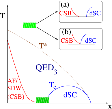
Figure 1: Phase diagram in the $(x,T)$ plane Fra ; here $x$ represents the doping and $T$ the temperature.

We shall not try to ascertain in this paper the critical number of flavours $N_{f,c}$. Here, we shall analyze the relationship between monopole density and fermion mass and compare the results obtained for the compact and noncompact lattice formulation of this gauge model. In particular, we revisit the analysis of Fiebig and Woloshyn of Refs. FiWo1 ; FiWo2 , where the dynamic equivalence between the two formulations of (isotropic) QED₃ is claimed to be valid in the finite lattice regime. In this paper we shall extend the comparison to the continuum limit, following the same approach as in Refs. FiWo1 ; FiWo2 : namely we shall analyze the behavior of the chiral condensate and of the monopole density as the continuum limit is reached.

In Section II we describe the model and its properties both in the continuum and on the lattice. Moreover, the method for detecting monopoles on the lattice is illustrated.

In Section III a description of both compact and noncompact formulations of QED₃ is given.

In Section IV we present our numerical result for the chiral condensate and the monopole density in the region in which the continuum limit is reached. Then, we compare our results with those of Fiebig and Woloshyn FiWo1 ; FiWo2 .

Section V is devoted to conclusions.

II The model and its properties

The continuum Lagrangian density describing QED₃ is given in Minkowski metric Ap by

$${\cal L}=-\frac{1}{4}F_{\mu\nu}^{2}+\overline{\psi}_{i}iD_{\mu}\gamma^{\mu}\psi_{i}-m_{0}\overline{\psi}_{i}\psi_{i}\;,$$ (1)

where $D_{\mu}=\partial_{\mu}-ieA_{\mu}$, $F_{\mu\nu}$ is the field strength and the fermions $\psi_{i}$ ($i=1,\dots,N_{f}$) are 4-component spinors. Since QED₃ is a super-renormalizable theory, dim$[e]=+1/2$, the coupling does not display any energy dependence. One may define three $4\times 4$ Dirac matrices

$$\gamma^{0}=\left(\begin{array}[]{cc}\sigma_{3}&0\\ 0&-\sigma_{3}\end{array}\right)\;,\hskip 28.45274pt\gamma^{1}=\left(\begin{array}[]{cc}i\sigma_{1}&0\\ 0&-i\sigma_{1}\end{array}\right)\;,$$

$$\gamma^{2}=\left(\begin{array}[]{cc}i\sigma_{2}&0\\ 0&-i\sigma_{2}\end{array}\right)\;,$$ (2)

and two more matrices anticommuting with them: namely

$$\gamma^{3}=i\left(\begin{array}[]{cc}0&1\\ 1&0\end{array}\right)\;,\hskip 28.45274pt\gamma^{5}=i\left(\begin{array}[]{cc}0&1\\ -1&0\end{array}\right)\;.$$ (3)

The massless theory will therefore be invariant under the chiral transformations

$$\psi\rightarrow e^{i\alpha\gamma^{3}}\psi\;,\qquad\psi\rightarrow e^{i\beta\gamma^{5}}\psi\;.$$ (4)

If one writes a 4-component spinor as $\psi=\left(\begin{array}[]{c}\psi_{1}\\ \psi_{2}\end{array}\right),$ the mass term becomes

$$m\overline{\psi}\psi=m\psi_{1}^{\dagger}\sigma_{3}\psi_{1}-m\psi_{2}^{\dagger}\sigma_{3}\psi_{2}\;.$$

Since in three dimensions the parity transformation reads

$$\psi_{1}(x_{0},x_{1},x_{2}) \rightarrow \sigma_{1}\psi_{2}(x_{0},-x_{1},x_{2})\;,$$

$$\psi_{2}(x_{0},x_{1},x_{2}) \rightarrow \sigma_{1}\psi_{1}(x_{0},-x_{1},x_{2})\;,$$ (5)

then $m\overline{\psi}\psi$ is parity conserving.

The lattice Euclidean action AlFaHaKoMo ; HaKoSt using staggered fermion fields $\overline{\chi},\chi$, is given by

$$S=S_{G}+\sum_{i=1}^{N}\sum_{n,m}\overline{\chi}_{i}(n)M_{n,m}\chi_{i}(m)\;,$$ (6)

where $S_{G}$ is the gauge field action and the fermion matrix is given by

$$M_{n,m}[U]$$ (7)

$$=\sum_{\nu=1,2,3}\frac{\eta_{\nu}(n)}{2}\left\{[U_{\nu}(n)]\delta_{m,n+\hat{\nu}}-[U_{\nu}^{\dagger}(m)]\delta_{m,n-\hat{\nu}}\right\}\;.$$

The action (6) allows to simulate $N=1,2$ flavours of staggered fermions corresponding to $N_{f}=2,4$ flavours of 4-component fermions $\psi$ BuBu . $S_{G}$ is different for the compact and noncompact formulation of QED₃.

For the compact formulation one has

$$S_{G}[U]=\beta\sum_{n,\mu<\nu}{\left[1-\frac{1}{2}\left(U_{\mu\nu}(n)+U_{\mu\nu}^{\dagger}(n)\right)\right]}\;,$$ (8)

where $U_{\mu\nu}(n)$ is the “plaquette variable” and $\beta=1/(e^{2}a)$, $a$ being the lattice spacing. Instead, in the noncompact formulation one has

$$S_{G}[\alpha]=\frac{\beta}{2}\sum_{n,\mu<\nu}F_{\mu\nu}(n)F_{\mu\nu}(n)\;,$$ (9)

where

$$F_{\mu\nu}(n)=\{\alpha_{\nu}(n+\hat{\mu})-\alpha_{\nu}(n)\}-\{\alpha_{\mu}(n+\hat{\nu})-\alpha_{\mu}(n)\}$$ (10)

and $\alpha_{\mu}(n)$ is the phase of the “link variable” $U_{\mu}(n)=e^{i\alpha_{\mu}(n)}$, related to gauge field by $\alpha_{\mu}(n)=aeA_{\mu}(n)$.

Monopoles are detected in the lattice using the method given by DeGrand and Toussaint DeTo : due to the Gauss’s law, the total magnetic flux emanating from a closed surface allows to determine if the surface encloses a monopole. The monopole density is defined by half of the total number of monopoles and antimonopoles divided by the number of elementary cubes in the lattice. We apply this definition for both the compact and the noncompact formulations of the theory, although some caution should be used in this respect. Indeed, monopoles are classical solutions of the theory with finite action only for compact QED₃, where they are known to play a relevant role. In the noncompact formulation of QED₃ they are not classical solutions, but they could give a contribution to the Feynman path integral owing to the periodic structure of the fermionic sector HaWe .

III Compact versus noncompact formulation

In order to investigate the onset of the continuum physics, it is convenient to consider a dimensionless observable and to evaluate it from the lattice for increasing $\beta$ until it reaches a plateau. Such an observable can be taken to be $\beta^{2}\langle\overline{\chi}\chi\rangle$, which is expected to become constant in the continuum ($\beta\rightarrow\infty$) limit simulflav ; DaKoKo2 . Numerical simulations show two regimes: for $\beta$ larger than a certain value, the theory is in the continuum limit (flat dependence of a dimensionless observable from $\beta$), otherwise the system is in a phase with finite lattice spacing. In the former regime, the theory describes continuum physics, in the latter one it is appropriate to describe a lattice condensed-matter-like system.

There are a couple of papers by Fiebig and Woloshyn in which the two formulations are compared in the finite lattice regime FiWo1 ; FiWo2 . In these papers the $\beta$-dependence of the chiral condensate and of the monopole density for lattice QED₃ with $N_{f}=0$ and $N_{f}=2$ are analyzed for both compact and noncompact formulations in the finite lattice regime.

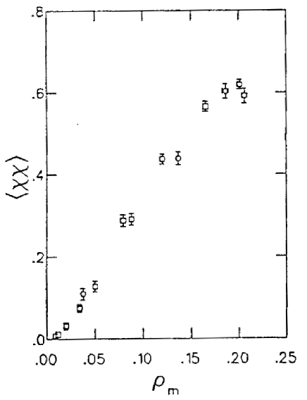
Figure 2: Correlation between $\langle\overline{\chi}\chi\rangle$ and $\rho_{m}$ for the compact (circles) and the noncompact (boxes) theories for $N_{f}=2$ and $8^{3}$ lattice according to Ref. FiWo2 .

It is shown there that, when $\langle\overline{\chi}\chi\rangle$ is plotted versus the monopole density $\rho_{m}$, data points for both theories fall on the same curve to a good approximation (see Fig. 2). This led the authors of Refs. FiWo1 ; FiWo2 to the conclusion that the physics of the chiral symmetry breaking is the same in the two theories.

Our program is to study if the conclusion reached by Fiebig and Woloshyn can be extended to the continuum limit, by looking at the same observables they considered: namely the chiral condensate and the monopole density.

IV Numerical results

Since QED₃ is a super-renormalizable theory, the coupling constant does not display any lattice space dependence. The continuum limit is approached by merely sending $\beta=1/(e^{2}a)$ to infinity. In this limit all physical quantities can be expressed in units of the scale set by the coupling $e$. Therefore, it is natural to work in terms of dimensionless variables such as $\beta m$, $L/\beta$ or $\beta^{2}\langle\overline{\chi}\chi\rangle$, which depend on $e$ ($L$ is the lattice size).

The signature that the continuum limit is approached is that data taken at different $\beta$ should overlap on a single curve when plotted in dimensionless units HaKoSt .

In practice, numerical results will not describe the correct physics of the system even in the continuum limit because of finite volume effects which are particularly significant in our case, due to the presence of a massless particle, the photon. In principle one should get rid of these effects by taking $L/\beta\rightarrow\infty$. In practice, this ratio is taken to be large, but finite. In Ref. GuRe the authors conclude that in order to find chiral symmetry breaking for $N_{f}=2$ at least a ratio $L/\beta\approx 5\times 10^{3}$ is required. In our simulations the largest value for the $L/\beta$ ratio has been 20.

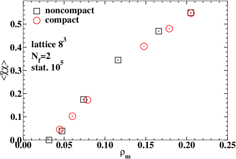
Figure 3: As in Fig. 2, according to our results.

Our Monte Carlo simulation code was based on the hybrid updating algorithm, with a microcanonical time step set to $dt=0.02$. We simulated one flavour of staggered fermions corresponding to two flavours of 4-component fermions. Most simulations were performed on a $12^{3}$ lattice, for bare quark mass ranging in the interval $am=0.01\div 0.05$. We made refreshments of the gauge (pseudofermion) fields every 7 (13) steps of the molecular dynamics. In order to reduce autocorrelation effects, “measurements” were taken every 50 steps. Data were analyzed by the jackknife method combined with binning.

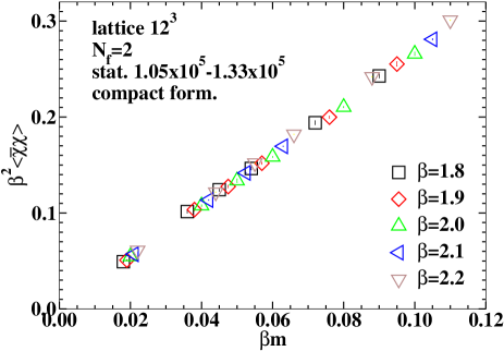
Figure 4: $\beta^{2}\langle\overline{\chi}\chi\rangle$ versus $\beta m$ in the compact formulation.

As a first step, we have reproduced the results by Fiebig and Woloshyn which are shown in Fig. 2. We find that also in our case data points from the two formulations nicely overlap (see Fig. 3). It should be noticed that data of Fig. 2 were obtained using a linear fit with two masses ($am$=0.025, 0.05) whilst those of Fig. 3 have been obtained by a quadratic fit with four masses ($am$=0.02, 0.03, 0.04, 0.05), nevertheless the conclusion is the same in both cases. We have verified that if we perform a linear fit on the subset of our data with masses $am$=0.02 and 0.05 and on the subset with masses $am$=0.03 and 0.05, our results nicely compare with those plotted in Fig. 2.

Then, in Fig. 4 we plot data for $\beta^{2}\langle\overline{\chi}\chi\rangle$ obtained in the compact formulation versus $\beta m$. We restrict our attention to the subset of $\beta$ values for which data points fall approximately on the same curve, which in the present case means $\beta=1.9,2.0,2.1$, corresponding to $L/\beta=6.31,6.00,5.71$. A linear fit of these data points gives $\chi^{2}$/d.o.f. $\simeq 8.4$ and the extrapolated value for $\beta m\rightarrow 0$ turns out to be $\beta^{2}\langle\overline{\chi}\chi\rangle=(1.54\pm 0.25)\times 10^{-3}$. Restricting the sample to the data at $\beta=2.1$, the $\chi^{2}/$d.o.f. lowers to $\simeq 1.3$ and the extrapolated value becomes $\beta^{2}\langle\overline{\chi}\chi\rangle=(0.94\pm 0.28)\times 10^{-3}$, thus showing that there is a strong instability in the determination of the chiral limit. If instead a quadratic fit is used for the points obtained with $\beta=1.9,2.0,2.1$, we get $\beta^{2}\langle\overline{\chi}\chi\rangle=(0.91\pm 0.45)\times 10^{-3}$ with $\chi^{2}$/d.o.f. $\simeq 8.7$. Owing to the large uncertainty, this determination turns out to be compatible with both the previous ones.

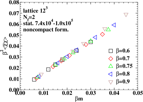
Figure 5: $\beta^{2}\langle\overline{\chi}\chi\rangle$ versus $\beta m$ in the noncompact formulation.

In Fig. 5 we plot data for $\beta^{2}\langle\overline{\chi}\chi\rangle$ obtained in the noncompact formulation versus $\beta m$. Following the same strategy outlined before, we restrict our analysis to the data obtained with $\beta=0.7,0.75,0.8$, which correspond to $L/\beta=17.14,16,15$.

If we consider a linear fit of these data and extrapolate to $\beta m\rightarrow 0$, we get $\beta^{2}\langle\overline{\chi}\chi\rangle=(0.45\pm 0.03)\times 10^{-3}$ with $\chi^{2}$/d.o.f. $\simeq 17$. Performing the fit only on the data obtained with $\beta=0.8$, for which a linear fit gives the best $\chi^{2}/$d.o.f. value $\simeq 16$, we obtain the extrapolated value $\beta^{2}\langle\overline{\chi}\chi\rangle=(0.66\pm 0.07)\times 10^{-3}$. Therefore, also in the noncompact formulation the chiral extrapolation resulting from a linear fit is largely unstable. A quadratic fit in this case gives instead a negative value for $\beta^{2}\langle\overline{\chi}\chi\rangle$.

The comparison of the extrapolated value for $\beta^{2}\langle\overline{\chi}\chi\rangle$ in the two formulations is difficult owing to the instabilities of the fits and to the low reliability of the linear fits, as suggested by the large values of the $\chi^{2}/$d.o.f. Taking an optimistic point of view, one could say that the extrapolated $\beta^{2}\langle\overline{\chi}\chi\rangle$ for $\beta=2.1$ in the compact formulation is compatible with the extrapolated value obtained in the noncompact formulation for $\beta=0.8$.

It is worth mentioning that our results in the noncompact formulation are consistent with known results: indeed, if we carry out a linear fit of the data for $\beta=0.6,0.7,0.8$ and $am$=0.02, 0.03, 0.04, 0.05 and extrapolate, we get $\beta^{2}\langle\overline{\chi}\chi\rangle=(1.30\pm 0.07)\times 10^{-3}$ with an admittedly large $\chi^{2}/$d.o.f. $\simeq 20$, but very much in agreement with the value $\beta^{2}\langle\overline{\chi}\chi\rangle=(1.40\pm 0.16)\times 10^{-3}$ obtained in Ref. AlFaHaKoMo .

We stress again that our results are plagued by strong finite volume effects, therefore our conclusions on the extrapolated values of $\beta^{2}\langle\overline{\chi}\chi\rangle$ are significant only in the compact versus noncompact comparison we are interested in. We do not even try to draw any conclusion from our data on the critical number of the flavours. As a matter of fact a recent paper HaKoSt shows that, if effects are carefully monitored and large lattices, up to $50^{3}$, are used, it is possible to establish that $\beta^{2}\langle\overline{\chi}\chi\rangle\leq 5\times 10^{-5}$. For the comparison between compact and noncompact QED₃ it is pertinent to carry out the numerical analysis with an (approximately) constant value of the ratio $L/\beta$. This condition is indeed verified even if we performed simulations on lattices with fixed ($L=12$) size, since the range of allowed values for $\beta$ corresponding to the continuum limit is narrow ($\beta=1.8\div 2.2$ in the compact case, $\beta=0.6\div 0.9$ in the noncompact case). Finite volume effects play a “second order” role in our work, since they probably only affect the extension of the continuum limit window of $\beta$ values.

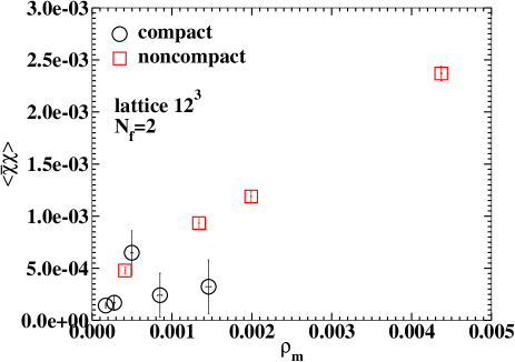
Figure 6: $\langle\overline{\chi}\chi\rangle$ versus $\rho_{m}$ in both the compact and the noncompact formulations on a $12^{3}$ lattice.

In Fig. 6 we plot $\langle\overline{\chi}\chi\rangle$ versus the monopole density $\rho_{m}$. Differently from Figs. 2-3, it is not evident with the present results that the two formulations are equivalent also in the continuum limit, although such an equivalence cannot yet be excluded.

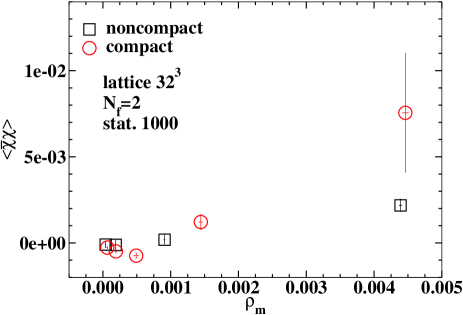
Figure 7: $\langle\overline{\chi}\chi\rangle$ versus $\rho_{m}$ in both the compact and the noncompact formulations on a $32^{3}$ lattice.

In Fig. 7 we plot again $\langle\overline{\chi}\chi\rangle$ versus the monopole density $\rho_{m}$, but now on a $32^{3}$ lattice. In this case the chiral condensate is extrapolated to zero mass by a quadratic fit. In spite of the negative value taken by $\langle\overline{\chi}\chi\rangle$ for large $\beta$, in this case data for both formulations seem to fall on the same curve.

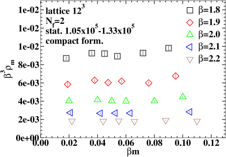
Figure 8: $\beta^{3}\rho_{m}$ versus $\beta m$ in the compact formulation.

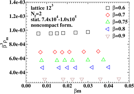
Figure 9: $\beta^{3}\rho_{m}$ versus $\beta m$ in the noncompact formulation.

In Fig. 8 and Fig. 9 we plot $\beta^{3}\rho_{m}$ versus $\beta m$ for the two formulations; the former quantity is dimensionless, therefore, in analogy with the previous cases, we expect that data at different $\beta$ values should fall on a single curve in the continuum limit. Our results show that this is not the case, this suggesting that the continuum limit has not been reached for the monopole density.

Simulations on the $32^{3}$ lattice give practically the same results for $\beta^{3}\rho_{m}$, indicating that this observable, unlike $\beta^{2}\langle\overline{\chi}\chi\rangle$, is volume independent.

It is important to observe, however, that the monopole density is independent of the fermion mass. Since the mechanism of confinement in the theory with infinitely massive fermions, i.e. in the pure gauge theory, is based on monopoles and since the monopole density is not affected by the fermion mass, we may conjecture that this same mechanism holds also in the chiral limit. This supports the arguments by Herbut about the confinement in the presence of massless fermion HeSe ; AzLu .

V Conclusions

In this paper we have compared the compact and the noncompact formulations of QED₃ by looking at the behavior of the chiral condensate and the monopole density.

Numerical results for $\beta^{2}\langle\overline{\chi}\chi\rangle$ are compatible with those obtained by other groups, although it is still questionable if the continuum limit has been reached and if the chiral limit is stable. The biggest difficulty for this observable is that the chiral extrapolation is rough when a linear fit is performed, but gives a negative value when instead a quadratic fit is considered. Massive calculations on larger lattices are needed to further reduce the finite volume effects and to stabilize the chiral limit.

As far as monopoles are concerned, they appear in smaller and smaller numbers for large $\beta$, this making the determination of the continuum limit for $\beta^{3}\rho_{m}$ rather problematic. Our results show, however, a very weak volume dependence.

We have analyzed also the relationship between the monopole density and the fermion mass, both in compact and noncompact QED₃. The weak dependence observed leads us to conclude that the Polyakov mechanism for confinement holds not only in the pure gauge theory, but also in presence of massless fermions.

Finally, we note that, although the chiral condensate and monopole density approach the continuum limit in two different ranges of $\beta$, the analysis à la “Fiebig and Woloshin” does not allow to exclude the equivalence of the compact and noncompact lattice formulations of QED₃.

References

- (1) A.M. Polyakov, Nucl. Phys. B 120, 429 (1977); Phys. Lett. B 59, 85 (1975).
- (2) B.A. Bernevig, D. Giuliano, R.B. Laughlin, Annals of Physics, 311, 182 (2004).
- (3) T. Senthil et al., Science 303, 1490 (2004).
- (4) N.E. Mavromatos, J. Papavassiliou, cond-mat/0311421 and references therein.
- (5) I. Affleck and J.B. Marston, Phys. Rev. B 37, 3774 (1988); Phys. Rev. B 39, 11538 (1989).
- (6) L.B. Ioffe and A.I. Larkin, Phys. Rev. B 39, 8988 (1989); J.B. Marston, Phys. Rev. Lett. 64, 1166 (1990); X.-G. Wen, Phys. Rev. B 65, 165113 (2002); H. Kleinert, F.S. Nogueira and A. Sudbo, Phys. Rev. Lett. 88, 232001 (2002); Nucl. Phys. B 666, 361 (2003).
- (7) I.F. Herbut and B.H. Seradjeh, Phys. Rev. Lett. 91, 171601 (2003).
- (8) V. Azcoiti, X.-Q. Luo, Mod. Phys. Lett. A 8, 3635 (1993).
- (9) M. Hermele, T. Senthil, M.P.A. Fisher, P.A. Lee, N. Nagaosa and X.-G. Wen, Phys. Rev. B 70, 214437 (2004).
- (10) G. Grignani, G.W. Semenoff, P. Sodano, Phys. Rev. D 53, 7157 (1996); Nucl. Phys. B473, 143 (1996).
- (11) T. Timusk and B. Statt, Rep. Prog. Phys. 62, 61 (1999).
- (12) C.C. Tsuei, J.R. Kirtley, Rev. Mod. Phys. 72, 969 (2000).
- (13) S. Hands, I.O. Thomas, hep-lat/0407029, hep-lat/0412009.
- (14) M. Franz and Z. Tesanovic, Phys. Rev. Lett. 87, 257003 (2001); Z. Tesanovic, O. Vafek and M. Franz, Phys. Rev. B 65, 180511 (2002); M. Franz, Z. Tesanovic, O. Vafek, Phys. Rev. B 66, 054535 (2002).
- (15) I.F. Herbut, Phys. Rev. B 66, 094504 (2002).
- (16) Y. Nambu, G. Jona-Lasinio, Phys. Rev. 122, 345 (1961).
- (17) V. Miransky, Nuovo Cimento Soc. Ital. Fis. 90A, 149 (1985); W.A. Bardeen, C.N. Leung, S. Love, Phys. Rev. Lett. 56, 1230 (1986); K. Yamawaki, M. Bando, K. Matumoto, Phys. Rev. Lett. 56, 1335 (1986); T. Appelquist, L.C.R. Wijewardhana, Phys. Rev. D 36, 568 (1987); R. Holdom, Phys. Rev. Lett. 60, 1233 (1988); W. Bardeen, C.N. Leung, S. Love, Nucl. Phys. B323, 493 (1989).
- (18) T. Appelquist, D. Nash, L.C. Wijewardana, Phys. Rev. Lett. 60, 2575 (1988); D. Nash, Phys. Rev. Lett. 62, 3024 (1989); T. Appelquist, D. Nash, Phys. Rev. Lett. 64, 721 (1990).
- (19) R. Pisarsky, Phys. Rev. D 44, 1866 (1991).
- (20) M.R. Pennington, D. Walsh, Phys. Lett. B 253, 246 (1991); D.C. Curtis, M.R. Pennington, D. Walsh, Phys. Lett. B 295, 313 (1992).
- (21) M.C. Diamantini, G.W. Semenoff, P. Sodano, Phys. Rev. Lett. 70, 3848 (1993).
- (22) P.W. Johnson, Argonne Workshop on Non-Perturbative QCD (unpublished).
- (23) D. Atkinson, P.W. Johnson, P. Maris, Phys. Rev. D 42, 602 (1990).
- (24) T. Appelquist, L.C.R. Wijewardhana, hep-ph/0403250.
- (25) T. Appelquist, A.G. Cohen, M. Schmaltz, Phys. Rev. D 60, 045003 (1999).
- (26) C. S. Fischer, R. Alkofer, T. Dahm and P. Maris, Phys. Rev. D 70 (2004) 073007.
- (27) E. Dagotto, J. Kogut, A. Kocic, Phys. Rev. Lett. 62, 1083 (1989); J. Kogut, J.-F. Lagae, Nucl. Phys. B (Proc. Suppl.), 30, 737 (1993).
- (28) S.J. Hands, J.B. Kogut, C.G. Strouthos, Nucl. Phys. B 645, 321 (2002).
- (29) S.J. Hands, J.B. Kogut, L. Scorzato and C.G. Strouthos, Phys. Rev. B 70, 104501 (2004).
- (30) G.W. Semenoff, Mod. Phys. Lett. A 7, 2811 (1992); M.C. Diamantini, E. Langmann, G.W. Semenoff, P. Sodano, in Field Theory of Collective Phenomena, pg. 411, World Scientific Publishing, Singapore, (1995), ISBN 981-02-1279-8; M.C. Diamantini, E. Langmann, G.W. Semenoff, P. Sodano, Nucl. Phys. B406, 595 (1993).
- (31) N. Read, S. Sachdev Phys. Rev. Lett. 62, 1694 (1989); Phys. Rev. B 42, 4568 (1990); Nucl. Phys. B 316, 609 (1990).
- (32) H.R. Fiebig and R.M. Woloshyn, Phys. Rev. D 42, 3520 (1990).
- (33) H.R. Fiebig and R.M. Woloshyn, Nucl. Phys. Proc. Suppl. 20, 655 (1991).
- (34) T.W. Appelquist et al., Phys. Rev. D 33, 3704 (1986).
- (35) J. Alexandre, K. Farakos, S.J. Hands, G. Koutsoumbas and S.E. Morrison, Phys. Rev. D 64, 034502 (2001).
- (36) C. Burden and A.N. Burkitt, Europhys. Lett. 3, 545 (1987).
- (37) T.A. DeGrand and D. Toussaint, Phys. Rev. D 22, 2478 (1980).
- (38) S. Hands, R. Wensley, Phys. Rev. Lett. 63, 2169 (1989).
- (39) E. Dagotto, A. Kocic, J.B. Kogut, Nucl. Phys. B 334, 279 (1990).
- (40) V.P. Gusynin, M. Reenders, Phys. Rev. D 68, 025017 (2003).