Investigations in 1+1 dimensional lattice $\phi^{4}$ theory

Abstract

In this work we perform a detailed numerical analysis of (1+1) dimensional lattice $\phi^{4}$ theory. We explore the phase diagram of the theory with two different parameterizations. We find that symmetry breaking occurs only with a negative mass-squared term in the Hamiltonian. The renormalized mass $m_{R}$ and the field renormalization constant $Z$ are calculated from both coordinate space and momentum space propagators in the broken symmetry phase. The critical coupling for the phase transition and the critical exponents associated with $m_{R}$, $Z$ and the order parameter are extracted using a finite size scaling analysis of the data for several volumes. The scaling behavior of $Z$ has the interesting consequence that $\langle\phi_{R}\rangle$ does not scale in $1+1$ dimensions. We also calculate the renormalized coupling constant $\lambda_{R}$ in the broken symmetry phase. The ratio $\lambda_{R}/m_{R}^{2}$ does not scale and appears to reach a value independent of the bare parameters in the critical region in the infinite volume limit.

I Introduction

Over the years the $1+1$ dimensional $\phi^{4}$ theories have been used and investigated for many purposes, including theoretical and algorithmic developments in novel nonperturbative approaches. There is a large body of work that deals with the theory in the continuum starting from the mid-seventies till now cphi . They involve techniques such as Hartree approximation, Gaussian effective potential, post Gaussian approximations, random phase approximation and discrete and continuum light front Hamiltonian. These studies have been done with a positive bare mass-squared ($m^{2}>0$) and diverging contribution to the mass at the lowest non-trivial order of the coupling ($O(\lambda)$) arising from normal ordering was cancelled by a counter term, effectively dropping the divergent piece. A phase transition to broken symmetry phase was found at strong quartic coupling. Critical value for $\lambda/m^{2}$ has been found to lie somewhere between 30 and 60.

Lattice regularization is naturally suited to determine the phase diagram of a quantum field theory. There has been an attempt on the lattice lw to extract the critical value of $\lambda/m^{2}$. This calculation was performed with a negative bare mass-squared term in the lattice action resulting in the broken symmetry phase at small coupling. The negative mass-squared was converted to a positive mass-squared in the infinite volume limit by a renormalization performed after the lattice data had been extracted and a critical value for $\lambda/m^{2}$ was quoted.

In this paper we investigate the 1+1 dimensional $\phi^{4}$ theory on the lattice. To the best of our knowledge, there does not exist any detailed study of the critical region of this theory using the nonperturbative numerical program of quantum field theories on the lattice. Our aim is to explicitly determine the scaling behavior of the renormalized mass, the renormalized coupling and the field renormalization constant including their amplitudes. We also want to investigate the topological sector of this theory in the broken phase. In a companion work tcphi we have calculated the topological charge using the same nonperturbative techniques and have shown its relation to the renormalized parameters in the quantum theory.

In this theory the quartic coupling has the dimension of mass-squared and a ‘physical’ (relevant in the continuum) quantity to calculate is the dimensionless ratio of the renormalized parameters $\lambda_{R}/m_{R}^{2}$. We determine the phase diagram in the two dimensional bare parameter space which agrees with the phase diagram of lw . We have not found a phase transition from the symmetric phase to the broken symmetry phase with a positive mass-squared term in the action. The symmetry breaking occurs in our lattice theory only with a negative mass-squared term. We perform a detailed study of the scaling region of the broken symmetry phase and determine the ratio $\lambda_{R}/m_{R}^{2}$ which appears to be constant in the scaling region irrespective of the bare lattice parameters. The vacuum expectation value of the renormalized field $\langle\phi_{R}\rangle$ also seems to be constant irrespective of the parameters in the scaling region of the $1+1$ dimensional theory. We have determined these ratios using numerical lattice techniques on a variety of lattice sizes. We have estimates for their infinite volume values.

For a nonperturbative approach like the lattice, the notion of perturbative renormalizability is to be replaced by existence of critical manifolds and universality classes. The $\phi^{4}$ theories are generally believed to be in the same universality class as the Ising model. This notion originally came from the Renormalization Group and in two Euclidean dimensions is consistent with a conjecture based on conformal field theory az . In our investigation we determine the critical exponents of $\langle\phi\rangle$ and $m_{R}$ independently in $\phi^{4}$ theory and find them to be the same as the Ising values. Another important ingredient relevant in our analysis is the field renormalization constant $Z$ which appears in the two point correlation function. The critical exponent of $Z$ emerging from our FSS analysis in $\phi^{4}$ theory is found to be consistent with the exponent of susceptibility in the Ising model.

Although it is not the ultimate goal of our work, our results provide an independent confirmation of the universality of Ising model and $\phi^{4}$ theory (with negative mass-squared) in 1+1 dimensions using numerical techniques of lattice field theory. However, in an actual calculation, always done in a bare theory with an ultraviolet cut-off like the lattice (which also has a finite size), there are many important issues still to be resolved, for example, the onset of the scaling region, effects of the finite size, possible scaling violation etc. The above needs to be done in each theory for a complete understanding of the process of the continuum limit.

In order to determine the ratio $\lambda_{R}/m_{R}^{2}$, we need to know the field renormalization constant $Z$ and the renormalized mass $m_{R}$ which can be defined and determined in two ways: 1) the exponential fall-off in Euclidean time of the zero-spatial-momentum bare lattice propagators in the coordinate space, and 2) the behavior of the momentum space propagators for small four-momenta. We expect respective critical exponents corresponding to the renormalized mass and the field renormalization constant to agree for the two methods and we verify this in the current paper. In this connection, we wish to point out that we have made use of finite size scaling for accurate determination of the critical point and verification and determination of the critical exponents. For recent calculations in 3+1 dimensional Ising model, see bdwnw .

Cluster algorithms, known for beating critical slowing down in Ising models, are not directly applicable to the $\phi^{4}$ theories. However, owing to a development by Wolff wolff2 using embedded Ising variables bt we have been able to use cluster algorithms in conjunction with the usual Metropolis Monte Carlo.

The plan of the paper is as follows. In Sec. II we define the two parameterizations of the $\phi^{4}$ theory on the lattice followed by section III where we discuss the use of embedded Ising variables in $\phi^{4}$ theory for use of the cluster algorithms. We show the phase structure of the lattice theory in section IV. In section V we present the calculation of the connected scalar propagator in coordinate space and momentum space and then in section VI we extract the critical exponents for mass $m_{R}$ and field renormalization constant $Z$ and determine the critical coupling using finite size scaling analysis. In Sec. VII the renormalized coupling constant $\lambda_{R}$ and the quantities $\lambda_{R}/m_{R}^{2}$ and $\phi_{R}$ are discussed. Finally in Sec. VIII we conclude with a summary of our results.

II $\phi^{4}$ theory on lattice

In this section we present the lattice action of (1+1) dimensional lattice $\phi^{4}$ theory in two different parameterizations.

II.1 Parameterization as in the Continuum

We start with the Lagrangian density in Minkowski space (in usual notations)

$${\cal L}=\frac{1}{2}\partial_{\mu}\phi\partial^{\mu}\phi-\frac{1}{2}m^{2}\phi^{2}-\frac{\lambda}{4!}\phi^{4}$$ (1)

which leads to the Lagrangian density in Euclidean space

$${\cal L}_{E}=\frac{1}{2}\partial_{\mu}\phi\partial_{\mu}\phi+\frac{1}{2}m^{2}\phi^{2}+\frac{\lambda}{4!}\phi^{4}.$$ (2)

Note that in one space and one time dimensions, the scalar field $\phi$ is dimensionless and the quartic coupling $\lambda$ has dimension of mass².

The Euclidean action is

$$S_{E}=\int d^{2}x{\cal L}_{E}.$$ (3)

Next we put the system on a lattice of spacing $a$ with

$$\int d^{2}x=a^{2}~{}\sum_{x}.$$ (4)

Because of the periodicity of the lattice sites in a toroidal lattice, the surface terms will cancel among themselves (irrespective of the boundary conditions on fields) enabling us to write

$$(\partial_{\mu}\phi)^{2}=-\phi\partial_{\mu}^{2}\phi$$ (5)

and on the lattice

$$\partial_{\mu}^{2}\phi=\frac{1}{a^{2}}\left[\phi_{x+\mu}+\phi_{x-\mu}-2\phi_{x}\right]~{}.$$ (6)

$\phi_{x\pm\mu}$ is the field at the neighboring sites in the $\pm\mu$ direction. Introducing dimensionless lattice parameters $m_{0}^{2}$ and $\lambda_{0}$ by $m_{0}^{2}=m^{2}~{}a^{2}$ and $\lambda_{0}=\lambda~{}a^{2}$ we arrive at the lattice action in two Euclidean dimensions

$$S=-\sum_{x}\sum_{\mu}\phi_{x}\phi_{x+\mu}~{}+~{}(2+\frac{m_{0}^{2}}{2})~{}\sum_{x}~{}\phi_{x}^{2}+\frac{\lambda_{0}}{4!}~{}\sum_{x}~{}\phi_{x}^{4}~{}.$$ (7)

We shall henceforth call this lattice action the continuum parameterization.

All dimensionful quantities in the following are expressed naturally in the lattice units, basically meaning that they become dimensionless in the lattice formulation by getting multiplied by appropriate powers of the lattice spacing $a$.

II.2 Another Parameterization

A different parameterization in terms of field $\Phi$ and parameters $\kappa$ and $\tilde{\lambda}$, henceforth called the lattice parameterization is obtained by setting

$$\phi=\sqrt{2\kappa}~{}\Phi,~{}~{}m_{0}^{2}=\frac{1-2\tilde{\lambda}}{\kappa}-2d,~{}~{}\lambda_{0}=6\frac{\tilde{\lambda}}{\kappa^{2}}$$ (8)

where, $d=2$ in our case. This leads to the lattice action

$$S^{\prime}=-2\kappa~{}\sum_{x}\sum_{\mu}\Phi_{x}\Phi_{x+\mu}~{}+~{}\sum_{x}\Phi_{x}^{2}~{}+~{}\tilde{\lambda}~{}\sum_{x}(\Phi_{x}^{2}-1)^{2}$$ (9)

where we have ignored an irrelevant constant.

In the limit $\tilde{\lambda}\rightarrow\infty$, configurations with $\Phi^{2}_{x}\neq 1$ are suppressed. As a result, field variables assume only two values $\Phi_{x}\rightarrow\pm 1$ and $S^{\prime}$ is reduced to the Ising action $S_{\rm Ising}$ with

$$S_{\rm Ising}=-2\kappa~{}\sum_{x}\sum_{\mu}\Phi_{x}\Phi_{x+\mu}.$$ (10)

The lattice action given in Eq. (9) is invariant under the staggered transformation

$$\kappa\rightarrow-\kappa,~{}~{}~{}~{}\Phi_{x}\rightarrow\Phi_{{\rm st},x}$$ (11)

where $\Phi_{{\rm st},x}=(-1)^{x_{1}+x_{2}}~{}\Phi_{x}$. As a result, if $\kappa_{c}$ is a critical point, there exists another critical point at $-\kappa_{c}$. We have three phases: broken phase for $\kappa>\kappa_{c}~{}\left(\langle\Phi\rangle\neq 0,~{}\langle\Phi_{\rm st}\rangle=0\right)$, symmetric phase for $-\kappa_{c}<\kappa<\kappa_{c}~{}\left(~{}\langle\Phi\rangle~{}=~{}\langle\Phi_{\rm st}\rangle=0\right)$ and a staggered broken phase for $\kappa<-\kappa_{c}~{}\left(~{}\langle\Phi\rangle=0,~{}\langle\Phi_{\rm st}\rangle\neq 0\right)$. Note that the staggered broken phase is inaccessible in the continuum parameterization.

Wherever possible, we have made use of the lattice parameterization to check the implementation of the our algorithm since it allows a cross checking of the critical points.

III Algorithm for updating configurations

It is well known that most algorithms become extremely inefficient near criticality (i.e near the continuum limit). This phenomenon is known as critical slowing down (CSD). To beat CSD in our $\phi^{4}$ theory (which has an embedded Ising variable as explained below) we have used a cluster algorithm (known to beat CSD in Ising-like systems) to update the embedded Ising variables and combined it with the usual Metropolis Monte Carlo algorithm. The variant of the cluster algorithm that we have used is due to Wolff wolff and is known as ‘single cluster algorithm’.

To see what an embedded Ising variable is and how it is made use of, note that the part of the $\phi^{4}$ action that responds to a change of sign is

$$S^{I}[\phi] = -\sum_{x,\mu}\phi_{x}\phi_{x+\mu}$$ (12)

$$= -\sum_{x,\mu}|\phi_{x}||\phi_{x+\mu}|\sigma_{x}\sigma_{x+\mu}$$

$$= -\sum_{x,\mu}J_{x,x+\mu}\sigma_{x}\sigma_{x+\mu}$$

where $\sigma_{x}={\rm sign}(\phi_{x})$ is called the embedded Ising variable and $J_{x,x+\mu}=|\phi_{x}||\phi_{x+\mu}|$ resembles a coupling that depends on both position and direction.

Notwithstanding the resemblance, the above action does not describe an inhomogeneous, anisotropic Ising model since the couplings $J$ will vary over configurations. In general one cannot update different aspects of a degree of freedom ( for example the modulus and sign of $\phi$) separately and independently. Nevertheless, updating the Ising sector (sign of $\phi$) in $\phi^{4}$ theory is legitimate owing to a result due to Wolff wolff2 that we will call Wolff’s theorem.

We describe the theory underlying this procedure, not always easy to find elsewhere. We start by explaining Wolff’s theorem .

Consider a group $G$ of transformations $T$ acting on the configurations $C$ of some system:

$$C\rightarrow TC.$$ (13)

Now let us consider the group G as an auxiliary statistical system whose (micro)states are the group elements {T}. We define the induced Hamiltonian governing the distribution of the auxiliary system by $H(TC)$ where $H$ is just the Hamiltonian of the original system now considered as a function of $T$.

Let us now define an algorithm W with transition probabilities $p(C;T\rightarrow T^{\prime})$ such that
1) $\sum_{T}e^{-H(TC)}p(C;T\rightarrow T^{\prime})=e^{-H(T^{\prime}C)}$,
2) $p(TC;T_{1}\rightarrow T_{2})=p(C;T_{1}T\rightarrow T_{2}T)$.

Wolff’s theorem states that a legitimate algorithm for updating the original system is
$\bullet$ Fix $C=C_{1}$ and $T=I$ (identity transformation),
$\bullet$ Update $T_{1}\rightarrow T_{2}$ using the W algorithm,
$\bullet$ Assign $C_{2}=T_{2}C_{1}$ as the new configuration.

We shall now demonstrate that if Wolff’s theorem is applied to $\phi^{4}$ theory with an appropriate choice of G, it is equivalent to updating the Ising sector independently.

Take $G=Z_{2}^{N}$ where N is the number of sites. Elements $T$ of $Z_{2}^{N}$ can be represented by Ising variables. $T=\{\sigma_{x}\}$ with $\sigma_{x}=+1$ or $-1$ so that

$$TC\equiv T\{\phi_{x}\}=\{\sigma_{x}\phi_{x}\}.$$ (14)

The induced Hamiltonian is

$$H(TC) = -\sum_{x,\mu}[\sigma_{x}\phi_{x}][\sigma_{x+\mu}\phi_{x+\mu}]$$

$$= -\sum_{x\mu}|\phi_{x}||\phi_{x+\mu}|\sigma_{x}s_{x}\sigma_{x+\mu}s_{x+\mu}$$

$$= -\sum_{x,\mu}|\phi_{x}||\phi_{x+\mu}|s_{x}^{\prime}s_{x+\mu}^{\prime}$$

where $\phi_{x}=|\phi_{x}|s_{x}$ and $s_{x}^{\prime}=\sigma_{x}s_{x}$.

The proof of our proposition follows if we note that the above Hamiltonian is indeed an inhomogeneous, anisotropic Ising Hamiltonian and there is a 1-1 mapping between the variables $s_{x}^{\prime}$ and $\sigma_{x}$.

We have used Wolff’s single cluster variant of the cluster algorithm to update the Ising variables. Since the configuration space for the $\phi^{\prime}s$ is much larger than that for the Ising variables, to ensure ergodicity, the algorithm was blended with the standard Metropolis algorithm. The blending ratio used was 1:1 i.e every cluster sweep was followed up by a Metropolis sweep.

We summarize the main steps in the algorithm. We start with some initial configuration for the $\phi$ fields. We then update the sign of the $\phi$ fields using Wolff‘s single cluster algorithm using the action (12): We choose some site (seed) at random and select a group of $\phi$ fields (cluster) around the seed having the same sign as the field sitting at the seed. The probability for selecting a particular field is governed by the action (12). This process is called growing a cluster. We flip the sign of the fields belonging to the cluster (the variables $\sigma$ in (12)) when the cluster is fully grown. Finally we execute a Metropolis sweep over the entire lattice updating the full $\phi$ fields. This completes one updation cycle.

Throughout this paper we have used periodic boundary conditions. However, in the companion work tcphi dealing with topological charge we have used antiperiodic boundary conditions where cluster algorithms do not work hasen .

IV Phase Structure

The phase structure is determined by looking at the order parameter $\langle\phi\rangle$ which takes a nonzero value in the spontaneously broken phase. With the cluster algorithm however, since the sign of the field of all the members of the cluster are flipped in every updation cycle the algorithm actually enforces tunneling between the two degenerate vacua in the broken phase. As a result, as an artifact, the average of $\phi$ over configurations, i.e., the expectation value becomes zero. Thus to get the correct nonzero value for the condensate we measure $\langle|\phi|\rangle$ where $\phi=\frac{1}{\rm Volume}\sum\limits_{\rm sites}\phi_{x}$. To understand the mod let us consider a local order parameter $\langle\phi_{x}\rangle$. Since the configurations will be selected at random dominantly from the neighborhood of either vacua in the broken phase, $\langle\phi_{x}\rangle$ will vanish when averaged over configurations thus wiping out the signature of a broken phase. If one uses $\langle|\phi_{x}|\rangle$ as the order parameter then in the broken phase it correctly projects itself onto one of the vacua yielding the appropriate non-zero value. The use of this mod, unfortunately, destroys the signal in the symmetric phase completely by wiping out the significant fluctuations in sign. However if we choose to use $\langle|\frac{1}{\rm Volume}\sum\limits_{\rm sites}\phi_{x}|\rangle$, it correctly captures the broken phase as well as the symmetric phase. While the sign fluctuation over configurations are still masked, the fluctuations over sites survive producing $\langle|\phi|\rangle=0$ correctly in the symmetric phase.

The phase diagram for the continuum parameterization obtained for a $512^{2}$ lattice is presented in Fig. 1. Classically, spontaneous symmetry breaking (SSB) occurs for negative $m_{0}^{2}$. For small negative $m_{0}^{2}$, as two minima are shallow and very close to each other, quantum fluctuations can restore the symmetry. So, larger negative values of $m_{0}^{2}$ are required for SSB to take place. Consequently, the phase transition line is found in the negative $m_{0}^{2}$ semiplane. Our phase diagram agrees qualitatively with that obtained for much smaller lattices in ct ; aw . In lw the authors have extrapolated their results to infinite volume. We find that our $512^{2}$ lattice results are as good as the infinite volume result in lw .

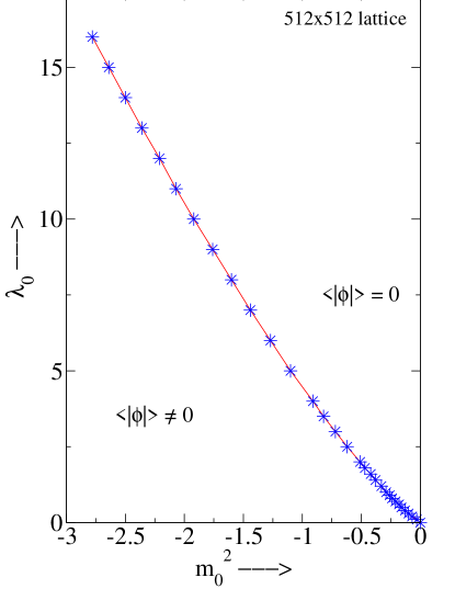
Figure 1: Phase diagram for continuum parameterization

In lattice parameterization, phase diagram obtained for a $100^{2}$ lattice is presented in Fig. 2(a). We have restricted ourselves only to $\kappa\geq 0$ region. The symmetry of the phase diagram for $\kappa<0$ and $\kappa>0$ is evident from the behavior of $\langle\Phi\rangle$ and $\langle\Phi_{\rm st}\rangle$ as a function of $\kappa$, shown in Fig. 2(b).

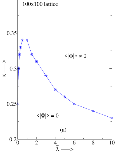
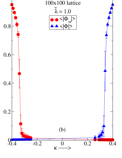
Figure 2: (a) Phase diagram for lattice parameterization. (b) Manifestation of the staggered symmetry of lattice parameterization of the action.

As mentioned in the Introduction, in the continuum version of $1+1$ dimensional $\phi^{4}$ theory with a positive mass-squared term in the Hamiltonian, there have been many attempts to calculate critical couplings for phase transition from the symmetric phase to the broken phase cphi . We have investigated the phase diagram of the lattice theory in the region of positive mass-squared and have been unable to detect a phase transition in this region of the parameter space. In Fig. 3 we show the measurement of the mass gap $m_{R}$ extracted from coordinate space propagator in positive mass-squared region. We find that the mass gap $m_{R}$ monotonically increases with the coupling.

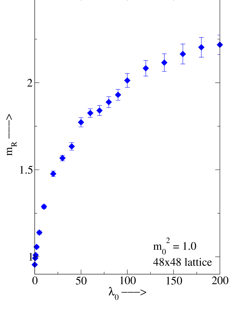
Figure 3: Mass gap for $+$ ve $m_{0}^{2}$.

An alternative way to probe the same region of the parameter space of the continuum parameterization is to perform simulations with the lattice parameterization of the action. From the phase diagram for the latter presented in Fig. 2(a), we reconfirm the absence of phase transition for the lattice theory in the positive mass-squared region in the continuum parameterization since this whole region can be mapped onto the symmetric phase in the lattice parameterization using the transformation Eq. (8).

V Calculation of Propagator

We have made use of two-point connected correlation function to calculate the fundamental boson mass and field renormalization constant. We have carried out our simulation both in coordinate and momentum space.

V.1 Coordinate space

In coordinate space, 2-point connected correlation function $G_{c}\left(x,x_{0}\right)$ is given by

$$G_{c}(x,x_{0}) = \left<\phi\left(\vec{x},t\right)\phi\left(\vec{x_{0}},t_{0}\right)\right>-\left<\phi\left(\vec{x},t\right)\right>\left<\phi\left(\vec{x_{0}},t_{0}\right)\right>$$ (16)

$$= \left<\phi\left(\vec{x},t\right)\phi\left(\vec{x_{0}},t_{0}\right)\right>-\left<\phi\right>^{2}.$$

For the derivation of the last equation translational invariance has been assumed. As explained before, we actually calculate $\left<|\phi|\right>$ instead of $\left<\phi\right>$ in Eq. (16) The notation $\vec{x}$ may be confusing in 1+1 dimensions; however, it is kept to distinguish between the spatial and temporal directions.

We have extracted the renormalized scalar mass $m_{R}$ (pole mass) and the field renormalization constant $Z$ from

$$G_{c}\left(t\right)=\frac{Z}{2m_{R}}\left[e^{-m_{R}t}+e^{-m_{R}\left(L-t\right)}\right]+{\rm{~{}higher~{}states}}.$$ (17)

where $G_{c}\left(t\right)$ is the zero spatial momentum projection of the 2-point connected correlation function. The second exponential term in the RHS of the above equation is due to the periodicity of the lattice.

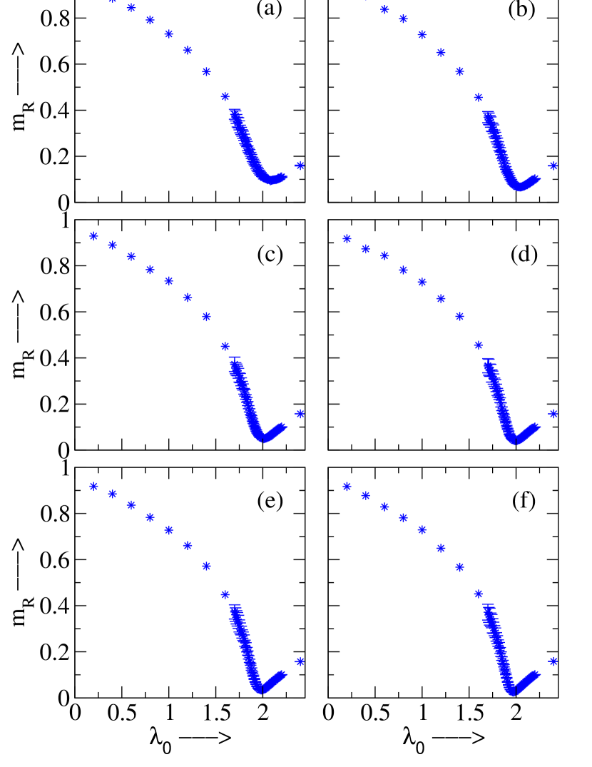
Figure 4: $m_{R}$ from coordinate space propagator for different lattices (a) $32^{2}$, (b) $48^{2}$, (c) $64^{2}$, (d) $80^{2}$, (e) $96^{2}$ and (f) $128^{2}$ ($m_{0}^{2}=-0.5$)

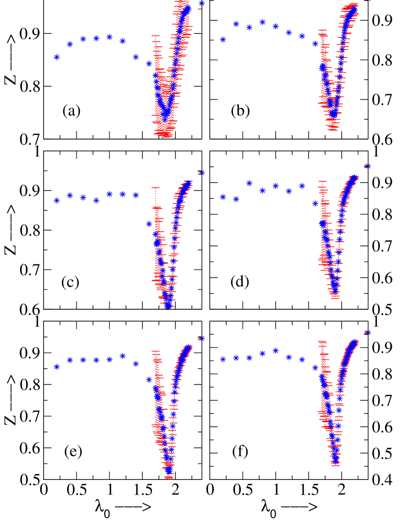
Figure 5: $Z$ from coordinate space propagator for different lattices (a) $32^{2}$, (b) $48^{2}$, (c) $64^{2}$, (d) $80^{2}$, (e) $96^{2}$ and (f) $128^{2}$ ($m_{0}^{2}=-0.5$)

In this calculation, to ensure thermalization, we have discarded the first $10^{6}$ configurations before starting our measurements. Measurements were carried out on $100$ bins of $2\times 10^{5}$ configurations. In each bin, to fulfill the requirement that measurements be made on statistically independent configurations, measurements were performed every tenth configuration (hop-length).

Figs. 5 and 5 show $m_{R}$ and $Z$ extracted from the connected propagator in coordinate space for lattices of six different sizes as function of $\lambda_{0}$ for fixed $m_{0}^{2}=-0.5$. The figures clearly demonstrate scaling of $m_{R}$ and $Z$ as one moves towards the critical point. The critical point is given roughly by the dip in each curve. These dips are clearly not at the same place for $m_{R}$ and $Z$ at the smaller lattices. A phenomenological finite size scaling analysis has been done in the next section on these data and the data obtained from momentum space propagators to calculate the critical exponents and the critical coupling in the infinite volume limit. Around the critical region in Figs. 5 and 5, all the curves have a thick appearance because of the proximity of the many data points with the associated errors shown for each point. Outside the scaling region, a region not of interest to us, the data is relatively sparse and we also have suppressed the error bars for them. Unlike in the Ising model ($\lambda_{0}\rightarrow\infty$), at finite $\lambda_{0}$ the $\langle|\phi|\rangle$ takes on large values outside the scaling region in the broken phase. In calculating the connected propagator, one performs a subtraction between the large expectation values of two quantities measured independently. This enhances the error bars outside the scaling region in the broken symmetry phase.

V.2 Momentum space

Connected propagator in momentum space is

$$G_{c}(p)=\sum_{x}e^{ipx}\left[\left<\phi_{x}\phi_{0}\right>-\left<\phi_{x}\right>\left<\phi_{0}\right>\right].$$ (18)

To improve statistics in numerical simulation, averaging over source $y$ is performed.

$$G\left(p\right) = \frac{1}{V}\sum_{x,y}e^{ip\left(x-y\right)}\left[\left<\phi_{x}\phi_{y}\right>-\left<\phi_{x}\right>\left<\phi_{y}\right>\right]$$ (19)

$$= \left<\frac{1}{V}\sum_{x,y}\phi_{x}\phi_{y}\cos p\left(x-y\right)\right>-\left|\left<\phi\right>\right|^{2}\delta\left(p\right).$$

At small momenta, the momentum space propagator behaves as

$$G\left(p\right)=\frac{Z^{\prime}}{m_{R^{\prime}}^{2}+{\hat{p}}^{2}}$$ (20)

where, ${\hat{p}}^{2}=4\sum\limits_{\mu}\sin^{2}\left(\frac{p_{\mu}}{2}\right)$ with $\mu=1,2$ is the dimensionless lattice equivalent of the momentum square in the continuum.

From the intercept of inverse propagator on the ordinate and slope at $\hat{p}^{2}=0$, $m_{R^{\prime}}$ and $Z^{\prime}$ can be determined. However it is only near the critical coupling that the pole of the propagator is actually near zero and it is here that $m_{R^{\prime}}$ approaches the pole mass $m_{R}$. A similar argument applies to $Z^{\prime}$ and $Z$. We have thus calculated the momentum space propagators only near the critical point.

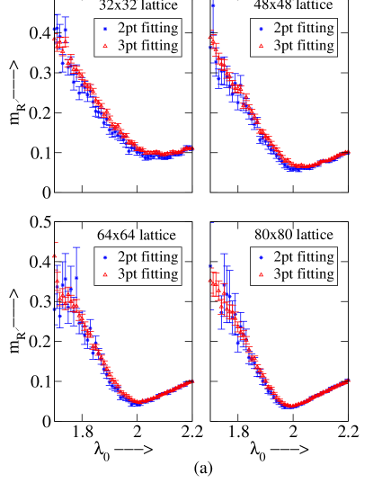
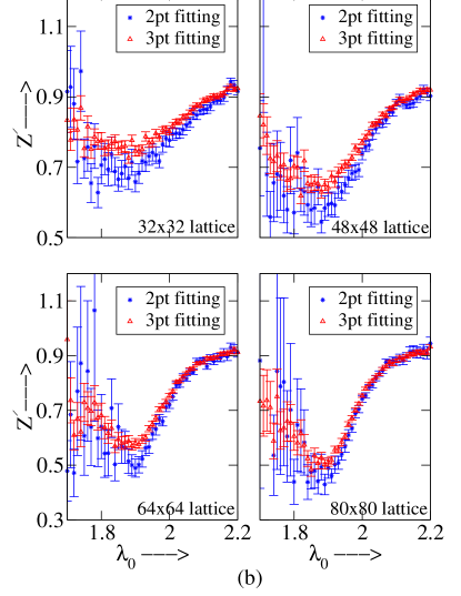
Figure 6: (a) $m_{R^{\prime}}$ in the critical region for different $L$ from momentum space propagator, (b) $Z^{\prime}$ in the critical region for different $L$ from momentum space both for $m_{0}^{2}=-0.5$

Since the calculation of momentum space propagators were extremely time consuming, we had to restrict ourselves to smaller lattices. For thermalization $10^{5}$ configurations were discarded before starting the measurements. The number and size of bins as well as the hop-length were the same as that for coordinate space propagators.

As the inverse propagator was found to be nonlinear in the small momenta region, one could use only the lowest few momentum modes for the determination of $m_{R^{\prime}}$ and $Z^{\prime}$. For this calculation we took the lowest $2$ and $3$ modes excluding the zero momentum mode because the connected propagator value for the zero mode is prone to relatively large statistical error arising from the subtraction, in the critical region, between two quantities measured independently bdwnw . In Figs. 6 (a) and (b), we have presented $m_{R^{\prime}}$ and $Z^{\prime}$ extracted from momentum space propagator with $m_{0}^{2}=-0.5$ for four different lattices. Results obtained using $2$-point and $3$-point fitting are found to be quite close to each other. The $3$-point fitting is more stable and has been used in our study of finite size scaling in the next section.

VI CRITICAL EXPONENTS AND CRITICAL COUPLING FROM FINITE SIZE SCALING ANALYSIS

In this section, we perform a phenomenological Finite Size Scaling (FSS) analysis of our data to extract critical exponents and critical coupling. Let us first briefly summarize the main aspects cardy of this FSS analysis. In a finite size system, there are, in principle, three length scales involved: correlation length $\xi$, size of the system $L$ and the microscopic length $a$ (lattice spacing). FSS assumes that close to a critical point, the microscopic length $a$ drops out. According to FSS brezin , for an observable $P_{L}$ (whose infinite volume limit displays nonanalyticity at the critical point $\lambda_{0}^{c}$), calculated in a finite size of linear dimension $L$,

$$P_{L}(\tau)/P_{\infty}(\tau)=f(L/\xi_{\infty}(\tau))$$ (21)

where $\tau=(\lambda_{0}^{c}-\lambda_{0})/\lambda_{0}^{c}$ and the function $f$ (commonly known as scaling function) is universal in the sense that it does not depend on the type of the lattice, irrelevant operators etc. It does depend on the observable $P$, the geometry, boundary conditions etc. For fixed $L$ as $\tau\rightarrow 0$, strictly there is no phase transition. Consequently $P_{L}(\tau)$ is not singular at $\lambda_{0}=\lambda_{0}^{c}$. Near the critical point we have, $\xi_{\infty}(\tau)=A_{\xi}\tau^{-\nu}$ where $\nu$ is the critical exponent associated with the correlation length. Suppose, near the critical point, $P_{\infty}(\tau)=A_{P}\tau^{-\rho}$. Then from Eq. (21)

$$P_{L}(\tau)=A_{P}\tau^{-\rho}~{}f(A_{\xi}^{-1}L~{}\tau^{\nu})~{}.$$ (22)

Since $P_{L}(\tau)$ should have smooth behavior as $\tau\rightarrow 0$, a simple ansatz for $f$ may be taken as $f(L~{}\tau^{\nu})\sim(L~{}\tau^{\nu})^{\rho/\nu}$ so that $P_{L}(\tau)$ does not blow up as $\tau\rightarrow 0$. Thus $f(x)\sim Cx^{\rho/\nu}$ as $x\rightarrow 0$.

Alternatively, we may write

$$P_{L}(\tau)=A_{P}~{}A_{\xi}^{-\rho/\nu}~{}L^{\rho/\nu}~{}g(A_{\xi}^{-1/\nu}~{}\tau~{}L^{1/\nu}),$$ (23)

where $g$ is another scaling function. Since $P_{L}(\tau)$ should have no singularity as $\tau\rightarrow 0$, $L$ finite, we have, $g(x)\rightarrow{\rm constant}$ as $x\rightarrow 0$.

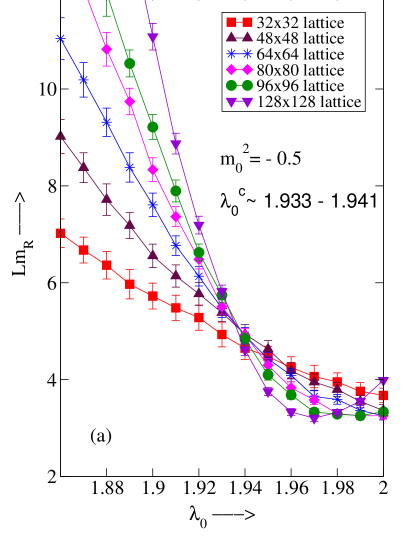
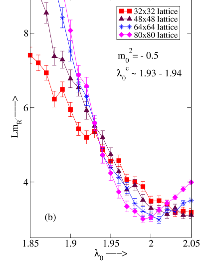
Figure 7: Determination of the critical exponents and critical coupling from finite size scaling analysis of data for $m_{R}$ (or $m_{R^{\prime}}$) in the critical region. $L~{}m_{R}$ and $L~{}m_{R^{\prime}}$ are plotted for different $L$ versus $\lambda_{0}$ with (a) $m_{R}$ extracted from coordinate space propagator data and (b) $m_{R^{\prime}}$ extracted from a 3-point fit near zero momentum of momentum space propagator data

Thus we have

$$L^{\rho/\nu}/P_{L}(\tau)=A_{P}^{-1}~{}A_{\xi}^{\rho/\nu}~{}F(A_{\xi}^{-1/\nu}~{}\tau~{}L^{1/\nu})$$

where the function $F$ is the inverse of the scaling function $g$ and $F(A_{\xi}^{-1/\nu}~{}\tau~{}L^{1/\nu})\rightarrow{\rm a~{}~{}constant}$ as $\tau\rightarrow 0$ for finite $L$. So, we can write

$$L^{\rho/\nu}/P_{L}(\tau)=~{}A_{P}^{-1}~{}A_{\xi}^{\rho/\nu}~{}\left[{\rm C_{P}}~{}+~{}{\rm D_{P}}~{}A_{\xi}^{-1/\nu}~{}\tau~{}L^{1/\nu}~{}+~{}{\cal O}(\tau^{2})\right]$$ (24)

as $\tau\rightarrow 0$ (${\rm C_{P}}$ and ${\rm D_{P}}$ are universal constants in the same sense as the finite size scaling functions). The utility of Eq. (24) is that if we plot $L^{\rho/\nu}/P_{L}\left(\tau\right)$ versus the coupling $\lambda_{0}$ for different values of $L$, all the curves will pass through the same point when $\tau=0$ or equivalently $\lambda_{0}=\lambda_{0}^{c}$ goldenfeld . These ideas provide us with a very good method for evaluating the critical point and checking the critical exponents.

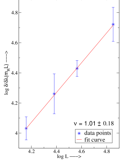
Figure 8: Determination of critical exponent ($\nu$) for mass gap obtained from coordinate space propagator for $m_{0}^{2}=-0.5$.

We have performed finite size scaling analysis for the observables $~{}{\langle\phi\rangle}^{-1},~{}{m_{R}}^{-1}~{}({\rm or}~{}~{}{m_{R^{\prime}}}^{-1})$ and ${Z}^{-1}~{}({\rm or}~{}~{}{Z^{\prime}}^{-1})$. The critical behavior of $\langle\phi\rangle,~{}~{}m_{R}$ and $Z$ may be written as

$$\langle\phi\rangle = A_{\phi}^{-1}~{}\tau^{\beta}$$

$$m_{R} = A_{\xi}^{-1}~{}\tau^{\nu}$$

$$Z = A_{Z}^{-1}~{}\tau^{\eta}~{}.$$ (25)

From the general expectation that in $1+1$ dimensions, $\phi^{4}$ theory and Ising model belong to the same universality class, we have used the Ising values for the corresponding exponents as inputs in our FSS analysis. Thus, $\beta=0.125,~{}\nu=1$ and $\eta=0.25$.

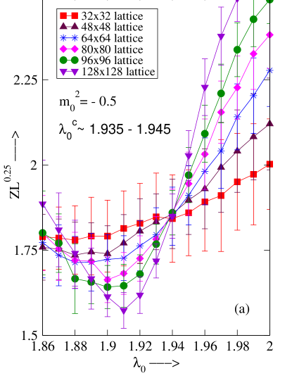
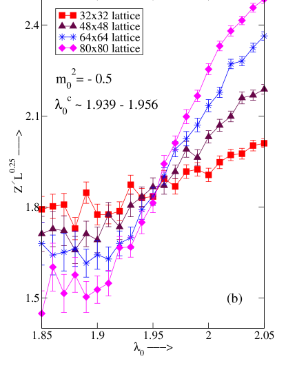
Figure 9: Determination of the critical exponents and critical coupling from finite size scaling analysis of data for $Z$ (or $Z^{\prime}$) in the critical region. $Z~{}L^{0.25}$ and $Z^{\prime}~{}L^{0.25}$ are plotted for different $L$ versus $\lambda_{0}$ with (a) $Z$ extracted from coordinate space propagator and (b) $Z^{\prime}$ extracted from a 3-point fit near zero momentum of the momentum space propagator data.

According to the discussion following Eq. (24), we have plotted $L^{\rho/\nu}/P_{L}(\tau)$ as a function of $\lambda_{0}$ near $\lambda_{0}^{c}$ for different $L$, with $~{}P_{L}(\tau)={m_{R}}^{-1},~{}Z^{-1}$ and $~{}{\langle\phi\rangle}^{-1}$ respectively. Figs. 7(a) and (b) show the plots of $Lm_{R}$ and $Lm_{R^{\prime}}$ for different values of $L$ against $\lambda_{0}$ with $m_{R}$ and $m_{R^{\prime}}$ obtained from coordinate and momentum space propagators respectively. All results are with $m_{0}^{2}=-0.5$. We can clearly identify the critical point with remarkable precision from these plots and this agrees well with the value shown in Fig. 1. Since in this case $\rho=\nu$, we cannot verify the critical exponent for $m_{R}$ (or $m_{R^{\prime}}$) solely from these plots. However, on differentiating goldenfeld , Eq. (24) (with $P_{L}(\tau)=1/m_{R}$) with respect to $\lambda_{0}~{}$ we get

$$\frac{\partial}{\partial\lambda_{0}}\left(L~{}m_{R}\right)=BL^{1/\nu}{\rm as}~{}\tau~{}\rightarrow~{}0,$$

where $B$ is a constant. The exponent $\nu$ can be computed easily by taking the logarithm of the above equation:

$$\log\frac{\partial}{\partial\lambda_{0}}\left(L~{}m_{R}\right)=\log B~{}+~{}\frac{1}{\nu}\log L.$$ (26)

Determination of $\nu$ using Eq. (26) is presented in Fig. 8. In this calculation, we have used the lattice data obtained from coordinate space propagator for four largest lattices $\left(64^{2},~{}80^{2},~{}96^{2},~{}128^{2}\right)$. The value of $\nu$ extracted from our fitting is $1.01\pm 0.18$ which is consistent with the Ising value $(\nu=1)$ to our numerical accuracy.

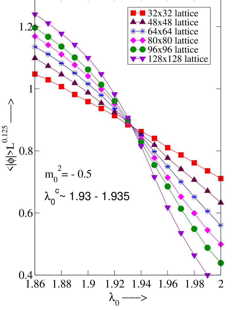
Figure 10: $\langle|\phi|\rangle~{}L^{0.125}$ for different $L$ versus $\lambda_{0}$.

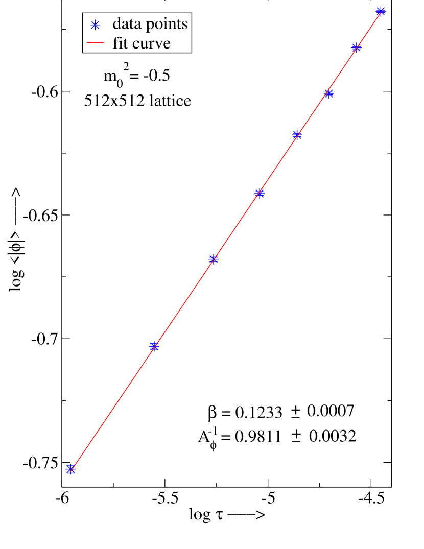
Figure 11: Extraction of critical exponent associated with the order parameter.

Fig. 7 (a) and (b) also give the value of the universal constant $C_{\xi}$ appearing in Eq. (24). Applying Eq. (24) for the case of $m_{R}$, we find at $\tau=0$

$$L~{}m_{R}=A_{\xi}^{-1}~{}A_{\xi}~{}C_{\xi}=C_{\xi}$$ (27)

because $\rho=\nu$. Discarding the $32^{2}$ data which seem not to conform to FSS, from Fig. 7 (a) we find that $C_{\xi}\approx 5.1$. Data in Fig. 7 (b) is noisy; however, it still gives a value around 5.5.

Plots of $Z~{}L^{0.25}$ and $Z^{\prime}~{}L^{0.25}$ against $\lambda_{0}$ for lattices of different lengths $L$ with $Z$ and $Z^{\prime}$ computed from coordinate and momentum space propagators are presented in Figs. 9(a) and (b) respectively. We also present the plots of $\langle|\phi|\rangle~{}L^{0.125}$ against $\lambda_{0}$ for different lattice sizes in Fig. 11. Critical points obtained from all these FSS plots are very close to each other. These plots also provide a very good confirmation of the critical exponents for $Z$ and order parameter $\langle|\phi|\rangle$.

The critical exponent for $\langle|\phi|\rangle$ is also determined by fitting our data for the largest lattice ($512^{2}$) at $m_{0}^{2}=-0.5$ to the corresponding scaling formula for $\langle|\phi|\rangle$. As is shown in Fig. 11, the fit is very satisfactory and the results for the critical exponent and the amplitude are:

$$\beta=0.1233\pm 0.0007~{}~{}~{}~{}~{}{\rm and}~{}~{}~{}~{}~{}~{}A_{\phi}^{-1}=0.9811\pm 0.0032~{}~{}~{}~{}~{}~{}(512^{2}~{}~{}~{}{\rm lattice})$$ (28)

Also, the critical exponent obtained from $\langle|\phi|\rangle$ data with $m_{0}^{2}=-1.0$, although not shown here, agrees well with that extracted for $m_{0}^{2}=-0.5$.

Within our numerical accuracy, critical exponent for $\langle|\phi|\rangle$ calculated in the two different ways, namely, the FSS and the direct fit of the scaling formula on the $512^{2}$ lattice, are very close to each other, indicating that $512^{2}$ lattice is as good as the infinite system.

VII Ratios $\lambda_{R}/m_{R}^{2}$ and $\langle\phi_{R}\rangle$

We choose the following definition luwe of $\lambda_{R}$, appropriate for broken phase, in terms of the renormalized scalar mass $m_{R}$ (or $m_{R^{\prime}}$) and the renormalized vacuum expectation value $\langle\phi_{R}\rangle$,

$$\lambda_{R}=3\frac{m_{R}^{2}}{\langle\phi_{R}\rangle^{2}}=3Z\frac{m_{R}^{2}}{\langle\phi\rangle^{2}}.$$ (29)

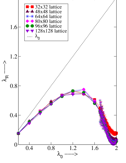
Figure 12: $\lambda_{R}$ for different $L$ from coordinate space propagator for $m_{0}^{2}=-0.5$.

It does not require any knowledge of four point Green function which is computationally demanding. The renormalized coupling $\lambda_{R}$ calculated using $m_{R}$ and $Z$ from coordinate space propagator for six different lattices using the above method is presented in Fig. 12. Error bars are not shown outside the scaling region for the reason explained earlier. As evident from the figure, the renormalized coupling is close to the tree level result in the weak coupling limit. However, $\lambda_{R}$ deviates noticeably from the tree level expectation at stronger couplings; it has a scaling behavior in the critical region and actually vanishes at the critical point modulo finite size effects.

In the previous section, we have already shown that the results of our numerical analysis are consistent with the Ising values of the critical exponents, namely, $\beta=0.125$, $\nu=1$ and $\eta=0.25$. This has the interesting consequence that in 1+1 dimensions, the ratio $\lambda_{R}/m_{R}^{2}$ (or $\lambda_{R}/m_{R^{\prime}}^{2}$) is independent of the bare couplings in the critical region, as follows:

$$\lambda_{R}/{m_{R}}^{2} = 3/{\langle\phi_{R}\rangle}^{2}~{}~{}=~{}~{}3Z/{\langle\phi\rangle}^{2}$$ (30)

$$\sim {(\lambda_{0}^{c}-\lambda_{0})}^{\eta}/{(\lambda_{0}^{c}-\lambda_{0})}^{2\beta}~{}~{}=~{}~{}{(\lambda_{0}^{c}-\lambda_{0})}^{0},$$ (31)

using $\eta=2\beta=0.25$.

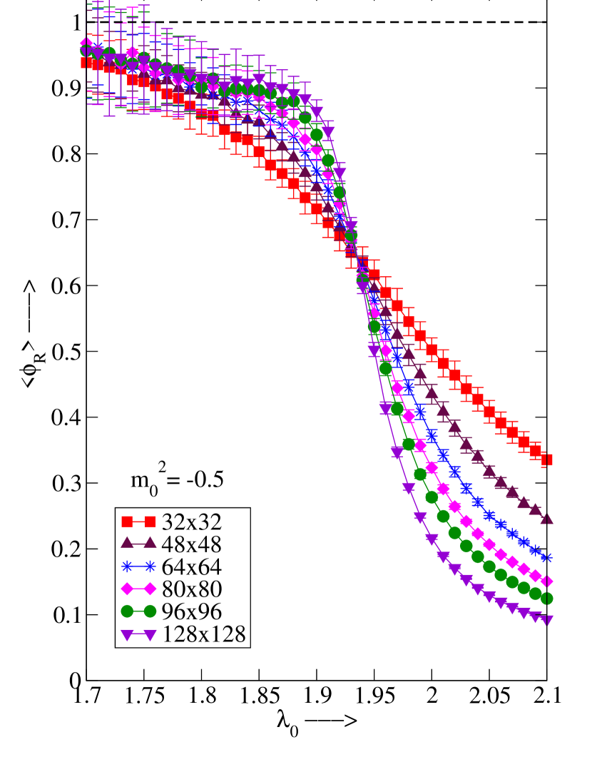
Figure 13: $\langle\phi_{R}\rangle$ versus $\lambda_{0}$ for different $L$ at
$m_{0}^{2}=-0.5$.

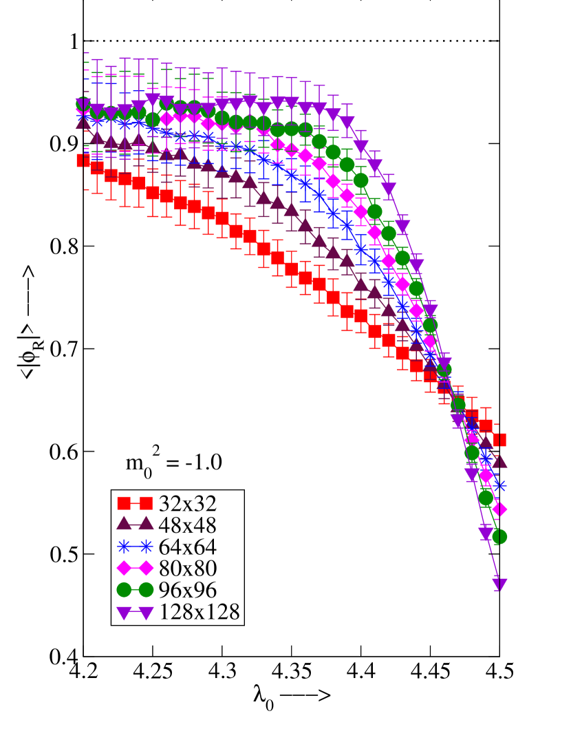
Figure 14: $\langle\phi_{R}\rangle$ versus $\lambda_{0}$ for different $L$ at
$m_{0}^{2}=-1.0$.

In Figs. 14 and 14 for $m_{0}^{2}=-0.5$ and $m_{0}^{2}=-1.0$ respectively, we plot the quantity $\langle\phi_{R}\rangle$ with $Z$ evaluated from coordinate space propagator data, versus $\lambda_{0}$ for six different lattice volumes for a set of bare couplings close to and including the critical region. These figures are consistent with Eq. (31) which shows that in the infinite volume limit $\langle\phi_{R}\rangle$ is independent of the bare couplings. The figures show that for larger lattices the value of $\langle\phi_{R}\rangle$ gets close to unity along a plateau region just away from the critical point in the broken phase and quickly goes to a value close to zero on the symmetric phase side. Judging from the trend in these figures, we expect the curve in the infinite volume limit to take the shape of a step function at the critical point with $\langle\phi_{R}\rangle$ dropping from around unity to zero as it passes the critical point from the broken symmetry phase to the symmetric phase.

One can also try to take the infinite volume limit of $\langle\phi_{R}\rangle$ in the scaling region (as will be shown in the following for the ratio $\lambda_{R}/m_{R}^{2}$ in Figs. 16 and 16). From our extrapolations, although not shown here and already quite apparent from Figs. 14 and 14, this value seems to be very close to unity.

Eq. (30) then immediately tells us that the infinite volume limit of $\lambda_{R}/m_{R}^{2}$ in the scaling region would be close to 3. This is what is indicated in Figs. 16 and 16. The significant error bars in our data result mostly from inaccuracies in the determination of the field renormalization constant $Z$ and do not permit us to take a more accurate infinite volume limit. However, the trend is quite unmistakable.

We notice that for both of the two Figs. 14 and 14, the curves for different volumes meet at the same value of around 0.65 of $\langle\phi_{R}\rangle$ at the critical values of $\lambda_{0}$ ($\sim 1.93$ for $m_{0}^{2}=-0.5$ and $\sim 4.46$ for $m_{0}^{2}=-1.0$). To explain this, we need to look at Eq. (24) from which one can write, at $\tau=0$ and finite volume,

$$\langle\phi_{R}\rangle=\frac{\langle\phi\rangle}{\sqrt{Z}}=\frac{\sqrt{A_{Z}}}{A_{\phi}}\frac{C_{\phi}}{\sqrt{C_{Z}}}.$$ (32)

Factors of the lattice linear dimension $L$ cancel between the numerator and the denominator in the above equation. From the scaling laws Eq. (25) we find that the ratio ${\sqrt{A_{Z}}}/{A_{\phi}}$ is the infinite volume limit of $\langle\phi_{R}\rangle$ which we find to be constant irrespective of the parameters of the theory. In addition, because the coefficients $C_{\phi}$ and $C_{Z}$ are constants (they may, however, depend on things like the boundary conditions etc.), the value of $\langle\phi_{R}\rangle$ at $\tau=0$ is also constant irrespective of the parameters and volume, as shown in Figs. 14 and 14 for two sets of bare couplings.

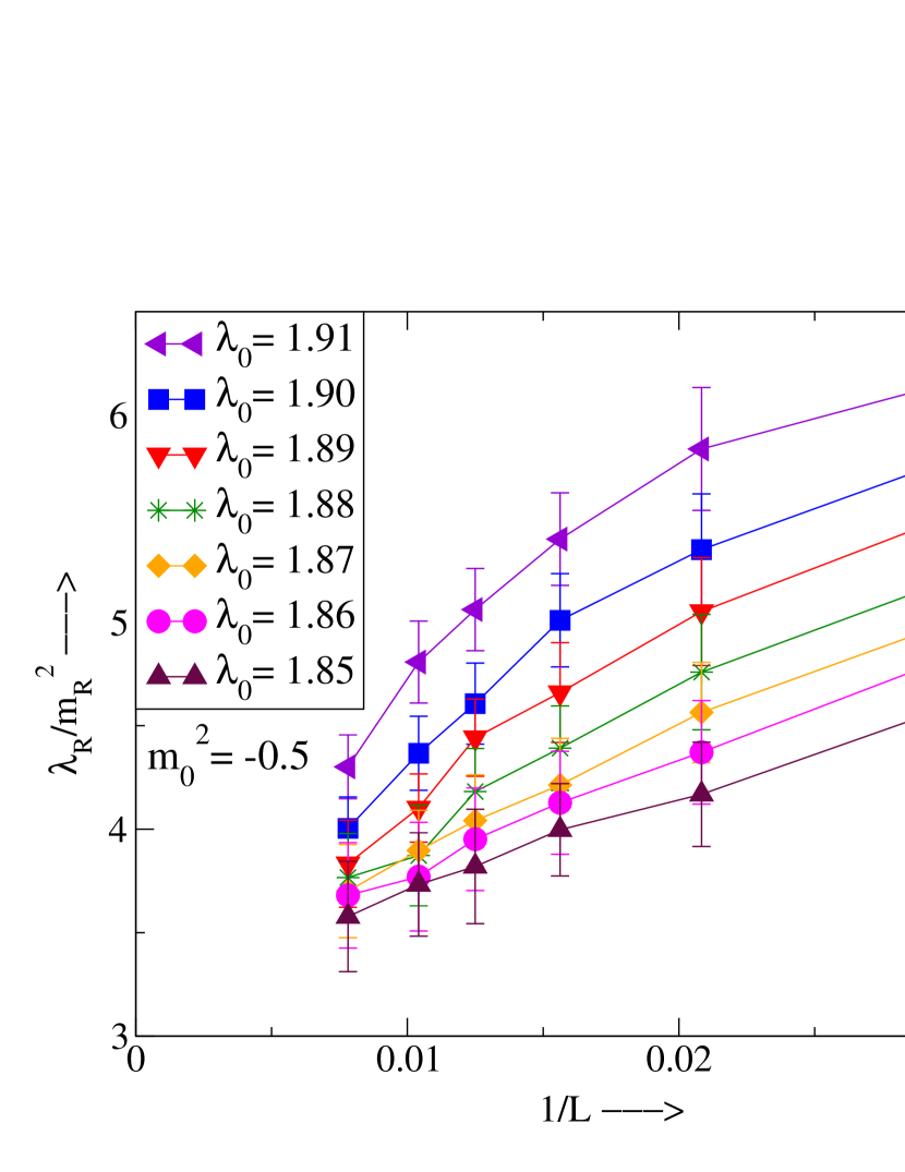
Figure 15: $\lambda_{R}/m_{R}^{2}$ versus $1/L$ for different $\lambda_{0}$ at
$m_{0}^{2}=-0.5$.

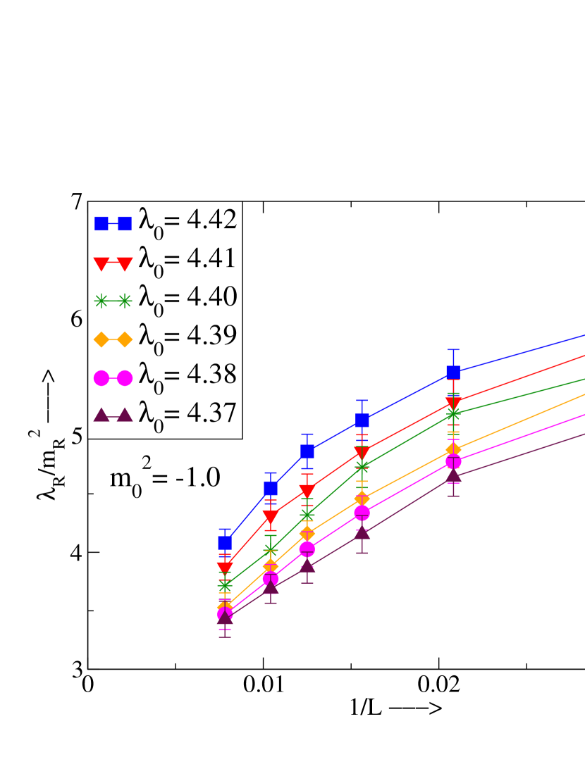
Figure 16: $\lambda_{R}/m_{R}^{2}$ versus $1/L$ for different $\lambda_{0}$ at
$m_{0}^{2}=-1.0$.

VIII Concluding Discussion

Our investigation of the 1+1 dimensional $\phi^{4}$ theory on the lattice has certainly turned out to be more challenging and absorbing than what one would generally expect for a lower dimensional theory.

On the algorithmic front, since the Metropolis algorithm was extremely inefficient near the critical region and for our study we required to obtain a large number of uncorrelated configurations, we had to incorporate the cluster algorithm. Cluster algorithms are generally applicable only to Ising-type systems. In our case, we used a result due to Wolff wolff2 to apply the cluster algorithm to the embedded Ising variables in the $\phi^{4}$ theory. To update the radial modes of the fields the standard Metropolis algorithm had to be blended with the cluster algorithm.

We explored the phase diagram of the lattice theory in two different parameterizations. We have found that symmetry breaking occurs only with a negative mass-squared term in the Hamiltonian.

We needed a large number of configurations to get numerically stable results for the connected propagators in the broken phase. Away from the critical point, the magnitude of the $\phi$ field is large, and the connected propagator which would be a relatively small number had to be extracted from the subtraction of two large numbers. In addition, the momentum space propagators showed signs of curvature for small lattice momenta, a fact which made the determination of the renormalized mass and the field renormalization constant a tough one and we had to be as close to the zero momentum as possible.

Using a definition appropriate for broken symmetry phase, we have calculated the renormalized coupling $\lambda_{R}$ which invloves $m_{R},~{}~{}Z$ and $\langle\phi\rangle$. At weak coupling limit our result is close to the tree level result but deviates significantly in the strong coupling regime.

We have used the finite size scaling analysis to determine the critical point and verify and ultimately determine the critical exponents associated with $m_{R},~{}Z$ and $\langle\phi\rangle$. Verification of critical exponents for $m_{R}$ and $Z$ are performed using the data for both coordinate and momentum space propagators. Apart from verifying the critical exponent for $\langle\phi\rangle$ using FSS analysis, we have also independently determined this quantity by fitting our data for a large enough lattice ($512^{2}$). Our results are consistent with the expectation that in 1+1 dimensions the $\phi^{4}$ theory and the Ising model are in the same universality class.

One of the most important observation in 1+1 dimensions is that the field renormalization constant scales with a particular critical exponent, something that does not happen in 3+1 dimensions. This has the interesting consequence that the renormalized field does not scale and in the infinite volume limit, it drops from a value approximately around unity to zero abruptly as we pass from the broken symmetry phase to the symmetric phase. Moreover, the ratio of the renormalized quartic coupling to the square of the renormalized mass also does not scale and appears to be independent of the bare parameters in the scaling region. Numerically this ratio seems to approach a value around 3 in the infinite volume limit. However, our infinite volume extrapolations are approximate due to large finite size effects and systematic error in the calculation of the field renormalization constant $Z$.

For reliable extrapolation of the above amplitude ratios to infinite volume there exist methods infvol which we have not tried in the present work. We need to have smaller error bars especially on the $m_{R}$ and $Z$ data and this can be taken up in a future work.

- (1) See for example, Shau-Jin Chang, Phys. Rev. D 12, 1071 (1975); P. M. Stevenson, Phys. Rev. D 32, 1389 (1985); L. Polley, U. Ritschel, Phys. Lett. B 221, 44 (1989); P.Cea, L.Tedesco, Phys. Lett. B 335, 423 (1994); J.M. Hauser, W. Cassing, A. Peter, M.H. Thoma, Z. Phys. A 353, 301 (1995); P. J. Marrero, E. A. Roura and D. Lee, Phys. Lett. B 471, 45 (1999); H. Hansen and G. Chanfray, Eur. Phys. J. A 20, 459 (2004); Various light front Hamiltonian studies reviewed in S. J. Brodsky, H.-C. Pauli, S. S. Pinsky, Phys. Rept. 301, 299 (1998).
- (2) W. Loinaz and R. S. Willey, Phys. Rev. D 58, 076003 (1998) [arXiv:hep-lat/9712008].
- (3) Asit K. De, A. Harindranath, Jyotirmoy Maiti and Tilak Sinha, Phys. Rev. D 72, 094504 (2005), arXiv:hep-lat/0506003.
- (4) A.B. Zamolodchikov, Sov. J. Nucl. Phys. 44, 529 (1986).
- (5) Janos Balog, Anthony Duncan, Ray Willey, Ferenc Niedermayer and Peter Weisz, MPP-2004-152, Dec 2004, 15pp; [arXiv:hep-lat/0412015].
- (6) U. Wolff, Int. J. Mod. Phys. C 4 451 (1993), [arXiv:hep-lat/9209005].
- (7) R. C. Brower and P. Tamayo, Phys. Rev. Lett. 62, 1087 (1989).
- (8) U. Wolff, Phys. Rev. Lett. 62, 361 (1989).
- (9) M. Hasenbusch and S. Meyer, Phys. Rev. Lett. 66, 530 (1991); M. Hasenbusch and K. Pinn, Physica A 192, 342 (1993) and private communications from M. Hasenbusch.
- (10) J. C. Ciria and A. Tarancon, Phys. Rev. D 49, 1020 (1994) [arXiv:hep-lat/9309019].
- (11) A. Ardekani and A. G. Williams, Austral. J. Phys. 52, 929 (1999) [arXiv:hep-lat/9811002].
- (12) J. L. Cardy in Finite-Size Scaling, edited by J. L. Cardy, (Elsevier-Science Publishers, B.V., Amsterdam, 1988).
- (13) E. Brézin, J. Phys. (France) 43, 15 (1982); reprinted in Ref. cardy .
- (14) N. Goldenfeld, Lectures on Phase Transitions and the Renormalization Group, (Addison-Wesley Publishing Company, Reading, Massachusetts, 1992).
- (15) M. Lüscher and P. Weisz, Nucl. Phys. 295, 65 (1988).
- (16) S. Caracciolo, R.G. Edwards, S.J. Ferreira, A. Pelissetto and A.D. Sokal, Phys. Rev. Lett. 74 2969 (1995); M. Lüscher, P. Weisz and U. Wolff, Nucl. Phys. B359 221 (1991).