Color Dynamics in External Fields

Abstract:

We investigate the vacuum dynamics of U(1), SU(2), and SU(3) lattice gauge theories in presence of external (chromo)magnetic fields, both in (3+1) and (2+1) dimensions. We find that the critical coupling for the phase transition in compact U(1) gauge theory is independent of the strength of an external magnetic field. On the other hand we find that, both in (3+1) and (2+1) dimensions, the deconfinement temperature for SU(2) and SU(3) gauge systems in a constant abelian chromomagnetic field decreases when the strength of the applied field increases. We conclude that the dependence of the deconfinement temperature on the strength of an external constant chromomagnetic field is a peculiar feature of non abelian gauge theories and could be useful to get insight into color confinement.

1 Introduction

Color confinement is still a puzzling problem not withstanding the large mess of numerical investigations aimed to understand the nature of the QCD vacuum. Indeed, the mechanism that leads to color confinement remains an open question despite intense lattice studies for nearly three decades.

According to a model conjectured long time ago by G. ’t Hooft [1] and S. Mandelstam [2] the confining vacuum behaves as a coherent state of color magnetic monopoles, or, equivalently, the vacuum resembles a magnetic (dual) superconductor. Up to now there is numerical evidence [3, 4, 5, 6, 7, 8, 9, 10, 11, 12] in favor of chromoelectric flux tubes in pure lattice gauge vacuum. As well there have been extensive numerical studies [13, 14, 15, 16, 17, 18, 19, 20, 21, 22, 23, 24] of monopole condensation.

An alternative model for color confinement is based on the special role of center vortices and $Z_{N}$ symmetry (see [25] and references therein), even if the connection of center symmetry to confinement has been recently questioned in [26, 27].

One may conclude that there is no totally convincing explanation of the confinement phenomenon (for recent reviews on confinement see [28, 25, 29]) and that a full understanding of the QCD vacuum dynamics is still lacking. Indeed, as recently observed [30] in connection with dual superconductivity picture, even if magnetic monopoles do condense in the confinement mode, the actual mechanism of confinement could depend on additional dynamical forces. Therefore we feel that it is important to explore any new paths that possibly may suggest new hints for understanding the QCD vacuum.

In a previous paper [31] we reported numerical results showing that in four dimensional U(1) lattice gauge theory the confining vacuum behaves as a coherent condensate of Dirac magnetic monopoles, according to analytical results in the literature [32]. In the same paper we gave account of numerical results indicating condensation of abelian magnetic monopoles and abelian vortices in the confined phase of finite temperature SU(2) and SU(3) lattice gauge theories in (3+1) dimensions. Therefore one might conclude that in SU(2) and SU(3) gauge theories the confining vacuum behaves as a coherent abelian magnetic condensate. We also found [33] that a weak constant abelian chromomagnetic field at zero temperature is completely screened in the continuum limit, while at finite temperature [34, 35] our numerical results indicate that the applied field is restored by increasing the temperature. These results strongly suggested that the confinement dynamics could be intimately related to abelian chromomagnetic gauge configurations. Similar arguments have been reported in ref. [36]. Moreover, in Refs. [34, 35] the SU(3) vacuum was probed by means of an external constant abelian chromomagnetic field with increasing field strength. Remarkably, we found that by increasing the strength of the applied external field the deconfinement temperature decreases towards zero. This means that strong enough abelian chromomagnetic fields destroy the confinement of color. In analogy to what happens in familiar superconductors when the strength of an external magnetic field is increased (see for instance ref. [37]), this effect can be named ”reversible color Meissner effect” . Altough the existence of a critical chromomagnetic field is not easily understandable within the coherent magnetic monopole condensate picture of the confining vacuum, it could be directly explained if the vacuum behaves as an ordinary relativistic color superconductor, or differently stated, if the confining vacuum resembles as a coherent condensate of tachionic color charged scalar fields. Thus we have to reconcile two apparently different aspects. From one hand, the confining vacuum does display condensation of both abelian magnetic monopoles and vortices, on the other hand the relation between the deconfinement temperature and the applied abelian chromomagnetic field suggested that the vacuum behaves as a condensate of an effective color charged scalar field whose mass is proportional to the inverse of the magnetic length [34, 35]. The reversible color Meissner effect could be in agreement with R. P. Feynman who, in a seminal paper [38], argued that in three dimensional SU(2) gauge theory long range correlation between gluonic degrees of freedom destroys confinement. We would like to point out, to avoid misunderstanding, that our reversible color Meissner effect is not related to color superconductivity in cold dense quark matter (for a recent review see ref. [39] and references therein).

The aim of the present paper is to investigate if our reversible color Meissner effect is a generic feature of non abelian gauge theories. To this end, we shall compare SU(3) and SU(2) gauge theories in an external abelian chromomagnetic field both in (3+1) and (2+1) dimensions. We shall, also, consider three and four dimensional U(1) gauge theories in a magnetic background field.

The plan of the paper is as follows. In sect. 2 we briefly recall for reader convenience our proposal of lattice effective action and define the abelian chromomagnetic field on the lattice. In sect. 3 we present our results on vacuum dynamics in an external chromomagnetic background field in (3+1)-dimensions for SU(3) and SU(2) at finite temperature, and for U(1) at zero temperature. Sect. 4 is devoted to corresponding results in (2+1)-dimensions. Finally in sect. 5 we summarize and conclude. In Appendix A we present results for SU(3) in an external chromomagnetic background field directed along the direction $\hat{8}$ in color space.

2 The gauge invariant lattice effective action

In our previous studies, in order to investigate vacuum structure of lattice gauge theories both at zero and finite temperature, we introduced a lattice effective action for gauge systems in external static background fields. In this section, for reader convenience, we shall briefly summarize our proposal of lattice effective action which is gauge invariant against static gauge transformations of the background field.

2.1 The lattice effective action: $T=0$

In Refs. [40, 33] we introduced a lattice gauge invariant effective action $\Gamma[\vec{A}^{\text{ext}}]$ for an external background field $\vec{A}^{\text{ext}}$:

$$\Gamma[\vec{A}^{\text{ext}}]=-\frac{1}{L_{t}}\ln\left\{\frac{{\mathcal{Z}}[\vec{A}^{\text{ext}}]}{{\mathcal{Z}}[0]}\right\}$$ (1)

where $L_{t}$ is the lattice size in time direction and $\vec{A}^{\text{ext}}(\vec{x})$ is the continuum gauge potential of the external static background field. ${\mathcal{Z}}[\vec{A}^{\text{ext}}]$ is the lattice partition functional

$${\mathcal{Z}}[\vec{A}^{\text{ext}}]=\int_{U_{k}(\vec{x},x_{t}=0)=U_{k}^{\text{ext}}(\vec{x})}{\mathcal{D}}U\;e^{-S_{W}}\,,$$ (2)

with $S_{W}$ the standard pure gauge Wilson action.

The functional integration is performed over the lattice links, but constraining the spatial links belonging to a given time slice (say $x_{t}=0$) to be

$$U_{k}(\vec{x},x_{t}=0)=U^{\text{ext}}_{k}(\vec{x})\,,\,\,\,\,\,(k=1,2,3)\,\,,$$ (3)

$U^{\text{ext}}_{k}(\vec{x})$ being the lattice version of the external continuum gauge potential $\vec{A}^{\text{ext}}(x)=\vec{A}^{\text{ext}}_{a}(x)\lambda_{a}/2$. Note that the temporal links are not constrained.

In the case of a static background field which does not vanish at infinity we must also impose that, for each time slice $x_{t}\neq 0$, spatial links exiting from sites belonging to the spatial boundaries are fixed according to eq. (3). In the continuum this last condition amounts to the requirement that fluctuations over the background field vanish at infinity.

The partition function defined in eq. (2) is also known as lattice Schrödinger functional [41, 42] and in the continuum corresponds to the Feynman kernel [43]. Note that, at variance with the usual formulation of the lattice Schrödinger functional [41, 42] where a lattice cylindrical geometry is adopted, our lattice has an hypertoroidal geometry so that $S_{W}$ in eq. (2) is allowed to be the standard Wilson action.

The lattice effective action $\Gamma[\vec{A}^{\text{ext}}]$ corresponds to the vacuum energy, $E_{0}[\vec{A}^{\text{ext}}]$, in presence of the background field with respect to the vacuum energy, $E_{0}[0]$, with $\vec{A}^{\text{ext}}=0$

$$\Gamma[\vec{A}^{\text{ext}}]\quad\longrightarrow\quad E_{0}[\vec{A}^{\text{ext}}]-E_{0}[0]\,.$$ (4)

The relation above is true by letting the temporal lattice size $L_{t}\to\infty$; on finite lattices this amounts to have $L_{t}$ sufficiently large to single out the ground state contribution to the energy.

Since the lattice effective action eq. (1) is given in terms of the lattice Schrödinger functional, which is invariant for time-independent gauge transformation of the background field [41, 42], it is gauge invariant too.

2.2 The thermal partition functional

If we now consider the gauge theory at finite temperature $T=1/(aL_{t})$ in presence of an external background field, the relevant quantity turns out to be the free energy functional defined as

$${\mathcal{F}}[\vec{A}^{\text{ext}}]=-\frac{1}{L_{t}}\ln\left\{\frac{{\mathcal{Z_{T}}}[\vec{A}^{\text{ext}}]}{{\mathcal{Z_{T}}}[0]}\right\}\;.$$ (5)

${\mathcal{Z_{T}}}[\vec{A}^{\text{ext}}]$ is the thermal partition functional [44] in presence of the background field $\vec{A}^{\text{ext}}$, and is defined as

$$\mathcal{Z}_{T}\left[\vec{A}^{\text{ext}}\right]=\int_{U_{k}(\vec{x},L_{t})=U_{k}(\vec{x},0)=U^{\text{ext}}_{k}(\vec{x})}\mathcal{D}U\,e^{-S_{W}}\,.$$ (6)

In eq. (6), as in eq. (2), the spatial links belonging to the time slice $x_{t}=0$ are constrained to the value of the external background field, the temporal links are not constrained. On a lattice with finite spatial extension we also usually impose that the links at the spatial boundaries are fixed according to boundary conditions eq. (3), apart from the case in which the external background field vanishes at spatial infinity (as happens for the monopole field), where the choice of periodic boundary conditions in the spatial direction is equivalent to eq. (3) in the thermodynamical limit. If the physical temperature is sent to zero, the thermal functional eq. (6) reduces to the zero-temperature Schrödinger functional eq. (2). The free energy functional eq. (5) corresponds to the free energy, $F[\vec{A}^{\text{ext}}]$, in presence of the external background field evaluated with respect to the free energy, $F[0]$, with $\vec{A}^{\text{ext}}=0$. When the physical temperature is sent to zero the free energy functional reduces to the vacuum energy functional eq. (1).

2.3 Abelian (chromo)magnetic background field

We are interested in vacuum dynamics of U(1), SU(2), and SU(3) lattice gauge theories under the influence of an abelian chromomagnetic background field.

In our previous studies we found that in SU(2) and SU(3) at zero temperature a (not too strong) constant abelian chromomagnetic field at zero temperature is completely screened in the continuum limit [33]. We also found that in SU(3) the deconfinement temperature depends on the strength of an applied external constant abelian chromomagnetic field [35]. This is at variance of abelian magnetic monopoles where the abelian monopole background fields do not modify the deconfinement temperature [45]. We would like to corroborate our findings with further investigations, in particular we would like to ascertain if the dependence of the deconfinement temperature on the strength of an applied external constant abelian chromomagnetic field is a peculiar feature of non abelian gauge theories.

Let us now define a static constant abelian chromomagnetic field on the lattice. We first consider the SU(3) case. In the continuum the gauge potential giving rise to a static constant abelian chromomagnetic field directed along spatial direction $\hat{3}$ and direction $\tilde{a}$ in the color space is given by

$$\vec{A}^{\text{ext}}_{a}(\vec{x})=\vec{A}^{\text{ext}}(\vec{x})\delta_{a,\tilde{a}}\,,\quad A^{\text{ext}}_{k}(\vec{x})=\delta_{k,2}x_{1}H\,.$$ (7)

In SU(3) lattice gauge theory the constrained lattice links (see eq. (3)) corresponding to the continuum gauge potential eq. (7) are (choosing $\tilde{a}=3$, i.e. abelian chromomagnetic field along direction $\hat{3}$ in color space)

$$\begin{split}&U^{\text{ext}}_{1}(\vec{x})=U^{\text{ext}}_{3}(\vec{x})={\mathbf{1}}\,,\\ &U^{\text{ext}}_{2}(\vec{x})=\begin{bmatrix}\exp(i\frac{gHx_{1}}{2})&0&0\\ 0&\exp(-i\frac{gHx_{1}}{2})&0\\ 0&0&1\end{bmatrix}\,.\end{split}$$ (8)

We will refer to this case as $T_{3}$ abelian chromomagnetic field. If we choose instead abelian chromomagnetic field along direction $\hat{8}$ in color space the constrained lattice links are given by

$$\begin{split}&U^{\text{ext}}_{1}(\vec{x})=U^{\text{ext}}_{3}(\vec{x})={\mathbf{1}}\\ &U^{\text{ext}}_{2}(\vec{x})=\begin{bmatrix}\exp(i\frac{gHx_{1}}{2\sqrt{3}})&0&0\\ 0&\exp(i\frac{gHx_{1}}{2\sqrt{3}})&0\\ 0&0&\exp(-i\frac{gHx_{1}}{\sqrt{3}})\end{bmatrix}\,.\end{split}$$ (9)

We will refer to this case as $T_{8}$ abelian chromomagnetic field. Since our lattice has the topology of a torus, the magnetic field turns out to be quantized

$$a^{2}\frac{gH}{2}=\frac{2\pi}{L_{1}}n_{\text{ext}}\,,\qquad n_{\text{ext}}\,\,\,{\text{integer}}\,.$$ (10)

In the case of SU(2) lattice gauge theories the constrained spatial links are

$$\begin{split}&U^{\text{ext}}_{1}(\vec{x})=U^{\text{ext}}_{3}(\vec{x})={\mathbf{1}}\,,\\ &U^{\text{ext}}_{2}(\vec{x})=\cos(\frac{gHx_{1}}{2})+i\sigma^{3}\sin(\frac{gHx_{1}}{2})\,,\end{split}$$ (11)

$\sigma^{3}$ being the Pauli matrix.
Finally in the U(1) case the constrained spatial links corresponding to a constant magnetic background field (along spatial direction $\hat{3}$) are

$$\begin{split}&U^{\text{ext}}_{1}(\vec{x})=U^{\text{ext}}_{3}(\vec{x})={\mathbf{1}}\,,\\ &U^{\text{ext}}_{2}(\vec{x})=\cos(gHx_{1})+i\sin(gHx_{1})\,.\end{split}$$ (12)

Since the free energy functional $F[\vec{A}^{\text{ext}}]$ is invariant for time independent gauge transformations of the background field $\vec{A}^{\text{ext}}$, it follows that for a constant background field, $F[\vec{A}^{\text{ext}}]$ is proportional to the spatial volume $V=L_{s}^{3}$, and the relevant quantity is the density $f[\vec{A}^{\text{ext}}]$ of free energy

$$f[\vec{A}^{\text{ext}}]=\frac{1}{V}F[\vec{A}^{\text{ext}}]\,.$$ (13)

We evaluate by numerical simulations the derivative with respect to the coupling $\beta$ of the free energy density $f[\vec{A}^{\text{ext}}]$ at fixed external field strength $gH$

$$f^{\prime}[\vec{A}^{\text{ext}}]=\left\langle\frac{1}{\Omega}\sum_{x,\mu<\nu}\frac{1}{3}\,\text{Re}\,{\text{Tr}}\,U_{\mu\nu}(x)\right\rangle_{0}\\ -\left\langle\frac{1}{\Omega}\sum_{x,\mu<\nu}\frac{1}{3}\,\text{Re}\,{\text{Tr}}\,U_{\mu\nu}(x)\right\rangle_{\vec{A}^{\text{ext}}}\,,$$ (14)

where the subscripts on the averages indicate the value of the external field and $\Omega=L_{s}^{3}\times L_{t}$ is the lattice volume. The generic plaquette $U_{\mu\nu}(x)=U_{\mu}(x)U_{\nu}(x+\hat{\mu})U^{\dagger}_{\mu}(x+\hat{\nu})U^{\dagger}_{\nu}(x)$ contributes to the sum in eq. (14) if the link $U_{\mu}(x)$ is a ”dynamical” one, i.e. it is not constrained in the functional integration eq. (6). Observing that $f[\vec{A}^{\text{ext}}]=0$ at $\beta=0$, we may eventually obtain $f[\vec{A}^{\text{ext}}]$ from $f^{\prime}[\vec{A}^{\text{ext}}]$ by numerical integration:

$$f[\vec{A}^{\text{ext}}]=\int_{0}^{\beta}f^{\prime}[\vec{A}^{\text{ext}}]\,d\beta^{\prime}\;.$$ (15)

3 (3+1) dimensions

In this section we report results obtained in studying the finite temperature phase transition of lattice gauge theories SU(3) and SU(2) in (3+1)-dimensions, in presence of a constant abelian chromomagnetic background field. We shall also report results for confinement-Coulomb phase transition in U(1) lattice gauge theory at zero temperature in a constant magnetic background field. A preliminary account of our results has ben presented in ref. [46].

3.1 SU(3)

We simulate SU(3) pure gauge theory in a constant abelian background field defined in Eqs. (7) and (8). As is well known, the pure SU(3) gauge system undergoes a deconfinement phase transition at a given critical temperature. Our aim is to study the possible dependence of the critical temperature from the strength of the applied field. The critical coupling $\beta_{c}$ can be evaluated by measuring $f^{\prime}[\vec{A}^{\text{ext}}]$, the derivative of the free energy density with respect to $\beta$, as a function of $\beta$. Indeed we found that $f^{\prime}[\vec{A}^{\text{ext}}]$ (see eq. (14)) displays a peak in the critical region (see fig. 1) where it can be parameterized as

$$\frac{f^{\prime}(\beta,L_{t})}{\varepsilon^{\prime}_{\text{ext}}}=\frac{a_{1}(L_{t})}{a_{2}(L_{t})[\beta-\beta^{*}(L_{t})]^{2}+1}\,.$$ (16)

In eq. (16) we normalize $f^{\prime}$ to $\varepsilon^{\prime}_{\text{ext}}$, the derivative of the classical energy due to the external applied field

$$\varepsilon^{\prime}_{\text{ext}}=\frac{2}{3}\,[1-\cos(\frac{gH}{2})]=\frac{2}{3}\,[1-\cos(\frac{2\pi}{L_{1}}n_{\text{ext}})]\,.$$ (17)

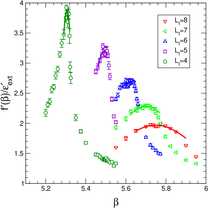
Figure 1: SU(3) in (3+1) dimensions. The derivative of the free energy density with respect to the gauge coupling $\beta$, eq. (14), versus $\beta$ at fixed external field strength ($n_{\text{ext}}=1$) for spatial lattice size $L_{s}=64$ and temporal lattice sizes $L_{t}=4,5,6,7,8$. Solid lines are the fits eq. (16).

Remarkably, we have checked that the evaluation of the critical coupling $\beta^{*}(L_{t})$ by means of $f^{\prime}[\vec{A}^{\text{ext}}]$ is consistent with the usual determination obtained through the temporal Polyakov loop susceptibility:

$$\begin{split}&\chi(|P|)=<|P|^{2}>-<|P|>^{2}\\ &P=\frac{1}{V_{s}}\sum_{\vec{x}}\frac{1}{3}\,{\text{Tr}}\prod_{x_{4}=1}^{L_{t}}U_{4}(x_{4},\vec{x})\,.\end{split}$$ (18)

The Polyakov loop susceptibility near the peak has been obtained by means of the density spectral method [47, 48]. The statistical errors for the points belonging to the extrapolated curve near the peak, as well as the position of the peak and its statistical error, were evaluated by means of a bootstrap analysis [49]. For instance, on a $64^{3}\times 6$ lattice and $n_{\text{ext}}=1$ we get $\beta_{c}=5.6272(69)$ from eq. (16) and $\beta_{c}=5.6266(12)$ when evaluating the peak of the Polyakov loop susceptibility by means of the density spectral method (see fig. 2).

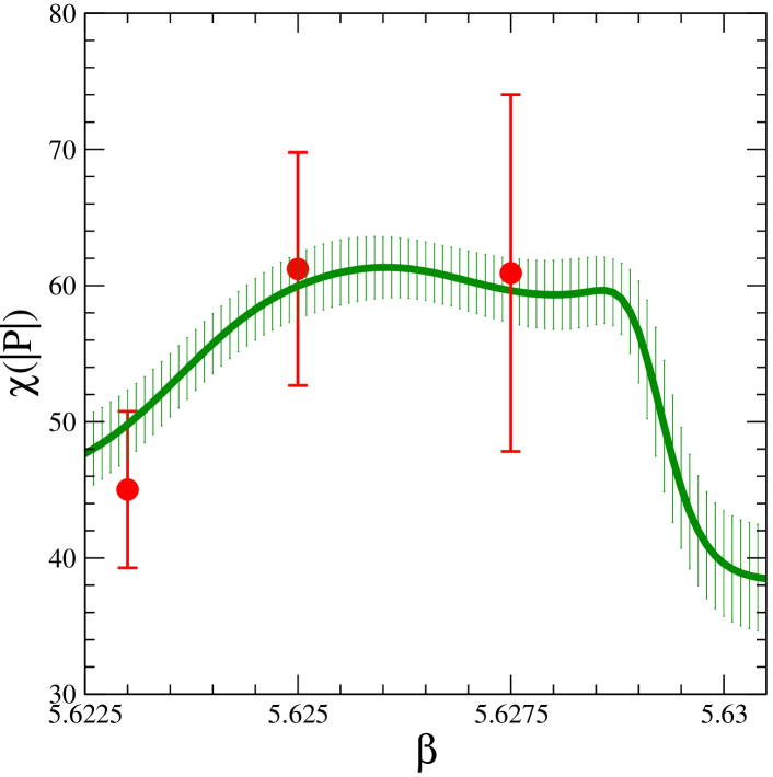
Figure 2: SU(3) in (3+1) dimensions. The susceptibility of the absolute value of the Polyakov loop evaluated for three values of $\beta$ on a $64^{3}\times 6$ lattice and external field strength $n_{\text{ext}}=1$. The solid line has been obtained by reweighting. The error bars have been estimated using the bootstrap method.

Once $\beta^{*}(L_{t})$ has been determined, the deconfinement temperature can be preliminarily estimated in units of $\Lambda_{\text{latt}}$. Indeed

$$\frac{T_{c}}{\Lambda_{\text{latt}}}=\frac{1}{L_{t}}\frac{1}{f_{SU(3)}(\beta^{*}(L_{t}))}\,,$$ (19)

where

$$f_{SU(N)}(\beta)=\left(\frac{\beta}{2Nb_{0}}\right)^{b_{1}/2b_{0}^{2}}\,\exp\left(-\beta\frac{1}{4Nb_{0}}\right)\,,$$ (20)

$N$ being the color number, $b_{0}=(11N)/(48\pi^{2})$, and $b_{1}=(34N^{2})/(3(16\pi^{2})^{2})$. In order to obtain the continuum limit of the critical temperature we have to extrapolate $T_{c}/\Lambda_{\text{latt}}$, given by eq. (19), to the continuum. This can be done, following ref. [50], by means of a linear extrapolation of $T_{c}/\Lambda_{\text{latt}}$ as a function of $aT_{c}$ for $aT_{c}\to 0$. We varied the strength of the applied external abelian chromomagnetic background field to study quantitatively the dependence of $T_{c}$ on $gH$.

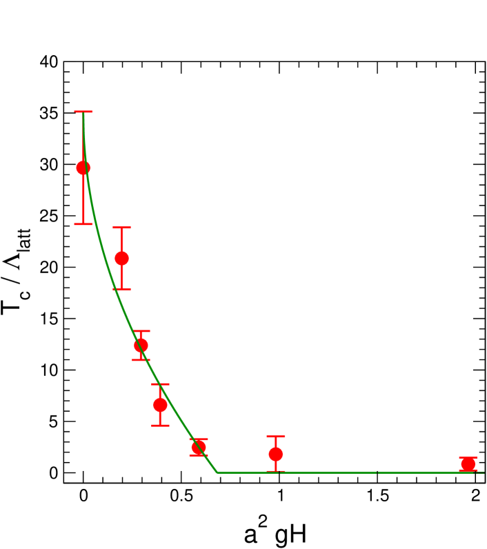
Figure 3: SU(3) in (3+1) dimensions. The continuum critical temperature $T_{c}$ in units of $\Lambda_{\text{latt}}$ versus the external field strength eq. (10) (in lattice units). Solid line is the fit eq. (22) to our data.

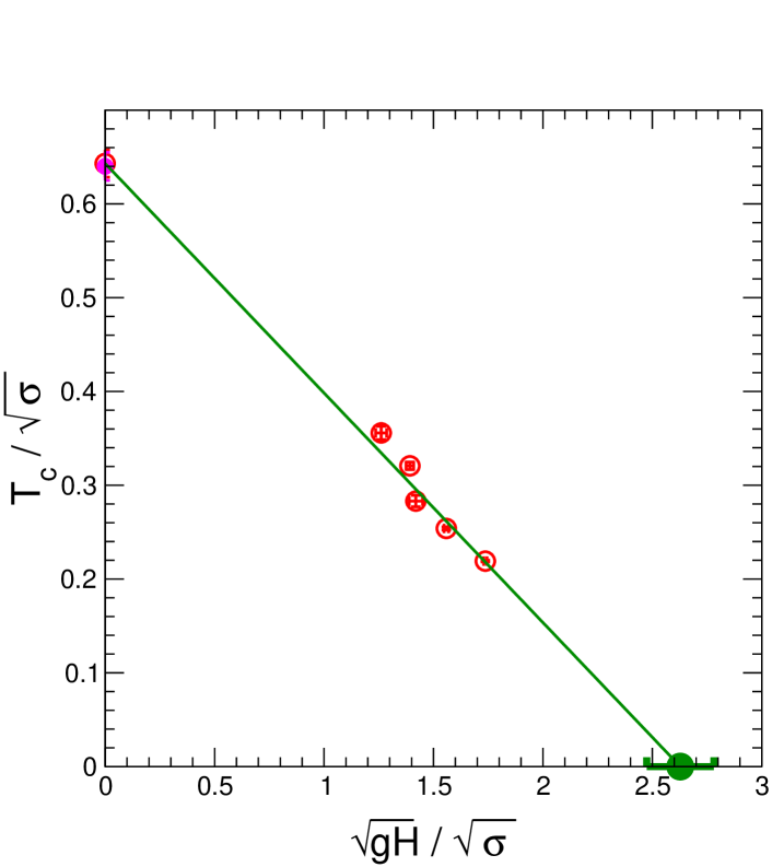
Figure 4: SU(3) in (3+1) dimensions. The critical temperature $T_{c}$ estimated on a $64^{3}\times 8$ lattice in units of the string tension, eq. (25), versus the square root of the field strength $\sqrt{gH}$ in units of the string tension, eq. (26). Solid line is the linear fit eq. (27). In correspondence of zero vertical axis: open circle is $T_{c}/\sqrt{\sigma}$ at zero external field, Eq. (28); full circle is the determination of $T_{c}/\sqrt{\sigma}$ obtained in the literature [51] The green full point is the critical field in units of the string tension, eq. (29).

From fig. 3, where we display $T_{c}/\Lambda_{\text{latt}}$ versus $gH$ in lattice units, we may conclude that the critical temperature decreases by increasing the strength of the external abelian chromomagnetic field and eventually goes to zero for a strong enough external field.

To get more insight into this result we can try to parameterize the behavior of the critical temperature versus the applied field strength. As a matter of fact, if the magnetic length, defined as $a_{H}\sim 1/\sqrt{gH}$, is the only relevant scale of the problem for dimensional reasons one expects that

$$T_{c}^{2}\,\,\sim\,\,gH\,.$$ (21)

Indeed, as fig. 3 displays, we get a good fit to our data using the following parameterization

$$\frac{T_{c}(gH)}{\Lambda_{\text{latt}}}=\frac{T_{c}(0)}{\Lambda_{\text{latt}}}+\alpha\sqrt{a^{2}gH}\,.$$ (22)

We get

$$\begin{split}&T_{c}(0)/\Lambda_{\text{latt}}=35.5\pm 5.2\\ &\alpha=-42.4\pm 7.4\,.\end{split}$$ (23)

It is worthwhile to note that our estimation for $T_{c}(0)/\Lambda_{\text{latt}}$ is compatible with $T_{c}(0)/\Lambda_{\text{latt}}=29.67\pm 5.47$ obtained in ref. [50] with completely different methods.

The preliminary analysis of our lattice data drives us to conclude that, remarkably, a critical field, $gH_{c}\simeq 0.68$ (in lattice units), exists such that $T_{c}=0$ for $gH>gH_{c}$. This kind of behavior could be interpreted as the colored counterpart of the Meissner effect in ordinary superconductors, when strong enough magnetic fields destroy the superconductive BCS vacuum [37]. Then we shall refer to this remarkable result as the reversible color Meissner effect. Once again we would like to stress that this effect is not related to the color superconductivity in cold dense quark matter. Indeed, we believe that our reversible color Meissner effect is deeply rooted in the non-perturbative color confining nature of the vacuum and could be a window open towards unraveling the true nature of the confining vacuum.

So far we reported our results for the critical temperature $T_{c}$ in units of $\Lambda_{\text{latt}}$ and for the critical strength of the abelian chromomagnetic background field in lattice units. However it is well known that asymptotic scaling could be affected by scaling violation effects due to finite size of the lattice. On the other hand, such as effects are strongly reduced in the scaling of physical quantities. So that it is useful to analyze our data in physical units. In a pure gauge theory this can be done in terms of the string tension $\sigma$ computed at zero temperature in correspondence of the value of the gauge coupling $\beta=\beta_{c}$. We do not need to directly compute the string tension, for we may use the following parameterization of the SU(3) string tension given by Edwards et al. (see eq. (4.4) in ref. [52])

$$\begin{split}&(a\sqrt{\sigma})(g)=\,f_{SU(3)}(g^{2})~{}(\,1+0.2731\,\hat{a}^{2}(g)-0.01545\,\hat{a}^{4}(g)+0.01975\,\hat{a}^{6}(g)\,)/0.01364\,,\\ &\hat{a}(g)=\frac{f_{SU(3)}(g^{2})}{f_{SU(3)}(g^{2}(\beta=6))}\,;\qquad\beta=\frac{6}{g^{2}}\,,\end{split}$$ (24)

for $5.6\leq\beta\leq 6.5$; $f_{SU(3)}$ is defined in eq. (20). The critical temperature in physical units is given by

$$\frac{T_{c}}{\sqrt{\sigma(\beta_{c})}}=\frac{1}{L_{t}\sqrt{\sigma(\beta_{c})}}\,.$$ (25)

Moreover, using eq. (10), the field strength is

$$\frac{\sqrt{gH}}{\sqrt{\sigma(\beta_{c})}}=\sqrt{\frac{4\pi n_{\text{ext}}}{L_{x}\sigma(\beta_{c})}}\,.$$ (26)

Our data for $T_{c}/\sqrt{\sigma}$ versus $\sqrt{gH}/\sqrt{\sigma}$ on a $64^{3}\times 8$ lattice are displayed in fig. 4. It is worth to note that, consistently with our previous analysis, lattice data can be reproduced by the linear fit

$$\frac{T_{c}}{\sqrt{\sigma}}=\alpha\frac{\sqrt{gH}}{\sqrt{\sigma}}+\frac{T_{c}(0)}{\sqrt{\sigma}}\,,$$ (27)

with

$$\frac{T_{c}(0)}{\sqrt{\sigma}}=0.643(15)\qquad\alpha=-0.245(9)\,.$$ (28)

It is noticeable that our determination for $T_{c}(0)/\sqrt{\sigma}$ is consistent with the determinations $T_{c}/\sqrt{\sigma}=0.640(15)$ obtained in the literature without external field [51]. Using eq. (27) the critical field can now be expressed in units of the string tension

$$\frac{\sqrt{gH_{c}}}{\sqrt{\sigma}}=2.63\pm 0.15\,.$$ (29)

Assuming $\sqrt{\sigma}=420$ MeV, eq. (29) gives for the critical field

$$\sqrt{gH_{c}}=(1.104\pm 0.063){\text{GeV}}$$ (30)

corresponding to $gH_{c}=6.26(2)\times 10^{19}$ Gauss. Recently, it has been suggested that strong magnetic fields of order $10^{19}$ Gauss are naturally associated with the QCD scale [53]. Moreover, it is believed that large magnetic fields might be generated during cosmological phase transitions. So that, we see that our findings could imply interesting effects during the cosmological deconfinement transition, which are worthwhile to investigate.

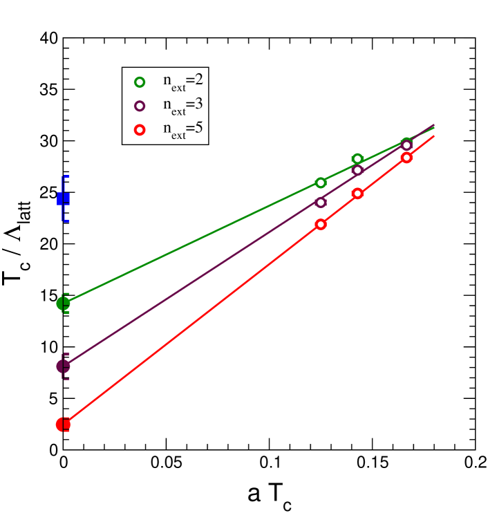
Figure 5: SU(2) in (3+1) dimensions. $T_{c}/\Lambda_{\text{latt}}$ versus $aT_{c}$ for three different values of the external field strength ($n_{\text{ext}}=2,3,5$) on $64^{3}\times L_{t}$ lattices ($L_{t}=6,7,8$). Full points in correspondence of $aT_{c}=0$ are the extrapolations to the continuum. Full square is the critical temperature for SU(2) lattice gauge theory without external field taken from ref. [50].

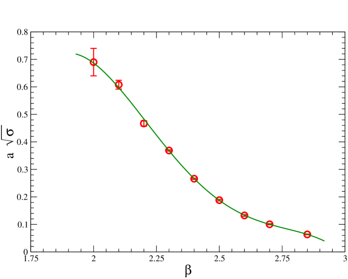
Figure 6: SU(2) string tension in (3+1) dimensions. Open circles are taken from Table 10 of ref. [51]. The solid line is our best fit with Chebyshev polynomials of the first kind up to order 6.

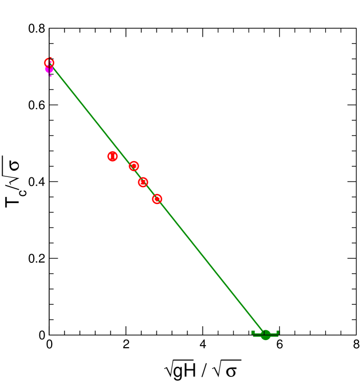
Figure 7: SU(2) in (3+1) dimensions. The critical temperature $T_{c}$ estimated on a $64^{3}\times 8$ lattice in units of the string tension, eq. (25), versus the square root of the field strength $\sqrt{gH}$ in units of the string tension, eq. (26). Solid line is the linear fit eq. (27) On the zero vertical axis are represented the extrapolation of our data to zero value of the field (open circle) and the value for $T_{c}(0)/\sqrt{\sigma}$ (without external field) given in ref. [51] (full circle). The green full circle is the critical field in units of the string tension, eq. (32).

3.2 SU(2)

We also studied the SU(2) lattice gauge theory in a constant abelian chromomagnetic field. Even in this theory the deconfinement temperature turns out to depend on the strength of the applied chromomagnetic field, as already discussed in sect. 1.

We evaluated the critical coupling $\beta^{*}(L_{t},n_{\text{ext}})$ on a $64^{3}\times 8$ lattice versus the strength of the external chromomagnetic field, introduced on the lattice by constraining the links according to eq. (11). As in previous section the critical coupling has been found by locating the peak of the derivative of the free energy density with respect to the gauge coupling $\beta$. Figure 5 shows our analysis for $T_{c}$ in units of $\Lambda_{\text{latt}}$ versus the critical temperature $aT_{c}$ together with a linear extrapolation to the continuum. As one can ascertain there is evidence for a dependence of the critical temperature on the applied field strength. As in the case of SU(3) the critical temperature can be expressed in terms of a physical scale by using a parameterization for the SU(2) string tension obtained by means of a fit to the string tension data collected in Table 10 of ref. [51]. We interpolate the string tension data by using Chebyshev polynomials of the first kind up to order 6 (see fig. 6).

In fig. 7  $T_{c}/\sqrt{\sigma}$ is plotted against $\sqrt{gH}/\sqrt{\sigma}$. As in the SU(3) case discussed in previous section, we can try to fit the data by means of a linear law. Remarkably we found that the linear fit eq. (27) works quite well and we get

$$\frac{T_{c}(0)}{\sqrt{\sigma}}=0.710(13)\qquad\alpha=-0.126(5)\,.$$ (31)

The value obtained for $T_{c}(0)/\sqrt{\sigma}$ is in good agreement with the value $T_{c}/\sqrt{\sigma}=0.694(18)$, without external field, obtained in the literature [51].

Now we can estimate the critical field in string tension units that turns out to be

$$\frac{\sqrt{gH_{c}}}{\sqrt{\sigma}}=5.33\pm 0.33\,.$$ (32)

Note that the critical field $\sqrt{gH_{c}}/\sqrt{\sigma}$ is about a factor 2 greater than the SU(3) critical value in eq. (29). This is at variance of the effective approach within dual superconductor picture in ref. [54], where one gets for the dual critical magnetic field $gH_{c}/\sigma=1$ for SU(2), while $gH_{c}/\sigma=3/4$ for SU(3).

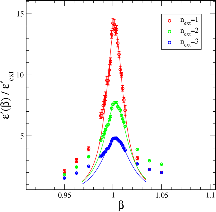
Figure 8: U(1) in (3+1) dimensions. The derivative of the vacuum energy density with respect to $\beta$, eq. (33), versus $\beta$, for several values of the strength of the constant magnetic background field on a $64\times 16^{3}$ lattice. Solid lines are the fits to the data near each of the peaks using eq. (16).

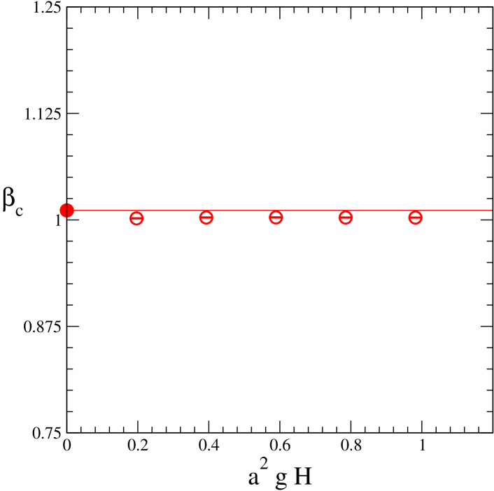
Figure 9: U(1) in (3+1) dimensions. The critical coupling $\beta_{c}$ evaluated on a $64\times 16^{3}$ lattice versus the strength of the constant background magnetic field (in lattice units). The value at zero external field is the infinite volume extrapolation given in ref. [55]. The solid line represents the central value of $\beta_{c}$ from ref. [55].

3.3 U(1)

In sections 3.1 and 3.2 we reported our results indicating a dependence of the deconfinement temperature on the strength of a constant abelian chromomagnetic background field. The main aim of this section is to find out if the effect we found is peculiar of non abelian gauge theories. To this purpose we consider four dimensional U(1) lattice gauge theory.

It is known that, at zero temperature, U(1) lattice gauge theory undergoes a weak first order phase transition [55, 56, 57] from the confined phase to the Coulomb phase for $\beta=1.0111331(21)$ (using the standard Wilson action). We would like to seek a possible dependence of the confinement-Coulomb phase transition on the strength of an applied constant magnetic field.

The quantity we have measured to locate the critical coupling is the derivative of the vacuum energy density (with respect to the gauge coupling) in presence of the background field (see sect. 2)

$$\varepsilon^{\prime}(\beta,n_{\text{ext}})=<U_{\mu\nu}>_{n_{\text{ext}}=0}-<U_{\mu\nu}>_{n_{\text{ext}}\neq 0}\,,$$ (33)

where $<U_{\mu\nu}>_{n_{\text{ext}}}$ is the average plaquette evaluated with $n_{\text{ext}}\neq 0$ and $n_{\text{ext}}=0$ respectively.

In fig. 8 we display the above quantity for three values of the constant abelian background field, normalized to $\varepsilon^{\prime}_{\mathrm{ext}}$, the derivative of the classical energy due to the external applied field

$$\varepsilon^{\prime}_{\mathrm{ext}}=1-\cos(a^{2}gH)=1-\cos(\frac{2\pi}{L_{1}}n_{\mathrm{ext}})\,.$$ (34)

The values of $\beta$ corresponding to the peak in $\varepsilon^{\prime}(\beta,n_{\text{ext}})$ for several values of the strength of the applied constant abelian field are displayed in fig. 9. Our conclusion is that, contrary to non abelian lattice gauge theories, the critical coupling does not depend on the applied magnetic field strength. Analogous result was found in ref. [58] for (2+1)-dimensional compact QED.

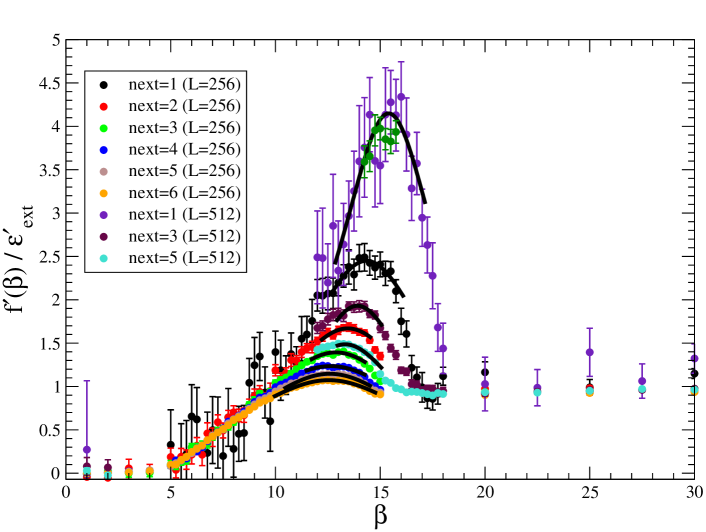
Figure 10: SU(3) in (2+1) dimensions. The derivative of the free energy density with respect to the gauge coupling $\beta$, eq. (14), versus $\beta$ for several values of the external field strength. Lattice size is $L\times 256\times L_{t}$ with two values of $L=256,512$ and temporal lattice size $L_{t}=4$. Solid lines are the fits eq. (16).

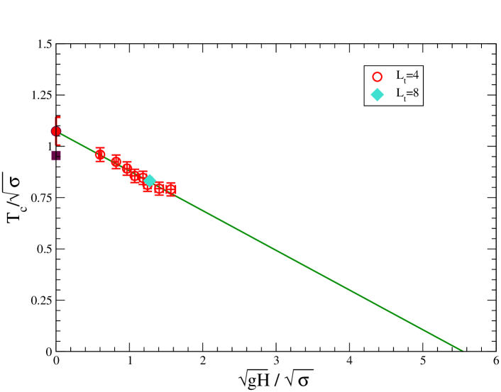
Figure 11: SU(3) in (2+1) dimensions. The critical temperature $T_{c}$ estimated on $256^{2}\times 4$, $512^{2}\times 4$ and $512\times 256\times 8$ lattices in units of the string tension, eq. (25), versus the square root of the field strength $\sqrt{gH}$ in units of the string tension, eq. (26). Open circles refer to $L_{t}=4$, diamond to $L_{t}=8$. Solid line is the linear fit eq. (27). In correspondence of $\sqrt{gH}/\sqrt{\sigma}=0$: full circle represents $T_{c}/\sqrt{\sigma}$ at zero external field obtained by the linear extrapolation eq. (27), full square is the value given in ref. [59].

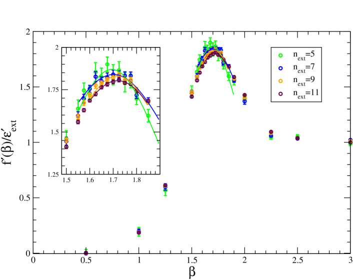
Figure 12: U(1) in (2+1) dimensions. The derivative of the free energy density with respect to $\beta$, eq. (33), versus $\beta$ for several values of the strength of the constant magnetic background field on a $512\times 256\times 4$ lattice. Solid lines are the fits to the data near each of the peaks using eq. (16). The inset is a magnification of the peak region.

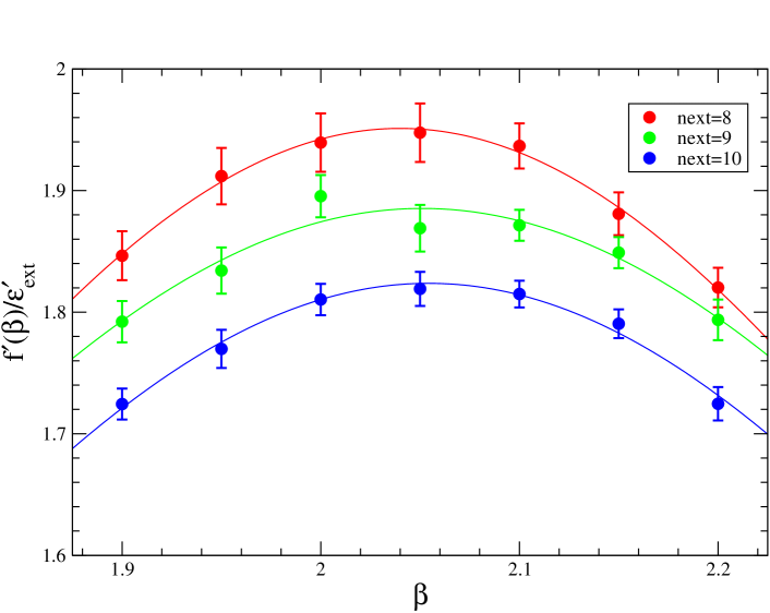
Figure 13: U(1) in (2+1) dimensions. The derivative of the free energy density with respect to $\beta$, eq. (33), versus $\beta$ for several values of the strength of the constant magnetic background field on a $512\times 256\times 8$ lattice. Solid lines are the fits to the data near each of the peaks using eq. (16).

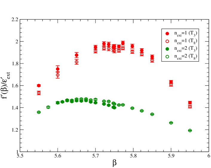
Figure 14: SU(3) in (3+1) dimensions. The derivative of the free energy density with respect to the gauge coupling $\beta$, eq. (14), versus $\beta$ at fixed external field strength ($n_{\text{ext}}=1$) for a $64^{3}\times 8$ lattice. Open symbols refer to $T_{3}$ abelian chromomagnetic field, induced by lattice links in eq. (8). Full symbols refer to $T_{8}$ abelian chromomagnetic field eq. (9).

4 (2+1) dimensions

Our numerical results for non abelian gauge theories SU(2) and SU(3) in (3+1) dimensions in presence of an abelian constant chromomagnetic background field lead us to conclude that the deconfinement temperature depends on the strength of the applied field, and eventually becomes zero for a critical value of the field strength. A natural question arises if this phenomenon, which is peculiar of non abelian gauge theories, continues to hold in (2+1) dimensions. To this purpose we consider here the non abelian SU(3) lattice gauge theory to be contrasted with the abelian U(1) lattice gauge theory at finite temperature.

4.1 SU(3)

In this section we focus on gauge systems in (2+1) dimensions. As is well known gauge theories in (2+1) dimensions possess a dimensionful coupling constant, namely $g^{2}$ has dimension of mass and so provides a physical scale.

Non abelian gauge theories in (2+1) and (3+1) dimensions are sufficiently similar. Indeed, lattice simulations provide convincing evidence that (2+1) dimensional SU(N) gauge theories confine with a linear potential [59]. Moreover, at finite temperature there is a deconfinement transition [60].
In (2+1) dimensions the chromomagnetic field $H^{a}$ is a (pseudo)scalar

$$H^{a}=\frac{1}{2}\varepsilon_{ij}F^{a}_{ij}=F^{a}_{12}\,.$$ (35)

For SU(3) gauge theory a constant abelian chromomagnetic field $H^{3}$ can be obtained with

$$\begin{split}&U^{\mathrm{ext}}_{1}(\vec{x})={\mathbf{1}}\,,\\ &U^{\mathrm{ext}}_{2}(\vec{x})=\begin{bmatrix}\exp(i\frac{gHx_{1}}{2})&0&0\\ 0&\exp(-i\frac{gHx_{1}}{2})&0\\ 0&0&1\end{bmatrix}\end{split}$$ (36)

As in the four dimensional case (see sect. 2.3) since we assume to have a lattice with toroidal geometry the field strength is quantized

$$a^{2}\frac{gH}{2}=\frac{2\pi}{L_{1}}n_{\mathrm{ext}}\,,\qquad n_{\mathrm{ext}}\,\,\,{\text{integer}}\,.$$ (37)

We computed the derivative of the free energy density eq. (5) on a $L\times 256\times 4$ lattice, with $L=256,512$ and several values of the external field strength parameterized by $n_{\text{ext}}$. Our numerical results are reported in fig. 10. We locate the critical coupling $\beta_{c}$ as the position of the maximum of the derivative of the free energy density at given external field strength. As for SU(3) in (3+1) dimensions, the value of $\beta_{c}$ depends on the field strength. Using the parameterization for the string tension given in eq. (C9) of ref. [59]

$$\beta a\sqrt{\sigma}=3.367(50)+\frac{4.1(1.7)}{\beta}+\frac{46.5(11.0)}{\beta^{2}}$$ (38)

we are able to estimate the critical temperature $T_{c}$ in units of the string tension. We find that, as in (3+1) dimensions, $T_{c}/\sqrt{\sigma}$ depends linearly on the applied field strength (see fig. 11). The linear fit eq. (27) gives

$$\frac{T_{c}(0)}{\sqrt{\sigma}}=1.073(87)\quad\alpha=-0.193(76)\,,$$ (39)

that implies a critical field in string tension units $\sqrt{gH_{c}}/\sqrt{\sigma}=5.5\pm 3.7$. Note that value for $T_{c}(0)/\sqrt{\sigma}$ in the present work is in fair agreement with $T_{c}/\sqrt{\sigma}=0.972(10)$ without external field obtained in ref. [60]. To check possible finite volume effects, we performed a lattice simulation with $L_{t}=8$. The result, displayed in fig. 11, shows that within statistical uncertainties our estimate of the critical temperature from the simulation with $L_{t}=8$ is in agreement with result at $L_{t}=4$.

4.2 U(1)

In a classical paper [61] Polyakov showed that compact quantum electrodynamics in (2+1) dimensions at zero temperature confines external charges for all values of the coupling. Moreover it is well ascertained that the confining mechanism is the condensation of magnetic monopoles which gives rise to a linear confining potential and a non-zero string tension

$$\sigma a^{2}=\kappa\frac{1}{\sqrt{\beta}}\exp[-\pi^{2}V(0)\beta]$$ (40)

where $\kappa$ is a constant, $V(0)=0.2527$ [62] is the value of the lattice propagator at zero separation, and $\beta=1/(ag^{2})$.

At finite temperature it is well known that the gauge system undergoes a deconfinement transition which appears to be of the Kosterlitz-Thouless type [63]. We are interested in lattice U(1) gauge theory in an uniform external magnetic field

$$\begin{split}&U^{\text{ext}}_{1}(\vec{x})={\mathbf{1}}\,,\\ &U^{\text{ext}}_{2}(\vec{x})=\cos(gHx_{1})+i\sin(gHx_{1})\,.\end{split}$$ (41)

We performed numerical simulations on $512\times 256\times 4$ and $512\times 64\times 8$ lattices. We measure the derivative of the free energy density with respect to the coupling $\beta$. In fig. 12 we display the results for the $512\times 256\times 4$ lattice. To determine the critical coupling $\beta_{c}$, we fitted the lattice data to eq. (16). Contrary to the case of (2+1) and (3+1) non abelian lattice gauge theories, we do not find a dependence of the critical value of the coupling $\beta_{c}$ on the magnetic field strength. Indeed we found that (temporal size $L_{t}=4$)

$$\begin{split}\beta_{c}(n_{\text{ext}}=5)&=1.694(17)\\ \beta_{c}(n_{\text{ext}}=7)&=1.701(13)\\ \beta_{c}(n_{\text{ext}}=9)&=1.716(11)\\ \beta_{c}(n_{\text{ext}}=11)&=1.719(10))\\ \end{split}$$ (42)

By increasing the temporal size to $L_{t}=8$ the critical coupling increases and is still independent of the external magnetic field strength (see fig. 13). Indeed, we found

$$\begin{split}\beta_{c}(n_{\text{ext}}=8)&=2.040(14)\\ \beta_{c}(n_{\text{ext}}=9)&=2.051(15)\\ \beta_{c}(n_{\text{ext}}=10)&=2.054(12)\\ \end{split}$$ (43)

Therefore we can conclude that even in (2+1) dimensional case the critical coupling does not depend on the strength of the external magnetic field as for U(1) lattice gauge theories in (3+1) dimensions (see sect. 3.3).

5 Conclusions

Let us conclude this paper by stressing our main results. We have investigated U(1), SU(2), and SU(3) pure gauge theories both in (3+1) and (2+1) dimensions in presence of an uniform (chromo)magnetic field. For non abelian gauge theories we found that there is a critical field $gH_{c}$ such that for $gH>gH_{c}$ the gauge systems are in the deconfined phase. Moreover, such an effect seems to be generic for non abelian gauge theories. On the other hand our numerical results for abelian gauge theories, where it is well established [61, 32] that confinement is due to monopole condensation, do not show any dependence of the critical coupling from the strength of an external magnetic field. Therefore it seems very difficult to explain our reversible color Meissner effect in SU(2) and SU(3) gauge theories in terms of abelian color magnetic monopoles. Instead, the peculiar dependence of the deconfinement temperature on the strength of the abelian chromomagnetic field $gH$ could be naturally explained if the vacuum behaved as an ordinary relativistic color superconductor, namely a condensate of color charged scalar fields whose mass is proportional to the inverse of the magnetic length. However, the chromomagnetic condensate cannot be uniform due to gauge invariance of the vacuum, which disorders the gauge system in such a way that there are not long range correlations. Consequently we can speculate that if the vacuum behaved as a non uniform chromomagnetic condensate, our reversible color Meissner effect could be easily explained, for strong enough chromomagnetic fields would force long range color correlations such that the gauge system gets deconfined. One might thus imagine the confining vacuum in non abelian gauge systems as a disordered chromomagnetic condensate which confines color charges due both to the presence of a mass gap and the absence of long range color correlations, as argued by R.P. Feynman in (2+1) dimensions [38].

Appendix A SU(3) $T_{8}$ abelian chromomagnetic background field

As is well known, in SU(3) there are two independent ways to realize a constant abelian chromomagnetic field. The first one, that we have considered in section 3.1, is to take the abelian field directed along direction $\hat{3}$ in color space; the second one is to take the field along direction $\hat{8}$ in color space. In this Appendix we consider SU(3) lattice gauge theory in (3+1) dimensions in presence of a constant chromomagnetic background field along direction $\hat{8}$ in SU(3) color space and along spatial direction $\hat{3}$. The continuum gauge potential and the corresponding lattice links are defined in eq. (7) and eq. (9) respectively. One should not expect a vastly different behavior in the two cases. Indeed we found that, even for a constant abelian chromomagnetic background field directed along color direction $\hat{8}$, the critical deconfinement temperature $T_{c}$ depends on the strength of the applied field. Even more fig. 14, where we display the derivative of the free energy density with respect to the gauge coupling $\beta$ for $n_{\text{ext}}=1,2$ on a $64^{3}\times 8$ lattice, shows that the derivative of the free energy density in presence of the abelian chromomagnetic background field directed along color space direction $\hat{8}$ behaves like the case in which the field is directed along color space direction $\hat{3}$. Moreover the critical couplings at fixed field strength are consistent within statistical errors.

References

- [1] G. ’t Hooft, The confinement phenomenon in quantum field theory, in High Energy Physics, EPS International Conference, Palermo, 1975.
- [2] S. Mandelstam, Vortices and quark confinement in non Abelian gauge theories, Phys. Rept. 23 (1976) 245.
- [3] J. Wosiek and R. W. Haymaker, On the space structure of confining strings, Phys. Rev. D36 (1987) 3297.
- [4] A. Di Giacomo, M. Maggiore, and S. Olejnik, Confinement and chromoelectric flux tubes in lattice QCD, Nucl. Phys. B347 (1990) 441–460.
- [5] P. Cea and L. Cosmai, Lattice investigation of dual superconductor mechanism of confinement, Nucl. Phys. Proc. Suppl. 30 (1993) 572–575.
- [6] V. Singh, D. A. Browne, and R. W. Haymaker, Measurement of the penetration depth and coherence length in U(1) and SU(2) dual abrikosov vortices, Nucl. Phys. Proc. Suppl. 30 (1993) 568–571, [http://arXiv.org/abs/hep-lat/9302010].
- [7] Y. Matsubara, S. Ejiri, and T. Suzuki, The (dual) Meissner effect in SU(2) and SU(3) QCD, Nucl. Phys. Proc. Suppl. 34 (1994) 176–178, [http://arXiv.org/abs/hep-lat/9311061].
- [8] G. S. Bali, K. Schilling, and C. Schlichter, Observing long color flux tubes in SU(2) lattice gauge theory, Phys. Rev. D51 (1995) 5165–5198, [http://arXiv.org/abs/hep-lat/9409005].
- [9] P. Cea and L. Cosmai, Dual Meissner effect and string tension in SU(2) lattice gauge theory, Phys. Lett. B349 (1995) 343–347, [http://arXiv.org/abs/hep-lat/9404017].
- [10] P. Cea and L. Cosmai, Dual superconductivity in the SU(2) pure gauge vacuum: A lattice study, Phys. Rev. D52 (1995) 5152–5164, [http://arXiv.org/abs/hep-lat/9504008].
- [11] A. Di Giacomo, Topological aspects of QCD, Nucl. Phys. Proc. Suppl. 47 (1996) 136–143, [http://arXiv.org/abs/hep-lat/9509036].
- [12] T. Suzuki, K. Ishiguro, Y. Mori, T. Sekido, and I. T. P. Kanazawa U., The dual Meissner effect and Abelian magnetic displacement currents, Phys. Rev. Lett. 94 (2005) 132001, [hep-lat/0410001].
- [13] J. D. Stack and R. J. Wensley, Monopoles, quark confinement and screening in four- dimensional U(1) lattice gauge theory, Nucl. Phys. B371 (1992) 597–617.
- [14] H. Shiba and T. Suzuki, Monopole action and condensation in SU(2) QCD, Phys. Lett. B351 (1995) 519–527, [hep-lat/9408004].
- [15] N. Arasaki, S. Ejiri, S.-i. Kitahara, Y. Matsubara, and T. Suzuki, Monopole action and monopole condensation in SU(3) lattice QCD, Phys. Lett. B395 (1997) 275–282, [hep-lat/9608129].
- [16] N. Nakamura et. al., Disorder parameter of confinement, Nucl. Phys. Proc. Suppl. 53 (1997) 512–514, [hep-lat/9608004].
- [17] M. N. Chernodub, M. I. Polikarpov, and A. I. Veselov, Effective constraint potential for Abelian monopole in SU(2) lattice gauge theory, Phys. Lett. B399 (1997) 267–273, [hep-lat/9610007].
- [18] J. Jersak, T. Neuhaus, and H. Pfeiffer, Scaling analysis of the magnetic monopole mass and condensate in the pure U(1) lattice gauge theory, Phys. Rev. D60 (1999) 054502, [hep-lat/9903034].
- [19] A. Di Giacomo, B. Lucini, L. Montesi, and G. Paffuti, Colour confinement and dual superconductivity of the vacuum. i, Phys. Rev. D61 (2000) 034503, [hep-lat/9906024].
- [20] A. Di Giacomo, B. Lucini, L. Montesi, and G. Paffuti, Colour confinement and dual superconductivity of the vacuum. ii, Phys. Rev. D61 (2000) 034504, [hep-lat/9906025].
- [21] P. Cea and L. Cosmai, Abelian monopole condensation in lattice gauge theories, Nucl. Phys. Proc. Suppl. 83 (2000) 428–430, [hep-lat/9909056].
- [22] C. Hoelbling, C. Rebbi, and V. A. Rubakov, Free energy of an SU(2) monopole-antimonopole pair, Phys. Rev. D63 (2001) 034506, [hep-lat/0003010].
- [23] P. Cea and L. Cosmai, Gauge invariant study of the monopole condensation in non Abelian lattice gauge theories, Phys. Rev. D62 (2000) 094510, [hep-lat/0006007].
- [24] J. M. Carmona, M. D’Elia, A. Di Giacomo, B. Lucini, and G. Paffuti, Color confinement and dual superconductivity of the vacuum. iii, Phys. Rev. D64 (2001) 114507, [hep-lat/0103005].
- [25] J. Greensite, The confinement problem in lattice gauge theory, Prog. Part. Nucl. Phys. 51 (2003) 1, [hep-lat/0301023].
- [26] K. Holland, M. Pepe, and U. J. Wiese, The deconfinement phase transition of Sp(2) and Sp(3) Yang- Mills theories in 2+1 and 3+1 dimensions, Nucl. Phys. B694 (2004) 35–58, [hep-lat/0312022].
- [27] K. Holland, P. Minkowski, M. Pepe, and U. J. Wiese, Exceptional confinement in g(2) gauge theory, Nucl. Phys. B668 (2003) 207–236, [hep-lat/0302023].
- [28] G. Ripka, Dual superconductor models of color confinement, vol. 639 of Lecture Notes in Phys. Springer-Verlag, 2004.
- [29] R. W. Haymaker, Confinement studies in lattice QCD, Phys. Rept. 315 (1999) 153–173, [hep-lat/9809094].
- [30] G. ’t Hooft, Confinement at large N(c), hep-th/0408183.
- [31] P. Cea and L. Cosmai, Abelian monopole and vortex condensation in lattice gauge theories, JHEP 11 (2001) 064.
- [32] E. H. Fradkin and L. Susskind, Order and disorder in gauge systems and magnets, Phys. Rev. D17 (1978) 2637.
- [33] P. Cea and L. Cosmai, Probing the non-perturbative dynamics of SU(2) vacuum, Phys. Rev. D60 (1999) 094506, [hep-lat/9903005].
- [34] P. Cea and L. Cosmai, Abelian chromomagnetic background field at finite temperature on the lattice, http://arXiv.org/abs/hep-lat/0101017.
- [35] P. Cea and L. Cosmai, Abelian chromomagnetic fields and confinement, JHEP 02 (2003) 031, [hep-lat/0204023].
- [36] V. V. Skalozub and A. V. Strelchenko, On generation of Abelian magnetic fields in SU(3) gluodynamics at high temperature, Eur. Phys. J. C33 (2004) 105–112, [hep-ph/0208071].
- [37] M. Tinkham, Introduction to superconductivity. McGraw-Hill, New York, 1975.
- [38] R. P. Feynman, The qualitative behavior of Yang-Mills theory in (2+1)- dimensions, Nucl. Phys. B188 (1981) 479.
- [39] R. Casalbuoni and G. Nardulli, Inhomogeneous superconductivity in condensed matter and QCD, Rev. Mod. Phys. 76 (2004) 263–320, [hep-ph/0305069].
- [40] P. Cea, L. Cosmai, and A. D. Polosa, The lattice Schrödinger functional and the background field effective action, Phys. Lett. B392 (1997) 177–181, [hep-lat/9601010].
- [41] M. Lüscher, R. Narayanan, P. Weisz, and U. Wolff, The Schrödinger functional: A renormalizable probe for non Abelian gauge theories, Nucl. Phys. B384 (1992) 168–228, [hep-lat/9207009].
- [42] M. Lüscher and P. Weisz, Background field technique and renormalization in lattice gauge theory, Nucl. Phys. B452 (1995) 213–233, [hep-lat/9504006].
- [43] G. C. Rossi and M. Testa, The structure of Yang-Mills theories in the temporal gauge. 1. General formulation, Nucl. Phys. B163 (1980) 109.
- [44] D. J. Gross, R. D. Pisarski, and L. G. Yaffe, QCD and instantons at finite temperature, Rev. Mod. Phys. 53 (1981) 43.
- [45] P. Cea, L. Cosmai, and M. D’Elia, The deconfining phase transition in full QCD with two dynamical flavors, JHEP 02 (2004) 018, [hep-lat/0401020].
- [46] P. Cea and L. Cosmai, External fields and color confinement, Nucl. Phys. Proc. Suppl. 140 (2005) 656–658, [http://arXiv.org/abs/hep-lat/0410007].
- [47] A. M. Ferrenberg and R. H. Swendsen, Optimized Monte Carlo analysis, Phys. Rev. Lett. 63 (1989) 1195–1198.
- [48] M. Newman and G. Barkema, Monte Carlo methods in statistical physics. Oxford University Press, New York, 1999.
- [49] A. Davison and D. Hinkley, Bootstrap methods and their application. Cambridge University Press, New York, 1997.
- [50] J. Fingberg, U. Heller, and F. Karsch, Scaling and asymptotic scaling in the SU(2) gauge theory, Nucl. Phys. B392 (1993) 493–517, [hep-lat/9208012].
- [51] M. J. Teper, Glueball masses and other physical properties of SU(N) gauge theories in D = 3+1: a review of lattice results for theorists, hep-th/9812187.
- [52] R. G. Edwards, U. M. Heller, and T. R. Klassen, Accurate scale determinations for the Wilson gauge action, Nucl. Phys. B517 (1998) 377–392, [hep-lat/9711003].
- [53] D. Kabat, K.-M. Lee, and E. Weinberg, QCD vacuum structure in strong magnetic fields, Phys. Rev. D66 (2002) 014004, [hep-ph/0204120].
- [54] M. N. Chernodub, Gluodynamics in external field in dual superconductor approach, Phys. Lett. B549 (2002) 146–153, [hep-ph/0208105].
- [55] G. Arnold, B. Bunk, T. Lippert, and K. Schilling, Compact QED under scrutiny: It’s first order, Nucl. Phys. Proc. Suppl. 119 (2003) 864–866, [hep-lat/0210010].
- [56] M. Vettorazzo and P. de Forcrand, Electromagnetic fluxes, monopoles, and the order of the 4d compact U(1) phase transition, Nucl. Phys. B686 (2004) 85–118, [hep-lat/0311006].
- [57] M. Vettorazzo and P. de Forcrand, Finite temperature phase transition in the 4d compact U(1) lattice gauge theory, Phys. Lett. B604 (2004) 82–90, [hep-lat/0409135].
- [58] M. N. Chernodub, E. M. Ilgenfritz, and A. Schiller, Monopoles, confinement and deconfinement of (2+1)D compact lattice QED in external fields, Phys. Rev. D64 (2001) 114502, [http://arXiv.org/abs/hep-lat/0106021].
- [59] M. J. Teper, SU(N) gauge theories in 2+1 dimensions, Phys. Rev. D59 (1999) 014512, [hep-lat/9804008].
- [60] J. Engels et. al., A study of finite temperature gauge theory in (2+1) dimensions, Nucl. Phys. Proc. Suppl. 53 (1997) 420–422, [hep-lat/9608099].
- [61] A. M. Polyakov, Quark confinement and topology of gauge groups, Nucl. Phys. B120 (1977) 429–458.
- [62] T. Banks, R. Myerson, and J. B. Kogut, Phase transitions in abelian lattice gauge theories, Nucl. Phys. B129 (1977) 493.
- [63] P. D. Coddington, A. J. G. Hey, A. A. Middleton, and J. S. Townsend, The deconfining transition for finite temperature U(1) lattice gauge theory in (2+1)-dimensions, Phys. Lett. B175 (1986) 64.