Color confinement and dual superconductivity of the vacuum. IV.

Abstract

A scaling analysis is made of the order parameter describing monopole condensation at the deconfining transition of $N_{f}=2$ QCD around the chiral point. In accordance with scaling properties of the specific heat, studied in a previous paper, scaling is consistent with a first order transition. The status of dual superconductivity of the vacuum as a mechanism of color confinement is reviewed.

I Introduction

This paper is the fourth of a series PaperI ; PaperII ; PaperIII on a research program aiming at developing and testing on the lattice the working hypothesis that confinement in QCD is produced by dual superconductivity of the vacuum, i.e. by condensation of magnetic charges.

Such a mechanism implies that the deconfining transition is an order–disorder phase transition, i.e. a true phase transition, described by an order parameter.

Another basic underlying idea is duality Kramers:1941kn ; Kadanoff:1970kz : the magnetic excitations which are expected to condense are non local in terms of the fields. They should become local in the dual description, and the strong coupling regime of the confined phase should be mapped by duality in the weak coupling regime for dual fields.

Magnetic charges exist in gauge theories Dirac:1931kp ; 'tHooft:1974qc ; Polyakov:1974ek and are nicely described in a formulation of the theory based on parallel transport, as the Wilson formulation is  Wilson:1974sk .

The prototype theory is the lattice $U(1)$ gauge theory in 4d. In the Wilson’s formulation this theory shows a deconfining transition at $\beta\equiv 2/g^{2}\simeq 1.01$, from a strong coupling phase in which static charges are confined, to a Coulomb phase. Dual magnetic excitations can be defined and with them an order parameter which is the vev $\langle\mu\rangle$ of a magnetically charged operator $\mu$. This vev is different from zero in the confined phase, and strictly zero in the deconfined phase. This operator is defined by its correlation functions Frohlich:1986sz ; Frohlich:1987er ; Frohlich:1982gf , exactly like the kink’s correlators in the Ising model of Ref. Kadanoff:1970kz . It can however be explicitly defined as a non local operator in terms of the gauge fields Marino:1981we ; DiGiacomo:1997sm in the same way as the kink creation operator can be explicitly written in terms of the spin variables Carmona:2000eu .

The operator $\mu$ is a gauge invariant Dirac like Frohlich:1986sz ; Frohlich:1987er ; Frohlich:1982gf magnetic charged operator, non local but obeying cluster property, and a rigorous proof exists that it is the correct order parameter, both for the Villain Frohlich:1987er and for the Wilson Cirigliano:1997zq actions. In the presence of electric charges, however, there are problems for the existence of the duality transformation Frohlich:2000zp . We will come back below in Sect. II.

The translation of the above formalism into non abelian gauge theories is non trivial. The original proposal to define and expose monopoles 'tHooft:1981ht is based on a procedure known as abelian projection. A gauge is fixed, e.g. by diagonalizing any observable in the adjoint representation, a residual $U(1)^{N-1}$ gauge invariance is left and the monopoles are defined as monopoles of each of these $U(1)$s, as for the abelian case. They show up as singularities of the gauge transformation which brings to the abelian projected gauge, in the sites in which two eigenvalues of the chosen observable coincide.

In this way the number and the location of monopoles in a given field configuration depends on the abelian projection, i.e. on the choice of the gauge, and there is a functional infinity of ways to do it.

Therefore if one pretends that the monopoles detected on the lattice configurations are the relevant degrees of freedom for confinement (monopole dominance Suzuki:1989gp ), then one has to select the abelian projection which defines them. The usual choice is the so called maximum abelian projection, by which a gauge is selected maximizing the role of the residual abelian degrees of freedom. In some literature this choice is called the abelian projection tout-court. According to this approach the monopoles in this projection are the effective degrees of freedom for confinement.

An alternative attitude is to look at the change of symmetries at the transition, postponing the identification of the relevant excitations, which is a far more difficult problem. This amounts to define and test an order parameter $\langle\mu\rangle$ for monopole condensate.

The lattice version of the operator $\mu$ has been constructed in I, II. $\mu(\vec{x},t)$ creates a monopole in a given abelian projection at the site $(\vec{x},t)$. $\mu$ is color gauge invariant, magnetic $U(1)$ gauge invariant Frohlich:1982gf , but of course is abelian projection dependent.

In III it was shown numerically that the order parameter $\langle\mu\rangle$ is abelian projection independent. Arguments were given in Ref. DiGiacomo:2002pe justifying theoretically this observation. Below we will present a complete argument showing that the statement $\langle\mu\rangle\neq 0$ or $\langle\mu\rangle=0$ is abelian projection independent. Any $\mu$ creates a monopole in all abelian projections. The recent observation of the existence of abelian Abrikosov flux tubes even without fixing the gauge fully supports this view Suzuki:2004uz .

Creating a monopole is a better defined operation than detecting it; the same is true also for $Z_{n}$ vortices vort1 . Their creation is gauge independent; their detection depends on the choice of the gauge.

In summary $\langle\mu\rangle$ proves to be a good order parameter for the quenched theory: it is gauge invariant, abelian projection independent, strictly zero in the deconfined phase in the infinite volume limit PaperI ; PaperII ; D'Elia:2003xn , non zero in the confined phase and its scaling with volume is consistent with the critical indexes of the transition.

On this basis $\langle\mu\rangle$ can be tentatively used as an order parameter for confinement also in full QCD. This would fill a gap: indeed in full QCD no $Z_{3}$ symmetry exists, the chiral phase transition is defined at $m_{q}=0$, but an order parameter for confinement is missing.

In Ref. Carmona:2002ty ; Carmona:2002ye ; Carmona:2002yg it was proved numerically that, for $N_{f}=2$, $\langle\mu\rangle\neq 0$ below the “transition line” and $\langle\mu\rangle=0$ above it. In this paper we discuss a finite size scaling analysis of the order parameter for $N_{f}=2$ QCD. We find that it is consistent with a first order phase transition. The same indication comes from the analysis of the specific heat and of the chiral order parameter at the chiral transition CHIPAPER .

In Sect. II we review the status of the order parameter $\langle\mu\rangle$: its independence on the abelian projection, the difficulties related to the coexistence in the theory of electric and magnetic charges.

In Sect. III we present the numerical results for $N_{f}=2$ QCD and a scling analysis of the order of the deconfinement phase transition.

Sect. IV contains the conclusions and perspectives.

II The (dis)order parameter $\langle\mu\rangle$

The operator $\mu^{a}$ ($a=1,\ldots,N_{c}-1$) which creates a monopole of the species $a$ in a given abelian projection is defined in the continuum as DiGiacomo:2003ee

$$\mu^{a}(\vec{x},t)=\\ \exp\left[i\int\!\!d\vec{y}\,\,{\rm Tr}\{\phi^{a}(\vec{y},t)\vec{E}(\vec{y},t)\}\vec{b}_{\perp}(\vec{x}-\vec{y})\right]\,.$$ (1)

Here

• $\vec{b}_{\perp}(\vec{x}-\vec{y})$ is the vector potential produced by a Dirac $U(1)$ monopole sitting at $\vec{x}$ in the transverse gauge:

  $$\vec{\nabla}\cdot\vec{b}_{\perp}=0\;\;;\;\;\vec{\nabla}\wedge\vec{b}_{\perp}(\vec{r})=\frac{2\pi}{g}\frac{\vec{r}}{r^{3}}+\text{Dirac String}\,;$$

• $\phi^{a}$ transforms in the adjoint representation and has the form

  $$\phi^{a}(x)=U^{\dagger}(x)\phi^{a}_{diag}U(x)$$ (2)

  with

  $$\phi^{a}_{diag}=\mathrm{diag}\,\Big{(}\overbrace{\frac{N_{c}-a}{N_{c}},\ldots,\frac{N_{c}-a}{N_{c}}}^{a},\overbrace{-\frac{\vphantom{N_{c}}a}{N_{c}},\ldots,-\frac{a}{N_{c}}}^{N_{c}-a}\Big{)}\,.$$

  The gauge transformation $U$ identifies the representation in which $\phi^{a}(x)$ is diagonal, i.e. the abelian projection. Of course $\mu^{a}$ depends on $U$, i.e. on the abelian projection.

In the abelian projected gauge $\phi^{a}=\phi^{a}_{diag}$, which is $x$ independent, the longitudinal part of $\vec{E}$ in Eq. 1 cancels in the convolution with $\vec{b}_{\perp}$, and only the diagonal part of $\vec{E}$ contributes to the trace on color indexes. If we define the matrices $T^{a}$ ($a=1,\ldots,N_{c}-1$) as

$$T^{a}\equiv\mathrm{diag}\big{(}\underbrace{0,\ldots,0,\overset{a}{1},\overset{a+1}{-1},0,\dots,0}_{N_{c}}\big{)}$$

these matrices are a complete basis for traceless diagonal matrices. Therefore

$$\vec{E}_{\perp\,\,diag}=\sum\vec{E}^{a}_{\perp\,\,diag}T^{a}$$

and since

$${\rm Tr}\{\phi^{a}_{diag}T^{b}\}=\delta^{ab}$$

in the abelian projected gauge

$$\mu^{a}(\vec{x},t)=\exp\left[i\int\!\!d\vec{y}\,\,\vec{E}^{a}_{\perp\,\,diag}(\vec{y},t)\vec{b}_{\perp}(\vec{x}-\vec{y})\right]\,.$$

$\vec{E}^{a}_{\perp\,\,diag}$ is the conjugate momentum to $\vec{A}^{a}_{\perp}$, so that in the Schrödinger representation

$$\mu^{a}(\vec{x},t)\,\,\lvert\vec{A}^{a}_{\perp}(\vec{x},t)\rangle=\lvert\vec{A}^{a}_{\perp}(\vec{x},t)+\vec{b}_{\perp}(\vec{x}-\vec{y})\rangle$$

$\mu^{a}$ creates a Dirac monopole in the residual $U(1)$ gauge field in the direction of $T^{a}$.

On the other hand it can be proved 'tHooft:1981ht ; PaperI ; PaperII that the ’t Hooft tensor corresponding to a scalar field $\phi$ in the adjoint representation

$$F_{\mu\nu}\equiv{\rm Tr}\left\{\phi G_{\mu\nu}-\frac{i}{g}\phi\left[D_{\mu}\phi,D_{\nu}\phi\right]\right\}$$ (3)

reduces to an abelian form if and only if $\phi$ has the form $\phi^{a}$ of Eq. 2. In that case indeed Eq. 3 becomes

$$F^{a}_{\mu\nu}(x)={\rm Tr}\left\{\partial_{\mu}(\phi^{a}A_{\nu})-\partial_{\nu}(\phi^{a}A_{\mu})-\frac{i}{g}\phi^{a}\left[\partial_{\mu}\phi^{a},\partial_{\nu}\phi^{a}\right]\right\}\,;$$

the quadratic terms in $A_{\mu}A_{\nu}$ in the definition of $F_{\mu\nu}$ cancel and

$$\partial_{\mu}F^{\star a}_{\mu\nu}\equiv\partial_{\mu}\left(\frac{1}{2}\epsilon_{\mu\nu\rho\sigma}F^{a}_{\rho\sigma}\right)=0\,,$$

i.e. the Bianchi identities are obeyed except for singularities. In the abelian projected gauge $\partial_{\mu}\phi^{a}=0$, $(A_{\mu})_{diag}=\sum A_{\mu}^{a}T^{a}$ and

$$F^{a}_{\mu\nu}=\partial_{\mu}A^{a}_{\nu}-\partial_{\nu}A^{a}_{\mu}\,.$$

For the simple case of $SU(2)$ $a$ only assumes the value $a=1$,

$$\phi^{1}_{diag}=\frac{1}{2}\begin{pmatrix}1&0\\ 0&-1\end{pmatrix}=\frac{1}{2}\sigma_{3}\;\;;\;\;\phi^{1}(x)=U^{\dagger}(x)\frac{1}{2}\sigma_{3}U(x)\,.$$

For $SU(2)$ any hermitian field $\phi(x)$ in the adjoint representation can be put in the form $\phi(x)=U^{\dagger}(x)\frac{1}{2}\sigma_{3}U(x)$; meaning that an abelian projection is obtained by diagonalizing $\phi(x)$. Monopoles will appear when the gauge transformation $U(x)$ is singular, and this happens when $|\phi(x)|=0$, i.e. when two eigenvalues of $\phi(x)$ coincide 'tHooft:1981ht .

For generic $SU(N)$ any hermitian field $\phi(x)$ in the adjoint representation can be written as

$$\phi(x)=\sum c_{a}(x)U^{\dagger}(x)\phi^{a}_{diag}U(x)$$

with $U(x)$ the gauge transformation which diagonalizes $\phi(x)$ and orders the eigenvalues (for instance in a decreasing order for their imaginary parts). $U(x)$ will be singular at points where any of the coefficients $c_{a}(x)$ is zero. In these points two eigenvalues of $\phi$ coincide. Indeed from the definition of $\phi^{a}(x)$, in the abelian projected gauge $\phi^{a}=\phi^{a}_{diag}$ and $\phi_{ii}(x)-\phi_{(i+1)(i+1)}(x)=c_{i}(x)$. The matrices $\phi^{a}_{diag}$ play in $SU(N)$ the analogous role as $\sigma_{3}/2$ in $SU(2)$.

One can define magnetic currents

$$j^{a}_{\mu}(x)\equiv\partial_{\mu}F^{\star a}_{\mu\nu}\,.$$

Those currents are zero everywhere, because of Bianchi identities, except at singular points where monopoles are located. In any case

$$\partial_{\mu}j^{a}_{\mu}=0$$

defining a magnetic $U(1)$ symmetry, and conservation of magnetic charge. If this symmetry is realized à la Wigner, i.e. if the vacuum has definite magnetic charge, the system is normal. The vacuum is a magnetic superconductor if it does not have a definite magnetic charge, but is a superposition of states with different magnetic charges. $\langle\mu^{a}\rangle\neq 0$ can signal the second possibility. In the normal state $\langle\mu^{a}\rangle=0$

The lattice version of $\mu^{a}$ has been constructed in I and II, and is equally well defined in the presence of dynamical quarks. It was numerically shown in III that being $\langle\mu^{a}\rangle=0$ or $\langle\mu^{a}\rangle\neq 0$ is a property independent of the choice of the abelian projection, and is shared by the version in which $\phi^{a}$ is put diagonal configuration by configuration, which is kind of an average on infinitely many abelian projections. The same thing results from comparison of measurements of $\langle\mu^{a}\rangle$ in different abelian projections with measurement made by use of Scrödinger functional Cea:1996ff as in Ref. Cea:2001an . More recently flux tubes were observed in $SU(2)$ gauge configurations in the $\sigma_{3}$ direction without fixing the abelian projection Suzuki:2004uz .

In fact, if the density of monopoles is finite, i.e. if in whatever abelian projection there exists a finite number of them per unit volume, then the gauge transformation $V(x)$ which connects two abelian projections is continuos everywhere except at a finite number of points, where monopoles are located.

Creating a monopole with $\mu^{a}(x)$ will add a singularity say in one of the abelian projections: the probability that $x$ coincides with the position of a monopole already present will be zero, and there will be a neighbourhood of $x$ in which $V$ is regular. Adding a singularity in one of the abelian projections amounts to add a new singularity also in the others. $\mu^{a}$ creates a monopole in all abelian projections. Therefore $\langle\mu^{a}\rangle\neq 0$ means Higgs breaking of magnetic charge of type “$a$” in all of them.

Dual superconductivity is an absolute property, independent of the abelian projection.

The density of monopoles is known to be finite Bornyakov:2003kn . A direct test of that can be made by looking at the distribution of the difference between eigenvalues of any hermitian operator in the adjoint representation. Finding, in any site of the lattice, a zero difference would mean that a monopole is sitting on the site. The lattice can be made finer and finer by increasing $\beta$. Fig. 1 shows that in no site the eigenvalues coincide, and hence that the density of monopoles is finite. The same happens at higher values of $\beta$.

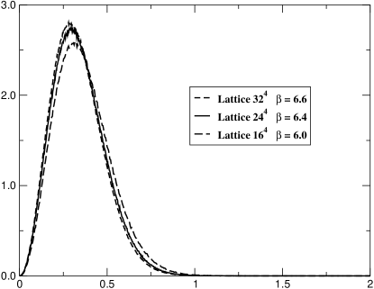
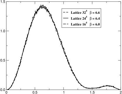
Figure 1: Normalized distribution of the difference between the phases of consecutive eigenvalues (in units of $\pi$) of the plaquette operator (upper figure) and of the Polyakov loop (lower figure). The values $0$ or $2$ correspond to two coincident eigenvalues and thus to the presence of monopoles. The distribution has been measured at different values of $\beta$ and approximately equal physical volumes, in order to check the continuum limit.

A last point concerns the problem raised in Ref. Frohlich:2000zp about the difficulty to obey Dirac condition for magnetic charges in the presence of electric charges. This is a general problem: in $U(1)$ this difficulty shows up as the non existence of the duality transformation, and this produces problems at short distances: an operator like $\mu$ should be modified at distances $\mathcal{O}(a)$ by terms $\mathcal{O}(a^{2})$. The authors of Ref. Frohlich:2000zp suggest a modified formulation in which a coulombic magnetic field produced by a monopole is replaced by a superposition of radial flux tubes with quantized flux Chernodub:2000wk . This is a big revision in the description of a monopole, but is in any case unmanageable from the numerical point of view Belavin:2002hb . In any case our operator is defined up to term $\mathcal{O}(a^{2})$ as explained in I Sect. II, so that looking for $\mathcal{O}(a^{2})$ corrections would be meaningless anyhow. Contrary to $U(1)$ $\mathcal{O}(a^{2})$ corrections in QCD should become unimportant in the continuum limit because of asymptotic freedom. The problem is however open and deserves further investigation.

III $N_{f}=2$ QCD

The study of the QCD finite temperature transition for 2 flavors is of fundamental importance. The phase transition is well understood at high masses ($m\geq 2.5$ $GeV$), where the quarks decouple; the transition is first order and the Polyakov line is a good order parameter. At $m\simeq 0$ a chiral transition exists, where chiral symmetry is restored, and the chiral condensate $\langle\bar{\psi}\psi\rangle$ is an order parameter. At some temperature also the axial $U_{A}(1)$ is expected to be restored: indeed the topological susceptibility drops to zero around $T_{c}$ Alles:2000cg . In principle at $m\simeq 0$ there are 3 transitions (chiral, axial $U_{A}(1)$, deconfinement): it is not clear if they coincide. An effective description of the chiral transition can be given in terms of an effective free energy Pisarski:1983ms . Assuming that the scalar and pseudoscalar modes are the relevant critical degrees of freedom, there is no infrared stable fixed points for $N_{f}\geq 3$ and the transition is expected to be first order. For $N_{f}=2$ the transition is first order if the anomaly is negligible ($m_{\eta^{\prime}}\approx 0$) at $T_{c}$; it can be second order with symmetry $O(4)$ if the anomaly survives the chiral transition. In the first case the transition surface around $m=0$ is first order. If the chiral transition is instead second order the surface is a crossover, and a tricritical point is expected in the $\mu-T$ plane (see e.g. Stephanov:1998dy ), detectable by heavy ion experiments.

The first scenario is compatible with dual superconductivity of the vacuum being the mechanism for confinement both in pure gauge and in presence of dynamical quarks, independently of their mass: the deconfinement transition is then always an order-disorder phase transition, not a crossover. If the second is the case instead, the deconfining transition cannot be order-disorder, there is no order parameter for confinement, and a state of a free quark can continuously be transfered below the “deconfining temperature”: confined and deconfined then lose a definite meaning.

The question can be answered by a numerical study of the chiral phase transition and has been the subject of extensive, even if not conclusive, literature Fukugita:1990vu ; Fukugita:1990dv ; Brown:1990ev ; Karsch:1993tv ; Karsch:1994hm ; Bernard:1999fv ; AliKhan:2000iz . In Ref. CHIPAPER we have presented a large scale finite size scaling analysis of the 2 flavor chiral transition by looking at the specific heat, the chiral susceptibilty and the equation of state: we have found clear disagreement with a second order $O(4)$ behaviour and solid indications of the possible presence of a first order phase transition. On the other hand the fact that dual superconductivity is at work also in the presence of two dynamical flavours has been already shown, for finite quark masses ($m_{\pi}/m_{\rho}\simeq 0.505$), in Ref. Carmona:2002yg , using $\langle\mu\rangle$ as a disorder parameter, and also in the Schrödinger functional approach in Ref. Cea:2004ux .

In this Section we present a finite size scaling analysis of $\langle\mu\rangle$ around the chiral phase transition: if $\langle\mu\rangle$ is the correct (dis)order parameter for confinement, this analysis will give the correct critical indexes.

The parameter $\langle\mu\rangle$ is defined on the lattice as (see I and II)

$$\langle\mu\rangle=\frac{\tilde{Z}}{Z}\;,$$

$$Z=\int\left({\cal D}U\right)e^{-\beta S}\;,$$

$$\tilde{Z}=\int\left({\cal D}U\right)e^{-\beta\tilde{S}}\;.$$ (4)

$\tilde{Z}$ is obtained from $Z$ by changing the action in the time slice $x_{0}$, $S\to\tilde{S}=S+\Delta S$. In the Abelian projected gauge the plaquettes

$$\Pi_{i0}(\vec{x},x_{0})=$$

$$=U_{i}(\vec{x},x_{0})U_{0}(\vec{x}+\hat{\imath},x_{0})U_{i}^{\dagger}(\vec{x},x_{0}+\hat{0})U_{0}^{\dagger}(\vec{x},x_{0})$$ (5)

are changed by substituting

$$U_{i}(\vec{x},x_{0})\to\tilde{U}_{i}(\vec{x},x_{0})\equiv U_{i}(\vec{x},x_{0})e^{iTb^{i}_{\perp}(\vec{x}-\vec{y})}$$ (6)

where $T$ is the diagonal gauge group generator corresponding to the monopole species chosen. The numerical determination of $\langle\mu\rangle$ is very difficult, since $\langle\mu\rangle$ is expressed as the ratio of two partition functions. Instead of $\langle\mu\rangle$ we measure the quantity

$$\rho=\frac{d}{d\beta}\ln\langle\mu\rangle\;.$$ (7)

It follows from Eq. (III) that

$$\rho=\langle S\rangle_{S}-\langle\tilde{S}\rangle_{\tilde{S}}\;,$$ (8)

the subscript meaning the action by which the average is performed. In terms of $\rho$

$$\langle\mu\rangle=\exp\left(\int_{0}^{\beta}\rho(\beta^{\prime})\mbox{d}\beta^{\prime}\right)\;.$$ (9)

A drop of $\langle\mu\rangle$ at the phase transition corresponds to a strong negative peak of $\rho$. A negative value of $\rho$ diverging in the thermodynamical limit in the deconfined phase means $\langle\mu\rangle$ being exactly zero on that side (see I, II, III).

We have made simulations with two degenerate flavors of Kogut-Susskind quarks, using the standard gauge and fermion actions. Configuration updating was performed using the standard Hybrid R algorithm Gottlieb:1987mq . The lattice temporal size was fixed at $N_{t}=4$. Different spatial sizes ($L=12,16,20,24,32$) and values of the quark mass were used. For a more detailed account on simulation parameters we refer to CHIPAPER .

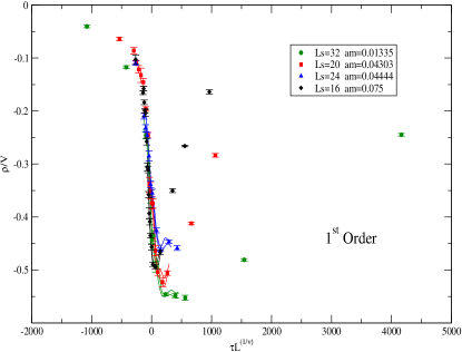
Figure 2: Finite size scaling of $\rho$ according to the critical indexes of first order transition.

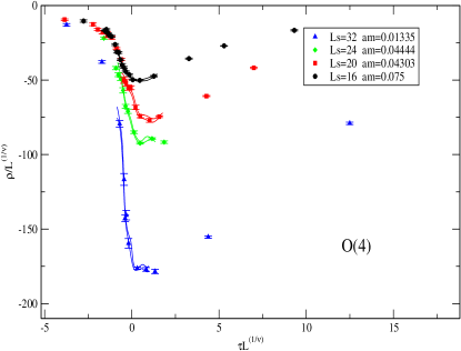
Figure 3: Finite size scaling of $\rho$ according to the $O(4)$ critical indexes.

We can assume the following general scaling form for $\langle\mu\rangle$ around the phase transition:

$$\langle\mu\rangle=L^{k}\Phi(\tau L^{1/\nu},mL^{y_{h}})$$

where $\tau$ is the reduced temperature and $m$ the quark mass. Sending $L$ to infinity keeping $\xi/L$ or $\tau L^{1/\nu}$ fixed, must be a convergent limit. Analyticity arguments D'Elia:2004xi ; Karsch:1994hm suggest that in the infinite volume limit the mass dependence in the scaling function factorizes, so that $\rho=\frac{d}{d\beta}\ln\langle\mu\rangle$ does not depend on the mass. In fact, the dependence on $mL^{y_{h}}$ must then cancel the dependence on the factor $L^{k}$ in front. We then obtain the following scaling law:

$$\rho=L^{1/\nu}\phi(\tau L^{1/\nu})\;.$$ (10)

the same as in the quenched case.

In Figure 2 we show the quality of scaling assuming $\nu=1/3$, i.e. a first order phase transition: a good agreement is clearly visible. The deviations from scaling in the deconfined region are expected D'Elia:2003xn and are related to the disorder parameter $\langle\mu\rangle$ being exactly zero on that side.

For comparison we show in Figure 3 the quality of scaling assuming the $O(4)$ critical index $\nu=0.75$.

The $O(4)$ universality class is clearly excluded, while there is good agreement with a first order phase transition. This confirms results obtained through an analysis of the specific heat and of the chiral susceptibility CHIPAPER .

IV Conclusions

QCD with $N_{f}=2$ is a specially interesting system to investigate confinement. The order of the chiral phase transition can indeed decide if the deconfining transition is a real transition, as required by a mechanism of confinement like dual superconductivity, or a trivial cross-over.

More generally the very possibility of defining confined versus deconfined relies on the existence of an order parameter. This parameter exists for the quenched theory, where the transition is first order, but is not defined for full QCD. For full QCD only a chiral order parameter $\langle\bar{\psi}\psi\rangle$ is defined, and only at low enough quark masses.

We have shown that an order parameter $\langle\mu\rangle$ can be defined, which, independently of the presence of quarks and of their masses, characterizes confinement and deconfinement. $\langle\mu\rangle\neq 0$ at $T<T_{c}$; $\langle\mu\rangle$ strictly zero in the limit $V\rightarrow\infty$ for $T>T_{c}$.

A finite size scaling analysis gives the correct (pseudo)critical indexes both for the quenched and for the $N_{f}=2$ case. For $N_{f}=2$ the deconfining transition as seen by looking at $\langle\mu\rangle$ is first order. This is the main result of the present article. The same indication comes from the analysis of the specific heat CHIPAPER , which is independent of any prejudice on the mechanism of confinement.

Further study is on the way with improved actions and algorithm to settle this issue, as well as to study the behavior of $m_{\eta^{\prime}}$ at the chiral transition point.

A consistent picture starts to emerge for confinement. A theoretical problem in the definition of $\langle\mu\rangle$ in the presence of electric charges exists, which deserves further study.

- (1) A. Di Giacomo, B. Lucini, L. Montesi and G. Paffuti, Phys. Rev. D 61 (2000) 034503 [arXiv:hep-lat/9906024].
- (2) A. Di Giacomo, B. Lucini, L. Montesi and G. Paffuti, Phys. Rev. D 61 (2000) 034504 [arXiv:hep-lat/9906025].
- (3) J. M. Carmona, M. D’Elia, A. Di Giacomo, B. Lucini and G. Paffuti, Phys. Rev. D 64 (2001) 114507 [arXiv:hep-lat/0103005].
- (4) H. A. Kramers and G. H. Wannier, Phys. Rev. 60 (1941) 252.
- (5) L. P. Kadanoff and H. Ceva, Phys. Rev. B 3 (1971) 3918.
- (6) P. A. M. Dirac, Proc. Roy. Soc. Lond. A 133 (1931) 60.
- (7) G. ’t Hooft, Nucl. Phys. B 79 (1974) 276.
- (8) A. M. Polyakov, JETP Lett. 20 (1974) 194 [Pisma Zh. Eksp. Teor. Fiz. 20 (1974) 430].
- (9) K. G. Wilson, Phys. Rev. D 10 (1974) 2445.
- (10) J. Frohlich and P. A. Marchetti, Europhys. Lett. 2 (1986) 933.
- (11) J. Frohlich and P. A. Marchetti, Commun. Math. Phys. 112 (1987) 343.
- (12) J. Frohlich and T. Spencer, Commun. Math. Phys. 83 (1982) 411.
- (13) E. C. Marino, B. Schroer and J. A. Swieca, Nucl. Phys. B 200 (1982) 473.
- (14) A. Di Giacomo and G. Paffuti, Phys. Rev. D 56 (1997) 6816 [arXiv:hep-lat/9707003].
- (15) J. M. Carmona, A. Di Giacomo and B. Lucini, Phys. Lett. B 485 (2000) 126 [arXiv:hep-lat/0005014].
- (16) V. Cirigliano and G. Paffuti, Commun. Math. Phys. 200 (1999) 381 [arXiv:hep-th/9707219].
- (17) J. Frohlich and P. A. Marchetti, Phys. Rev. D 64 (2001) 014505 [arXiv:hep-th/0011246].
- (18) G. ’t Hooft, Nucl. Phys. B 190, 455 (1981).
- (19) T. Suzuki and I. Yotsuyanagi, Phys. Rev. D 42 (1990) 4257.
- (20) A. Di Giacomo, arXiv:hep-lat/0206018.
- (21) T. Suzuki, K. Ishiguro, Y. Mori and T. Sekido, arXiv:hep-lat/0410039.
- (22) L. Del Debbio, A. Di Giacomo, B. Lucini, Nucl. Phys. B594, 287 (2001).
- (23) M. D’Elia, A. Di Giacomo and B. Lucini, Phys. Rev. D 69 (2004) 077504 [arXiv:hep-lat/0309004].
- (24) J. M. Carmona, M. D’Elia, L. Del Debbio, A. Di Giacomo, B. Lucini and G. Paffuti, Phys. Rev. D 66 (2002) 011503 [arXiv:hep-lat/0205025].
- (25) J. M. Carmona, M. D’Elia, L. Del Debbio, A. Di Giacomo, B. Lucini, G. Paffuti and C. Pica, Nucl. Phys. A 715 (2003) 883 [arXiv:hep-lat/0209080].
- (26) J. M. Carmona, M. D’Elia, L. Del Debbio, A. Di Giacomo, B. Lucini, G. Paffuti and C. Pica, Nucl. Phys. Proc. Suppl. 119 (2003) 697 [arXiv:hep-lat/0209082].
- (27) M. D’Elia, A. Di Giacomo and C. Pica, [arXiv:hep-lat/0503030]
- (28) A. Di Giacomo and G. Paffuti, Nucl. Phys. Proc. Suppl. 129 (2004) 647 [arXiv:hep-lat/0309019].
- (29) P. Cea, L. Cosmai and A. D. Polosa, Phys. Lett. B 392 (1997) 177 [arXiv:hep-lat/9601010].
- (30) P. Cea and L. Cosmai, JHEP 0111 (2001) 064.
- (31) V. G. Bornyakov, P. Y. Boyko, M. I. Polikarpov and V. I. Zakharov, Nucl. Phys. B 672 (2003) 222 [arXiv:hep-lat/0305021].
- (32) M. N. Chernodub, F. V. Gubarev, M. I. Polikarpov and V. I. Zakharov, Nucl. Phys. B 592 (2001) 107 [arXiv:hep-th/0003138].
- (33) V. A. Belavin, M. N. Chernodub and M. I. Polikarpov, Nucl. Phys. Proc. Suppl. 106 (2002) 610 [arXiv:hep-lat/0110150].
- (34) B. Alles, M. D’Elia and A. Di Giacomo, Phys. Lett. B 483 (2000) 139 [arXiv:hep-lat/0004020].
- (35) R. D. Pisarski and F. Wilczek, Phys. Rev. D 29 (1984) 338.
- (36) M. A. Stephanov, K. Rajagopal and E. V. Shuryak, Phys. Rev. Lett. 81 (1998) 4816 [arXiv:hep-ph/9806219].
- (37) M. Fukugita, H. Mino, M. Okawa and A. Ukawa, Phys. Rev. Lett. 65 (1990) 816.
- (38) M. Fukugita, H. Mino, M. Okawa and A. Ukawa, Phys. Rev. D 42 (1990) 2936.
- (39) F. R. Brown et al., Phys. Rev. Lett. 65 (1990) 2491.
- (40) F. Karsch, Phys. Rev. D 49 (1994) 3791 [arXiv:hep-lat/9309022].
- (41) F. Karsch and E. Laermann, Phys. Rev. D 50 (1994) 6954 [arXiv:hep-lat/9406008].
- (42) C. W. Bernard et al., Phys. Rev. D 61 (2000) 054503 [arXiv:hep-lat/9908008].
- (43) A. Ali Khan et al. [CP-PACS Collaboration], Phys. Rev. D 63 (2001) 034502 [arXiv:hep-lat/0008011].
- (44) P. Cea, L. Cosmai and M. D’Elia, JHEP 0402 (2004) 018 [arXiv:hep-lat/0401020].
- (45) S. A. Gottlieb, W. Liu, D. Toussaint, R. L. Renken and R. L. Sugar, Phys. Rev. D 35 (1987) 2531.
- (46) M. D’Elia, A. Di Giacomo and C. Pica, arXiv:hep-lat/0408011.