Two flavor QCD and Confinement

Abstract

We argue that the order of the chiral transition for $N_{f}=2$ is a sensitive probe of the QCD vacuum, in particular of the mechanism of color confinement. A strategy is developed to investigate the order of the transition by use of finite size scaling analysis. An in-depth numerical investigation is performed with staggered fermions on lattices with $N_{t}=4$ and $N_{s}=12,16,20,24,32$ and quark masses $am_{q}$ ranging from 0.01335 to 0.307036. The specific heat and a number of susceptibilities are measured and compared with the expectations of an $O(4)$ second order and of a first order phase transition. A second order transition in the $O(4)$ and $O(2)$ universality classes are excluded. Substantial evidence emerges for a first order transition. A detailed comparison with previous works is performed.

I Introduction

$N_{f}=2$ QCD can provide fundamental insight into the mechanism of confinement. A schematic view of the phase diagram is shown in Fig. 1 Review . The quark masses are assumed to be equal for the sake of simplicity: $m_{u}=m_{d}=m$; $\mu$ is the baryon chemical potential.

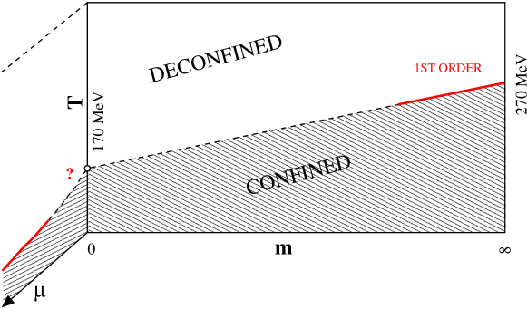
Figure 1: Schematic phase diagram of $N_{f}=2$ QCD.

Consider the plane $\mu=0$. As $m\to\infty$ quarks decouple and the system tends to the quenched limit. There the deconfining transition is well understood: the transition is an order-disorder first order phase transition, the symmetry involved is $Z_{3}$ and the Polyakov line $\langle L\rangle$ is an order parameter. In the presence of quarks $Z_{3}$ is explicitely broken and $\langle L\rangle$ is not a good order parameter. Empirically, however, it works as an order parameter at quarks masses down to $m\simeq 2.5-3$ GeV.

At $m\simeq 0$ a chiral phase transition takes place at $T_{c}\simeq 170$ MeV, from the low temperature phase where chiral symmetry is spontaneously broken to a phase in which it is restored: the chiral condensate $\langle\bar{\psi}\psi\rangle$ is the corresponding order parameter. At some temperature $T_{A}\geq T_{c}$ also the $U_{A}(1)$ symmetry, which is broken by the anomaly, is expected to be effectively restored.

It is not understood what the chiral transition has to do with the deconfining transition, but empirically the Polyakov line has a rapid increase at the transition temperature, indicating deconfinement.

More generally the transition line in Fig. 1 is defined by the maxima of a number of susceptibilities ($C_{V}$, $\chi_{m}$, $\dots$) which all coincide within errors, and which indicate a rapid variation of the corresponding parameters across the line.

A renormalization group analysis plus $\epsilon$-expansion techniques can be made at $m\simeq 0$, assuming that the relevant degrees of freedom for the chiral transition are scalar and pseudoscalar fields wilcz1 ; wilcz2 ; wilcz3 , or more precisely that the order parameters are the vacuum expectation values (v.e.v.) of the following fields

$$\tilde{\phi}:\ \ \phi_{ij}\equiv\langle\bar{q}_{i}(1+\gamma_{5})q_{j}\rangle\ \ \ \ (i,j=1,\ldots,N_{f})\,.$$ (1)

Under chiral and $U_{A}(1)$ transformations of the group $U_{A}(1)\otimes SU(N_{f})\otimes SU(N_{f})$, $\tilde{\phi}$ transforms as

$$\tilde{\phi}\rightarrow e^{i\alpha}U_{+}\tilde{\phi}U_{-}$$ (2)

so that by the usual symmetry arguments, and neglecting irrelevant terms

$${\cal L}_{\phi}=\frac{1}{2}Tr\{\partial_{\mu}\phi^{\dagger}\partial^{\mu}\phi\}-\frac{m_{\phi}^{2}}{2}Tr\{\phi^{\dagger}\phi\}-\frac{\pi^{2}}{3}g_{1}\left(Tr\{\phi^{\dagger}\phi\}\right)^{2}-\frac{\pi^{2}}{3}g_{2}Tr\{(\phi^{\dagger}\phi)^{2}\}+c\left[{\rm det}\phi+{\rm det}\phi^{\dagger}\right]\,.$$ (3)

The last term describes the anomaly: indeed it is $SU(N_{f})\otimes SU(N_{f})$ invariant, but not $U_{A}(1)$ invariant.

A second order phase transition corresponds to an infrared (IR) stable fixed point. For $N_{f}\geq 3$ the effective action is of the form Eq. (3) and no such point exists so that the transition is first order. For $N_{f}=2$, ${\rm det}\phi$ has mass dimension 2 so that other relevant terms emerge, like $({\rm det}\phi+{\rm det}\phi^{\dagger})^{2}$ and $Tr\{\phi^{\dagger}\phi\}({\rm det}\phi+{\rm det}\phi^{\dagger})$. If the anomaly term in Eq. (3) vanishes $(c\simeq 0)$, i.e. if the $\eta^{\prime}$ mass vanishes at $T_{c}$, then there is no IR stable fixed point and the transition is first order. If instead $c\neq 0$ the symmetry is $SU(2)\otimes SU(2)\simeq O(4)$ and a fixed point exists which can produce a second order phase transition.

In the first case the phase transition is first order also at $m\neq 0$ and most likely up to $m=\infty$.

In the second case a phase transition is only present at $m=0$, which goes into a continuous crossover as $m\neq 0$: this is true also in presence of a small chemical potential $\mu\neq 0$, so that a tricritical point is expected in the $T$-$\mu$ plane (see Fig. 1) at the border of the crossover with the first order transition line which takes place in the small $T$, large $\mu$ region Stephanov . Proposals exist to detect the tricritical point in heavy ion collisions: obviously no such point exists if the transition at $\mu=0$ is first order.

The issue is in fact fundamental. If confinement is an absolute property of the QCD vacuum and the deconfinement transition corresponds to a change of symmetry (order – disorder), then a crossover is excluded and the only allowed possibility is that the transition is always first order. The argument also extends to the case of $2+1$ flavors, of which Fig. 1 is a boundarycolombia . The question deserves a careful study.

A few groups have investigated the problem on the lattice with staggered fuku1 ; fuku2 ; colombia ; karsch1 ; karsch2 ; jlqcd ; milc or Wilson cp-pacs fermions. The strategy used has either been to look for signs of discontinuity at the transition, or to study the dependence on $m$ of the peak of different susceptibilities, or to study the magnetic equation of state. No clear sign of discontinuity has been observed, but also no conclusive agreement of scaling with $O(4)$ critical indexes. In particular the thermal exponent $y_{t}=1/\nu$ (see Sect. II for the definition) determined using staggered fermions differs significantly from that of $O(4)$-$O(2)$ (no direct determination of the critical exponents exists for Wilson quarks). A general tendency exists however in the community to consider the chiral transition second order, and the line of Fig. 1 a crossover.

In the present work we have made a big numerical effort and used large lattices attempting to clarify the issue. Like most of the other works we use non improved Kogut–Susskind action, and lattices $4\times L_{s}^{3}$ with $L_{s}=16,20,24,32$. Some scaling violations are expected and a more careful study with $L_{t}=6$ and an improved action is planned in order to control them.

A preliminary account has been presented at conferences D'Elia:2004ua . The present paper contains more data and a full analysis.

The paper is organized as follows: In Section II we explain the strategy used to attack the problem. Section III contains details about the simulations and the numerical results. Section IV contains the analysis of scaling. Section V contains a discussion and the conclusions.

II Strategy

The theoretical tool to investigate the order of a phase transition is finite size scaling FISHER72 ; BREZIN82 . The extrapolation from finite size $L_{s}$ to the thermodynamical limit $L_{s}=\infty$ is governed by the critical indexes, which identify the order and the universality class of the transition.

Approaching the transition, for a higher order or weak first order transition, the correlation length of the order parameter $\xi$ goes large compared to the lattice spacing $a$, so that the dependence of physical quantities on $a/\xi$ can be neglected. More precisely, if ${\cal L}/kT$ is the effective action (density of free energy)

$$\frac{\cal L}{kT}\simeq L_{s}^{-d}\phi\left(\frac{a}{\xi},\frac{L_{s}}{\xi},am_{q}L_{s}^{y_{h}}\right)$$ (4)

the dependence on $a/\xi$ disappears as $T_{c}$ is approached, since $\xi$ diverges as

$$\xi\simeq_{\tau\to\infty}\tau^{-\nu}$$ (5)

where $\tau\equiv 1-\frac{T}{T_{c}}$. The variable $L_{s}/\xi$ can be traded with $\tau L_{s}^{1/\nu}$ and the scaling law follows

$$\frac{\cal L}{kT}\simeq L_{s}^{-d}\phi\left(\tau L_{s}^{1/\nu},am_{q}L_{s}^{y_{h}}\right)\,.$$ (6)

The problem has two scales, $\xi$ and $1/m_{q}$. The effective action depends on the order parameter, as dictated by the symmetry, and as $\tau\to 0$ irrelevant terms can be neglected. The thermodynamics is described by correlators of the order parameter, which contain information on the discontinuities of the thermodynamical quantities. The most fundamental quantity is the specific heat, which is always guaranteed to exhibit the correct critical behaviour, independently of the identification of the correct order parameter.

For the specific heat the scaling law is

$$C_{V}-C_{0}\simeq L_{s}^{\alpha/\nu}\phi_{c}\left(\tau L_{s}^{1/\nu},am_{q}L_{s}^{y_{h}}\right)\,;$$ (7)

$C_{0}$ stems from an additive renormalization BREZIN82 .

For the susceptibility $\chi$ of the order parameter $O(x)$

$$\chi=\int d^{3}x\left[\langle O(x)O(0)\rangle-\langle O\rangle^{2}\right]$$ (8)

the scaling law is

$$\chi\simeq L_{s}^{\gamma/\nu}\phi_{\chi}\left(\tau L_{s}^{1/\nu},am_{q}L_{s}^{y_{h}}\right)\,.$$ (9)

We shall discuss the question if a subtraction is needed for $\chi$ as for the specific heat in Sect.IV.4.

Analogous scaling laws can be derived for mixed susceptibilities.

The values of the indexes characterize the transition: the values relevant to the analysis which follows are listed in Table 1. $O(4)$ is the symmetry expected if the chiral transition is second order, but it can break down to $O(2)$ by the lattice discretization for Kogut–Susskind fermions karsch1 at non zero lattice spacing.

	$y_{t}$	$y_{h}$	$\nu$	$\alpha$	$\gamma$	$\beta$	$\delta$
$O(4)$	1.336(25)	2.487(3)	0.748(14)	-0.24(6)	1.479(94)	0.3837(69)	4.852(24)
$O(2)$	1.496(20)	2.485(3)	0.668(9)	-0.005(7)	1.317(38)	0.3442(20)	4.826(12)
$MF$	$3/2$	$9/4$	$2/3$	0	1	1/2	3
$1^{st}Order$	3	3	$1/3$	1	1	0	$\infty$

Table 1: Critical exponents.

The scaling law in Eq. (7) for the specific heat is valid independent of the knowledge of the order parameter. The scaling law in Eq. (9) instead is correct only if the choice of the order parameter is the right one. In principle the matching between (7) and (9) can be used to legitimate any guess on the symmetry and on the order parameter.

The scaling laws (7) and (9) are difficult to test because they depend on two variables. A possible strategy is to keep one of them fixed and to study the scaling with respect to the other. As one can see in Table 1, the index $y_{h}$ is the same within errors for $O(4)$ and $O(2)$ symmetry. In order to reduce the problem to one scale, we have made a number of simulations at different values of $L_{s}$ and $am_{q}$ keeping $am_{q}L_{s}^{y_{h}}$ fixed and assuming $y_{h}=2.49$ which corresponds to $O(4)$ or $O(2)$. In this way as $L_{s}$ is increased, $am_{q}\to 0$, so that the infinite volume limit corresponds to the chiral transition at $am_{q}=0$.

From Eq.s (7) and (9) it follows that the maxima at constant $am_{q}L_{s}^{y_{h}}$ scale as

$$(C_{V}-C_{0})_{\rm max} \propto L_{s}^{\alpha/\nu}$$

$$\chi_{\rm max} \propto L_{s}^{\gamma/\nu}\,.$$ (10)

as $L_{s}\rightarrow\infty$ and their positions scale as

$$\tau L_{s}^{1/\nu}={\rm const}$$ (11)

If $O(4)$ or $O(2)$ is the correct symmetry, the values of $\alpha/\nu$ and $\gamma/\nu$ should be consistent with the corresponding values listed in Table 1.

Notice that Eq.s (7) and (9) involve the long range part of the correlations, i.e. they are related to the infrared regime, and are not expected to be significantly affected by scaling violations $O(a/\xi)$.

If the answer to this test is positive the chiral transition is second order at $am_{q}=0$ and a crossover at $am_{q}\neq 0$. If instead the answer is negative and the assumption of Ref.wilcz1 ; wilcz2 ; wilcz3 about the relevant degrees of freedom is correct, the transition is first order at $am_{q}=0$, and also at $am_{q}\neq 0$.

An alternative strategy can be as follows. At fixed $am_{q}$, $\beta$ the values of the susceptibility should converge at large $L_{s}$ if ${\cal L}$ is analytic. One can change variable by replacing $\tau L_{s}^{1/\nu}$ with the ratio

$$\frac{\tau L_{s}^{1/\nu}}{(am_{q}L_{s}^{y_{h}})^{1/(\nu y_{h})}}=\tau(am_{q})^{-1/(\nu y_{h})}\,.$$ (12)

The scaling laws Eq.s (7) and (9) become then

$$C_{V}-C_{0}\simeq L_{s}^{\alpha/\nu}\tilde{\phi}_{c}\left(\tau(am_{q})^{-1/(\nu y_{h})},am_{q}L_{s}^{y_{h}}\right)$$ (13)

$$\chi\simeq L_{s}^{\gamma/\nu}\tilde{\phi}_{\chi}\left(\tau(am_{q})^{-1/(\nu y_{h})},am_{q}L_{s}^{y_{h}}\right)\,.$$ (14)

At large $L_{s}$ the dependence on $am_{q}L_{s}^{y_{h}}$ must cancel the dependence on $L_{s}$ in front of the scaling functions in Eq.s (7) and (9). It follows that

$$C_{V}-C_{0}\simeq(am_{q})^{-\alpha/(\nu y_{h})}f_{c}\left(\tau(am_{q})^{-1/(\nu y_{h})}\right)$$ (15)

$$\chi\simeq(am_{q})^{-\gamma/(\nu y_{h})}f_{\chi}\left(\tau(am_{q})^{-1/(\nu y_{h})}\right)\,.$$ (16)

The peaks of $(C_{V}-C_{0})$ and of $\chi$ should then scale as

$$(C_{V}-C_{0})_{\rm max} \propto (am_{q})^{-\alpha/(\nu y_{h})}$$

$$\chi_{\rm max} \propto (am_{q})^{-\gamma/(\nu y_{h})}$$ (17)

as $am_{q}\rightarrow 0$. As for the position of the maxima, it scales according to

$$\tau(am_{q})^{-1/(\nu y_{h})}={\rm const}\,.$$ (18)

An alternative possibility is to keep the scaling in the form of Eq.s (7) and (9), and require that the volume dependence disappears at $\tau L_{s}^{1/\nu}$ fixed. This kind of scaling could work better if the correlation length is comparable to $L_{s}$, while $aL_{s}m_{\pi}\gg 1$. This implies the scaling laws:

$$C_{V}-C_{0}\simeq(am_{q})^{-\alpha/(\nu y_{h})}f_{c}\left(\tau L_{s}^{1/\nu}\right)$$ (19)

$$\chi\simeq(am_{q})^{-\gamma/(\nu y_{h})}f_{\chi}\left(\tau L_{s}^{1/\nu}\right)\,.$$ (20)

Eq.s (17) for the maxima stay unchanged, but the positions of the maxima scale now as

$$\tau L_{s}^{1/\nu}={\rm const}\,$$ (21)

and the width of the peaks are volume dependent.

All that is expected to be true at sufficiently large values of $aL_{s}\cdot m_{\pi}$ and at sufficiently small values of $am_{q}$, such that we are not too far from the critical point.

$\tau\equiv 1-T/T_{c}$ is usually taken in the literature karsch1 ; karsch2 as proportional to $\beta_{0}-\beta$, where $\beta_{0}$ is the value of $\beta=2N_{c}/g^{2}$ at the chiral $(am_{q}=0)$ transition, and all the analyses of the scaling law are based on that choice.

In fact, since

$$T=\frac{1}{L_{t}a(\beta,am_{q})}\,,$$ (22)

the correct definition is

$$\tau\equiv 1-\frac{T}{T_{c}}=1-\frac{a(\beta_{0},0)}{a(\beta,am_{q})}\,.$$ (23)

and the dependence on $am_{q}$ is non trivial (see e.g. massapi ). $a(\beta,am_{q})$ is expected to be an analytic function in a neighborhood of the critical point and therefore for sufficiently small $\beta_{c}-\beta$ and $m$

$$a(\beta,am_{q})\simeq a(\beta_{0},0)+\frac{\partial a}{\partial\beta}(\beta_{0},0)(\beta-\beta_{0})+\frac{\partial a}{\partial(am_{q})}(\beta_{0},0)am_{q}\,.$$ (24)

If needed higher orders in $am_{q}$ and $(\beta-\beta_{0})$ can be included. It then follows that at sufficiently small values of $am_{q}$

$$\tau=C(\beta_{0}-\beta+k_{m}am_{q})$$ (25)

with

$$C \equiv \frac{\partial\ln a}{\partial\beta}(\beta_{0},0)$$

$$k_{m} \equiv \frac{1}{C}\frac{\partial\ln a}{\partial am_{q}}(\beta_{0},0)\,.$$ (26)

In the quenched case this reduces to $\tau\propto\beta_{0}-\beta$ as usual: in the presence of dynamical quarks $k_{m}\neq 0$ massapi .

The scaling law for the position of the peaks becomes then

$$\beta_{0}-\beta_{c}+k_{m}am_{q}={\rm const}\cdot(am_{q})^{1/(\nu y_{h})}\,.$$ (27)

Eq.s (15) and (16) should be valid if $L_{s}\gg\xi/a$, $L_{s}\gg 1/(am_{\pi})$ (see Table 2). If the alternative possibility is considered, i.e. requesting that the free energy stays finite when $L_{s}\rightarrow\infty$ at fixed $\tau L_{s}^{1/\nu}$, the position scales instead as

$$\beta_{0}-\beta_{c}+k_{m}am_{q}={\rm const}\cdot L_{s}^{-1/\nu}\,.$$ (28)

Analogous formulae can be written including quadratic terms of the expansion Eq. (24) (see Section IV below).

An alternative technique is to investigate the order of the transition by looking for discontinuities: if the transition is first order at $m=0$, it is expected to be so also at $m\neq 0$. If the transition is weak first order, at small volumes compared to some critical volume it will behave as if the free energy were regular, so that Eq.s (15), (16) and (17), or (19) and (20), are expected to be valid, with the critical indexes appropriate to first order. At larger volumes, however, the peak of the specific heat as well as the peaks of the other susceptibilities should increase proportionally to the volume, as a consequence of the discontinuity in the first derivatives of the free energy. At the same time a bistability should appear in the time histories colombia . Such an analysis has been in particular performed in Ref.jlqcd ; milc : some sign of growth with the volume has been observed, but no significant bistability; we will comment on this result below. Of course if a discontinuity is observed one can conclude that the transition is first order. If not one cannot exclude that it could be observed at larger volumes.

Finally one can investigate the so-called magnetic equation of state milc , i.e. the scaling behaviour of the chiral order parameter itself, $\langle\bar{\psi}\psi\rangle$, versus the reduced temperature. The scaling law is

$$\langle\bar{\psi}\psi\rangle\simeq m^{1/\delta}f(\tau m^{-1/(\nu y_{h})})$$ (29)

and again it can provide information on the critical indexes.

III Numerical simulations

III.1 Algorithm

Monte Carlo simulations were performed using the standard staggered action. The Hybrid R algorithm HybridR was used for the configuration updating. Since it is a non-exact algorithm, its systematic errors must be kept under control. The finite integration step used in the molecular dynamics evolution introduces a systematic error on the mean values of observables proportional to the integration step squared $\Delta\tau^{2}$. Great care was taken to ensure that this systematic shift were much smaller than the statistical error in each Monte Carlo run. Typical values of the integration step $\Delta\tau$ vary with the mass of the quarks in units of the lattice spacing as $\Delta\tau=am_{q}/4$. When the use of that value for the integration step was too proibitive, i.e. at the smallest quarks masses used in this work, the integration step was in any case taken below $am_{q}/2$. The stopping condition used for the conjugate gradient inversion was fixed requiring that the residue were smaller than $10^{-8}$. The length of the molecular dynamics trajectories was fixed to $1$ for all of our simulations.

III.2 Run parameters

All of our numerical simulations were performed using a lattice temporal extent of $L_{t}=4$. To begin with we run two sets of Monte Carlo simulations fixing for each the value of $am_{q}L_{s}^{y_{h}}$ as explained in Section II. The two sets, called in the following Run1 and Run2, have $am_{q}L_{s}^{y_{h}}=74.7$ and $am_{q}L_{s}^{y_{h}}=149.4$ respectively. The spatial lattice sizes $L_{s}$ used for each of the two sets are $L_{s}=12,16,20,32$.

Additional simulations at $L_{s}=24$ and $am_{q}=0.04444$ and at $L_{s}=16$ and $am_{q}=0.01335$ were added. The second one was chosen by purpose at the same mass of the $L_{s}=32$ of Run1.

A summary of the bare quark masses and $L_{s}$ used is reported in Table 2. The total number of MC trajectories collected is also reported together with the quantity $aL_{s}\cdot m_{\pi}$ at the pseudocritical value of the coupling $\beta_{c}$ ($am_{\pi}$ was taken from the parametrization given by the MILC collaboration in Ref.massapi ). Since for all our runs the spatial extent is much larger than the pion correlation length, no large infrared cut-off effects are expected, except possibly for the run at $L_{s}=16$ and $am_{q}=0.01335$ (see Table 2).

Table 2: Run parameters for the numerical simulations.

	Run1				Run2				Other
$L_{s}$	12	16	20	32	12	16	20	32	16	24
$am_{q}$	0.153518	0.075	0.04303	0.01335	0.307036	0.15	0.08606	0.0267	0.01335	0.04444
# Traj.	22500	87700	14520	14500	25000	131390	16100	15100	10000	10000
$aL_{s}\cdot m_{\pi}$	11.9	11.0	10.0	8.9	11.3	15.8	14.8	12.4	4.5	12.2

For each value of $am_{q}$ and $L_{s}$ and for each run, MC simulations were performed at different $\beta$ values in order to inspect and to have under control the whole interesting critical region. See Appendix A for the whole listing of our run parameters.

III.3 Data Reweighting

The collected raw data were analyzed using standard statistical procedures (see e.g. newmanbarkema ). For the history of each observable, thermalizations were taken self consistently to be five times the integrated autocorrelation time estimated from thermalized trajectories.

The data collected were analyzed using the multi-histogram reweighting technique combining data taken at different $\beta$’s together. This method allows to extract mean values of observables and their susceptibilities at intermediate $\beta$ values over the whole range explored with numerical simulations. Using the reweighted data, it is possible to locate accurately the position at which the susceptibilities attain their maximum and their value at the maximum. Sometimes in previous studies a single point with high statistics at about the critical point was used. Using data from simulations done at several $\beta$ values covering the whole critical region, eliminates the risk of a wrong extrapolation from a single $\beta$ too distant from the critical point. Moreover the method allows a better sampling of the probability distribution, due to the fact that different simulations are combined together, thus increasing the precision and confidence of the measurement.

The errors of observable quantities were estimated using the bootstrap method. In practice, this means repeating the whole multi-histogram reweighting procedure a number of times starting from random data samples distributed as the measured empirical distributions.

III.4 Observables

For each generated configuration of our MC simulations we measured the average spatial and temporal plaquettes ($P_{\sigma}$, $P_{\tau}$), the chiral condensate ($\bar{\psi}\psi$), the energy density ($\bar{\psi}D_{0}\psi$) and the following lattice susceptibilities (the notation is the same as in jlqcd ):

$$\chi_{m}^{disc} = \left(\frac{N_{f}}{4}\right)^{2}\frac{1}{V}\left[\langle({\rm Tr}D^{-1})^{2}\rangle-\langle{\rm Tr}D^{-1}\rangle^{2}\right]$$ (30)

$$\chi_{m}^{conn} = -\frac{N_{f}}{4V}\sum_{x,y}\left<D_{x,y}^{-1}D_{y,x}^{-1}\right>$$ (31)

$$\chi_{e,ij} = V[\left<P_{i}P_{j}\right>-\left<P_{i}\right>\left<P_{j}\right>],\quad i,j=\sigma,\tau$$ (32)

$$\chi_{e,f} = V[\left<(\bar{\psi}D_{0}\psi)^{2}\right>-\left<\bar{\psi}D_{0}\psi\right>^{2}]$$ (33)

$$\chi_{e,i} = V[\left<P_{i}(\bar{\psi}D_{0}\psi)\right>-\left<P_{i}\right>\left<\bar{\psi}D_{0}\psi\right>],\quad i=\sigma,\tau$$ (34)

$$\chi_{t,i} = V[\left<P_{i}(\bar{\psi}\psi)\right>-\left<P_{i}\right>\left<\bar{\psi}\psi\right>],\quad i=\sigma,\tau$$ (35)

$$\ \chi_{t,f} = V[\left<(\bar{\psi}\psi)(\bar{\psi}D_{0}\psi)\right>-\left<(\bar{\psi}\psi)\right>\left<\bar{\psi}D_{0}\psi\right>]$$ (36)

where $V=L_{s}^{3}L_{t}$ is the volume; $D_{0}$ is the temporal component of the Dirac operator $D$.

The connected component of the chiral susceptibility $\chi_{m}^{conn}$ has not been measured for all of our simulations but only for a fraction of them. The method used to extract $\chi_{m}^{conn}$ is the volume source method without gauge fixing as described in Ref.jlqcd . The disconnected component gives the dominant contribution for large volumes and small masses. The connected part is instead relevant at small volumes and relatively large masses. For most of our lattices we have determined the connected part only around the peak, and we have considered it as a constant with respect to $\beta$. We estimate that this is a good approximation within our errors. A representative example is shown in Fig. 2 (taken at $L_{s}=24$, $am_{q}=0.04444$). The typical contribution to $\chi_{m}$ of $\chi_{m}^{conn}$ is less than about $15\%$ of $\chi_{m}^{disc}$ at the peak value and is a slowly varying function of $\beta$.

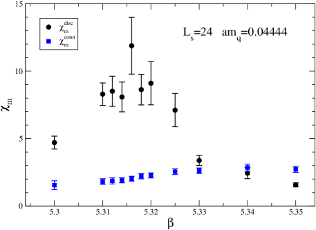
Figure 2: Comparison between the connected and disconnectd component of $\chi_{m}$. The former is typically a small fraction of the connected component at the peak position.

A comprehensive list of measured values of $\langle P_{\sigma}\rangle$, $\langle P_{\tau}\rangle$, $\langle\bar{\psi}\psi\rangle$, $\langle\bar{\psi}D_{0}\psi\rangle$ and the lattice susceptibilities for our MC simulation can be found in Appendix A.

IV Scaling analysis

The basic thermodynamic susceptibilities, i.e. the specific heat $C_{V}$, the chiral susceptibility $\chi_{m}$ and the mixed susceptibility $\chi_{t}$

$$C_{V} = \frac{1}{VT^{2}}\frac{\partial^{2}}{\partial(1/T)^{2}}\ln Z$$ (37)

$$\chi_{m} = \frac{T}{V}\frac{\partial^{2}}{\partial m_{q}^{2}}\ln Z$$ (38)

$$\chi_{t} = \frac{T}{V}\frac{\partial^{2}}{\partial(1/T)\partial m_{q}}\ln Z$$ (39)

can be expressed as sums of the lattice susceptibilities (30)-(36) multiplied by regular functions of $\beta$ and $am_{q}$. Specifically the specific heat $C_{V}$ is a function of $\chi_{e,ij}$, $\chi_{e,i}$ and $\chi_{e,f}$; $\chi_{t}$ is a function of $\chi_{t,i}$ and $\chi_{t,f}$. The contribution of other susceptibilities entering in the expression of $C_{V}$ and $\chi_{t}$ involving the quark mass are expected to be negligible in the chiral limit Karsch:1986ec . As for $\chi_{m}$, $\partial/\partial(m_{q})$ in Eq.(38) is intended at constant temperature. Since temperature depends not only on $\beta$ but also on $am_{q}$, the physical $\chi_{m}$ is a combination of $\chi_{m}^{disc}$, $\chi_{m}^{conn}$, $\chi_{t,\tau}$ and $\chi_{e,\tau\tau}$ with computable coefficients.

By $C_{V}$ in the following we mean $\chi_{e,\sigma\sigma}$; the analysis with $\chi_{e,i}$ and $\chi_{e,f}$ is similar and compatible with respect to scaling.

We are interested in studying the singular behavior of $C_{V}$, $\chi_{m}$ and $\chi_{t}$ as the critical surface is approached which is given by the most singular divergent quantity among the lattice susceptibilities corresponding to a given termodynamical susceptibility.

IV.1 Pseudocritical coupling

One of the observables analyzed in the literature to understand the order of the transition has been the position of the peaks of thermodynamic susceptibilities as a function of $am_{q}$. The position of all these peaks happen to coincide at given $am_{q}$ and $L_{s}$, thus defining a unique (pseudo)critical coupling $\beta_{c}(am_{q})$. Previous works in the literature assume $\tau\propto\beta_{0}-\beta$, a choice usually based on a strict analogy between QCD and the $O(4)$ statistical model. In fact the correct thermodynamical reduced temperature is given by Eq. (23). In principle the dependence of $a(\beta,am_{q})$ on $am_{q}$ could be measured by use of independent quantities (see e.g. massapi ). We will try a fit of the position of $\beta_{c}$ by a form like Eq. (27) or (28), which is expected to be valid at sufficiently small values of $am_{q}$. To extend the range of validity of the approximation the quadratic terms proportional to $am_{q}^{2}$, $am_{q}(\beta_{0}-\beta)$ and $(\beta_{0}-\beta)^{2}$ may be added:

$$\tau\propto(\beta_{0}-\beta)+k_{m}am_{q}+k_{m^{2}}(am_{q})^{2}+k_{m\beta}am_{q}(\beta_{0}-\beta)\,.$$ (40)

A term $k_{\beta^{2}}(\beta_{0}-\beta)^{2}$ turns out to be negligible. In fact one can write the lattice spacing $a$ as:

$$a=\frac{1}{\Lambda(\beta,am_{q})}\left(\frac{\beta}{4N_{c}b_{0}}\right)^{\frac{b_{1}}{2b_{0}^{2}}}\exp\left(-\frac{\beta}{4N_{c}b_{0}}\right)$$ (41)

where the deviation from asymptotic scaling are represented by the fact that the term $\Lambda(\beta,am_{q})$ is $\beta$ dependent. This term is slowly varying with $\beta$ and can be well described by a linear function of $\beta$ with coefficients depending on $am_{q}$ in the relevant range of $\beta$’s. The $k_{\beta^{2}}$ coefficient is given by $\partial^{2}\ln a/\partial\beta^{2}|_{\beta=\beta_{0},am_{q}=0}$ can be computed and can be neglected within errors. The other unknown parameters can be fitted to the data.

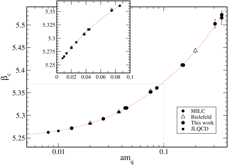
Figure 3: (Pseudo)critical couplings determined in this work are shown together with other determinations form the literature. Logarithmic scale is used for the horizontal scale in the main figure, while a linear scale is used for the smaller inset figure. The dotted line is the best fit ($\chi^{2}/d.o.f=0.89$, $d.o.f.=15$) curve including $am_{q}^{2}$ and $am_{q}(\beta_{0}-\beta_{c})$ terms for masses $am_{q}<0.4$.

Fig. 3 shows the critical line $\beta_{c}(am_{q})$. Our determinations are reported together with a collection of world data. A good agreement among different determinations can be appreciated.

The expected variation of $\tau$ as a function of $am_{q}$ or $L_{s}$ is given by Eq. (18) or (21):

$$\tau = k_{\tau}(am_{q})^{1/\nu y_{h}}\,\,\,\,\,\,\,\rm{or}$$ (42)

$$\tau = k^{\prime}_{\tau}L_{s}^{1/\nu}\,\,\,.$$ (43)

Notice that for a first order transition the exponent of $am_{q}$ is $1$ and the term on the right hand side of Eq. (42) can be reassorbed in $k_{m}$ so that such term can be discriminated only for a second order scaling behavior.

The unknown coefficients $k_{m}$, $k_{m^{2}}$, $k_{m\beta}$ and $k_{\tau}$ of the expansion of $\tau$ around the critical point are determined by use of a best fit procedure. We start from the form Eq. (43). In agreement with previous works we find that the position of the peaks does not depend on the lattice size karsch1 ; jlqcd , i.e. that $k^{\prime}_{\tau}=0$ within errors implying that no information can be obtained about the order of the transition (first order or second order $O(4)$ or $O(2)$). The quality of the fit assuming $k^{\prime}_{\tau}=0$ is shown in Fig. 3 and the resulting coefficients are listed in the first line of Table 3. These coefficients are obtained by a best fit up to a maximum value of $am_{q}$, $(am_{q})_{max}$, which is then extrapolated to zero. They are stable and consistent with a linear fit at low values of $am_{q}$ ($<0.0267$) as shown in the second line of Table 3.

The scaling of Eq. (21) or (43) assumes that $aL_{s}m_{\pi}\gg 1$ but the correlation length $\xi$ can be comparable with $L_{s}$, which is certainly true sufficiently close to the critical point in case of a second order or weak first order chiral transition.

We have then analyzed the scaling of the form Eq. (18) or (42). If the transition is first order the analysis coincides with the analysis done for the scaling Eq. (43) and $k_{m}$ is in fact $k_{m}-k_{\tau}$.

If the transition is $O(4)$ a similar analysis can be performed (similar results hold for $O(2)$ or mean field). The $\chi^{2}/d.o.f$ is acceptable, the result for the coefficients is shown in the third line of Table 3. $k_{\tau}$ is consistent with zero, and the result is therefore compatible with that of the first line. However the fit becomes unstable if we try to extrapolate to low masses keeping only the linear term of Eq.(40) (line 4 of Table 3).

The critical coupling $\beta_{0}$ and the coefficient $k_{m}$ are stable both for first order and $O(4)$ behavior and can thus be confidently estimated. Our final estimates, obtained by a weighted average of linear and quadratic fits, are $\beta_{0}=5.2484(5)$ and $k_{m}=1.82(8)$ for a first order transition; $\beta_{0}=5.2435(25)$ and $k_{m}=1.13(19)$ for $O(4)$. Other terms cannot be reliably estimated with present data. In particular we are not able to discriminate the contribution of quadratic terms from that coming from $k_{\tau}$ and consequently it is not possible to establish the order of the transition by looking at the (pseudo)critical couplings alone.

Table 3: Best fit parameters for the scaling of the pseudocritical coupling. Different kind of fits are explained in the text. $k^{\prime}_{\tau}$ is set to zero as explained in the text.

$\beta_{0}$	$k_{m}$	$k_{\tau}$	$k_{m^{2}}$	$k_{m\beta}$
5.2484(4)	1.84(7)	$\equiv 0$	-0.3(2.4)	-4.3(2.7)
5.2481(13)	1.75(13)	$\equiv 0$	$\equiv 0$	$\equiv 0$
5.2430(40)	1.20(60)	-0.1(1)	-7(6)	6(6)
5.2437(21)	1.12(16)	-0.134(46)	$\equiv 0$	$\equiv 0$

The possibility to discriminate between the first order and $O(4)$ behavior from the measurement of $\beta_{c}$ is in practice very faint. Fig. (4) shows the different predictions for the (pseudo)critical coupling based on available data. If we discard the high values of the masses a possible difference would only be visible at very small bare quark masses. Using estimates of $k_{\tau}$ shown in Table 3 a quark mass of about $0.003$ should be used, which requires a big numerical effort.

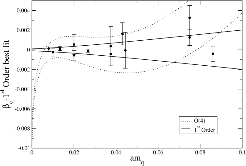
Figure 4: Different behavior of predicted (pseudo)critical couplings for a first order transition and a second order $O(4)$. Present data do not permit a clear discrimination using only $\beta_{c}$. The 1$\sigma$ band is displayed. Continuous lines correspond to a first order transition while the dotted lines are the prediction for the $O(4)$ symmetry.

We would like to remark that the explicit dependence of $\tau$ on $am_{q}$ is in any case necessary to fit present data. Fitting to a function of the form

$$\beta_{c}=\beta_{0}+c_{\tau}(am_{q})^{y_{t}/y_{h}}$$ (44)

with $O(4)$ values for the exponents, gives a $\chi^{2}/d.o.f\simeq 21$ in the interval up to $(am_{q})_{max}=0.075$, which decreases as $(am_{q})_{max}$ decreases and is $\approx 2$ at $(am_{q})_{max}=0.02$.

As a final remark, the dependence on $\beta$ and $am_{q}$ of the lattice spacing $a$ Eq. 23 can be measured from other observables (see e.g. massapi ). In particular our estimate for $k_{m}$ for a first order transition (line 1 of Table 3) is compatible with those of Ref. massapi $k_{m}\approx 1.95$ (affected by errors of order 20%). We notice that $k_{\tau}=0$ implies that $\tau=0$ on the critical line, or, by Eq. (24) that the critical temperature is independent of $am_{q}$ near the chiral point.

IV.2 Scaling at fixed $am_{q}L_{s}^{y_{h}}$

As explained in details in Section II, we have adopted a novel strategy in order to simplify the two scales problem. We assume $O(4)$ — or $O(2)$ — critical behaviour and we use this assumption to fix a dependence between $am_{q}$ and $L_{s}$ in our Run1 and Run2 so as to fix the second scaling variable in Eq. (6) and reduce the problem to a one scale problem: in this case the only assumption is $O(4)$ itself. This allows us to test whether $O(4)$ is consistent or not with data without any further approximation.

We fixed $am_{q}L_{s}^{y_{h}}=const$ with $y_{h}=2.49$ that is the value expected for $O(4)$ and $O(2)$ critical behavior, with $const=74.7$ for our Run1 and $const=149.4$ for Run2. The following scaling formulas should hold (see Eq.s (7) and (9)):

$$C_{V}(\tau,L_{s})-C_{0}=L_{s}^{\alpha/\nu}\Phi_{C}(\tau L_{s}^{1/\nu})$$ (45)

$$\chi_{m}(\tau,L_{s})=L_{s}^{\gamma/\nu}\Phi_{\chi}(\tau L_{s}^{1/\nu})$$ (46)

and in particular the peaks of the specific heat and $\chi_{m}$ should scale as Eq.s (10).

The subtraction of the non critical part $C_{0}$ for the specific heat is needed. In principle it can be obtained as a parameter from the fit to the maxima of the specific heat. However since we also have data at $\beta$’s different from the pseudocritical coupling, we were able to perform a direct measurement of this quantity. Appendix B reports the details of the study of the background for $C_{V}$. Our final estimate for the background is $C_{0}(\beta)=0.400(43)-0.0663(83)\beta$. Note that the $\beta$ dependence is very weak and assuming a constant value for the background $C_{0}$ does not modify the following analysis. No dependence of $C_{0}$ on $am_{q}$ is observed.

For the susceptibility of the chiral condensate $\chi_{m}$, for the moment we do not operate any bakground subtraction.

The measured peak values for the subtracted specific heat $C_{V}-C_{0}$ and chiral condensate susceptibility $\chi_{m}$ for Run1 and Run2 are shown in Fig. 5. They are evaluated on the curve obtained by reweighting.

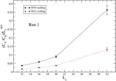
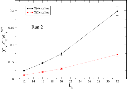
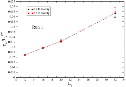
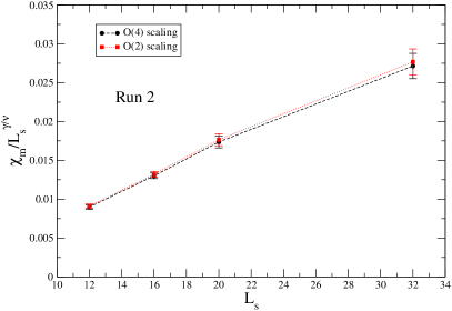
Figure 5: Specific heat (top) and $\chi_{m}$ (bottom) peak value for Run1 (left) and for Run2 (right), divided by the appropriate powers of $L_{s}$ (Eq.s 45-46) to give a constant. Both the $O(4)$ and $O(2)$ critical behaviors are displayed. Notice that for the case of $\chi_{m}$ the ratio $\gamma/\nu$ have almost the same numerical value so that the two curves are almost indistinguishable.

The figure shows the peak values of susceptibilities rescaled by the appropriate power of the spatial lattice size Eq. (10). If the scaling laws (10) would hold, the displayed quantity should be a constant. Visibly this is not the case.

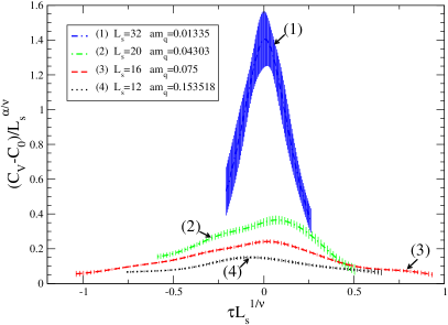
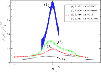
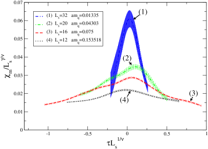
Figure 6: Scaling of the specific heat (top) and $\chi_{m}$ (bottom) for Run1 (left) and for Run2 (right), see Eq.s (7) and (9). The curves are obtained by reweighting.

The $O(4)$ and $O(2)$ critical behavior is clearly in contradiction with the lattice observation. In particular $O(4)$ and $O(2)$ scaling predicts no singular behavior in the $L_{s}\rightarrow\infty$ limit for the specific heat as the critical exponent $\alpha$ is negative. This means that as $L_{s}$ is increased, the singular part of $C_{V}$ should decrease with volume, i.e. that the specific heat should not grow which is in clear contrast with the data. Also for the chiral condensate susceptibility $\chi_{m}$ the predicted exponents fail to reproduce lattice data. In either case the $\chi^{2}/d.o.f.$ of the fit with a constant function excludes the behavior of scaling law (10). The full scaling laws Eq.s (7) and (9) were also studied (see Fig.(6)). The horizontal scale was obtained by fitting the pseudocritical temperature as described above. As one can expect from the previous discussion, data don’t scale according to the predicted laws.

Similar figures are obtained assuming $O(2)$ symmetry.

IV.3 Scaling at $L_{s}\rightarrow\infty$

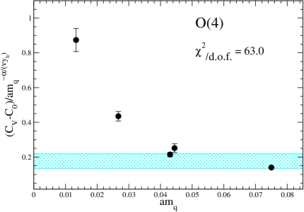
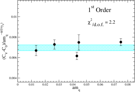
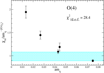
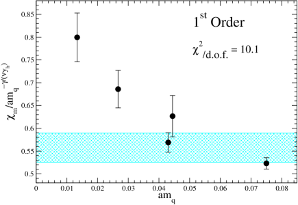
Figure 7: Specific heat (top) and $\chi_{m}$ (bottom) peak scaling for $O(4)$ (left) and first order (right).

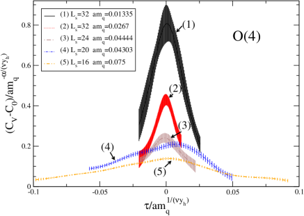
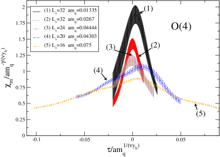
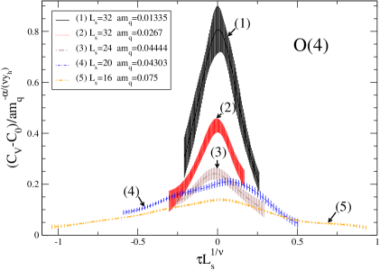
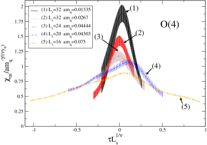
Figure 8: Comparison of specific heat (left) and $\chi_{m}$ (right) scaling for $O(4)$. Eq.19, 20 (top) and Eq.7, 9 (bottom).

A further scaling test can be done supposing that the lattice size is much larger that all other relevant physical lengths. In such a case one expects that the system show the same behavior of an infinite system. The scaling laws expected in this case are those of Eq.s (15) and (16). These equations predict no dependence on the parameter $L_{s}$. This is the same assumption used in previous scaling analyses of the chiral transition karsch2 ; jlqcd ; milc .

The alternative possibility, illustrated in section II, is to keep $\tau L_{s}^{1/\nu}$ (i.e. $\xi/(aL_{s})$) fixed thus remaining with the scaling equations Eq.s (19) and (20). Physically this means that the correlation length $\xi$ is not small compared to $L_{s}$, which is certainly true in the vicinity of the critical point.

These scaling laws are only expected to hold for large values of $am_{q}L_{s}^{y_{h}}$ and small masses.

The difference between the two alternatives is only visible by considering the width of the susceptibilities peaks, the heights having the same behavior (see Eq.s(17)).

We have thus first performed the analysis of the scaling of the maxima of the specific heat $C_{V}$ and $\chi_{m}$.

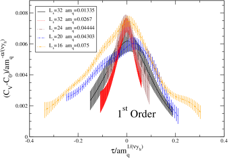
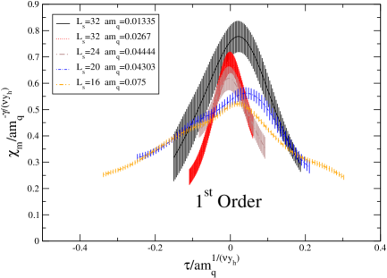
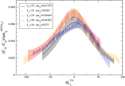
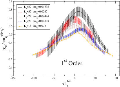
Figure 9: Comparison of specific heat (top) and $\chi_{m}$ (bottom) scaling for first order. Eq.19 and 20.

We have tested the different second order critical behaviors compatible with the scenario of Ref. wilcz1 , namely $O(4)$, $O(2)$, Mean Field and first order. The peak value of the specific heat and of $\chi_{m}$ divided by the appropriate power of the quark mass should be a constant. These ratios are shown in Fig.(7) both for $O(4)$ and first order. The figure shows also the confidence region from a fit with a constant value together with the corresponding $\chi^{2}$/d.o.f.

From the values of the $\chi^{2}$/d.o.f. it is easily seen that the second order critical behavior is not compatible with data. It must be noticed that, although the validity region of the scaling law is not known a priori, so that the upper mass limit for the fits is somewhat arbitrary, if we further restrict the mass region, the $\chi^{2}/d.o.f.$ for the $C_{V}$ fits tend to increase. We stress that also in previous studies karsch2 ; jlqcd ; milc the values found for the susceptibility peaks were not compatible with the critical indexes of $O(4)$, $O(2)$ and Mean Field. On the contrary the first order behavior looks compatible with data (even if the $\chi^{2}/d.o.f.$ is $\sim 2$) for the specific heat. We will discuss the scaling of $\chi_{m}$ in Sect.IV.4.

The scaling of susceptibilities at all $\beta$ values can also be investigated. The situation is depicted in Fig. 8 for $O(4)$: all the curves should coincide within errors if there were $O(4)$ scaling. Similar features are observed for $O(2)$ and Mean Field. No scaling is observed: this is clearly the case for the maxima of the susceptibilities as discussed above, but it is also true for the width of these curves. The analogous figure using first order indexes is shown in Fig. 9. Scaling is observed for the specific heat in the form Eq.s (19) and (20) and not in the form (15) and (16), which does not describe the widths of the peaks. Again for $\chi_{m}$ we postpone the discussion to Sect.IV.4.

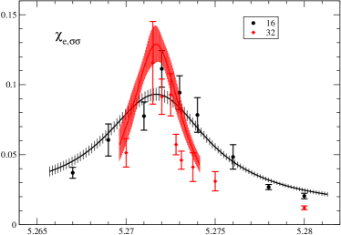
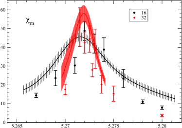
Figure 10: Comparison between $\chi_{e,\sigma\sigma}$ (left) and $\chi_{m}$ (right) for $am_{q}=0.01335$ and $L_{s}=16,32$.

Runs with higher values of the masses ($am_{q}>0.075$) do not obey the scaling laws. The one with $L_{s}=16$ and $am_{q}=0.01335$, which should coincide with the $L_{s}=32$ at the same bare mass, in case of scaling Eq.s (15) and (16) is instead different (see Fig. 10). For scaling Eq.s (19) and (20), the maximum should be the same, and the widths should differ by a factor of 8, and this is not the case. We have carefully checked the stability of the curves obtained by reweighting against variations of the statistics, e.g. by discarding single data points from the analysis. This lack of scaling can be interpreted as due to the small value (4.5) of the parameter $aL_{s}m_{\pi}$, invalidating the limit bringing to Eq.s (15), (16), (19) and (20). A similar effect could be responsible for the observed increase of the peak with the volume observed in previous studies jlqcd .

A more careful study of this effect will be done in the future.

IV.4 Magnetic equation of state

As a further test of scaling we check the equation of state Eq. (29). No scaling whatsoever is observed, neither $O(4)$-$O(2)$ nor first order, if the raw measured data are introduced in Eq.(29) (see Fig.11).

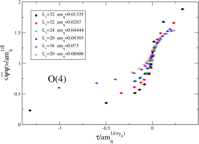
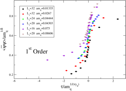
Figure 11: Magnetic equation of state using non subtracted data for $O(4)$ (left) and first order (right).

Indeed as $\langle\bar{\psi}\psi\rangle$ is different from 0 at large $\beta$ a subtraction is needed: the critical part of the chiral condensate has to be zero far above the critical region. A tentative way to understand the non critical background can be to assume it equal to the value $\langle\bar{\psi}\psi\rangle_{\infty}$ of $\langle\bar{\psi}\psi\rangle$ at $\beta=\infty$. This can be computed analytically and numerically on the flat configuration $U_{\mu\nu}=1$. The result is

$$\langle\bar{\psi}\psi\rangle_{\infty}(am_{q})=\frac{3}{L_{s}^{3}L_{t}}\sum_{k_{1},k_{2},k_{3},k_{4}}\frac{am_{q}}{(am_{q})^{2}+\sum_{i=1,2,3}(\sin\frac{\pi}{L_{s}k_{i}})^{2}+(\sin\frac{\pi}{L_{t}(k_{4}+1/2)})^{2}}$$ (47)

which is almost a linear function in the mass range $am_{q}<0.1$.

We then plot the subtracted value $\langle\bar{\psi}\psi\rangle_{s}\equiv\langle\bar{\psi}\psi\rangle-\langle\bar{\psi}\psi\rangle_{\infty}$ rescaled as $\langle\bar{\psi}\psi\rangle_{s}/(am_{q})^{1/\delta}$ versus $\tau(am_{q})^{-1/(\nu y_{h})}$ to test the scaling Eq. (29). Fig. 12 shows the result for $O(4)$ (similar figures being obtained with $O(2)$ and mean field). Visibly $O(4)$ scaling is not obeyed. An analogous investigation has been performed in Ref. milc , without the subtraction of the $\beta=\infty$ term: also in that case results were in disagreement with $O(4)$ scaling.

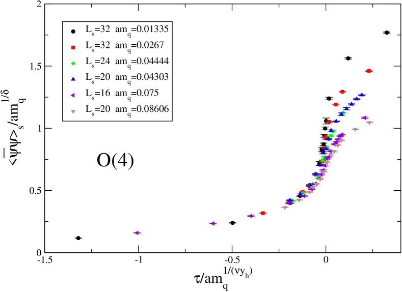
Figure 12: Equation of state for $O(4)$, obtained by subtraction of $\langle\bar{\psi}\psi\rangle$ at $\beta=\infty$.

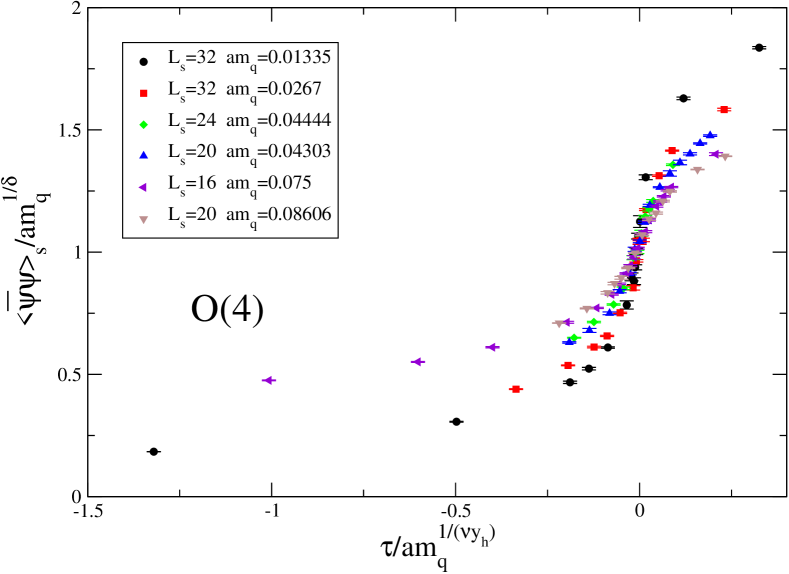
Figure 13: Equation of state for $O(4)$, obtained by imposing scaling at $\tau=0$.

An alternative procedure is to subtract for each $(am_{q},L_{s})$ the value at the largest measured $\beta$. The result is consistent with Fig. 12. A third possibility is to impose scaling at $\tau=0$ and look if it is obeyed at $\tau\neq 0$. The result is shown in Fig. 13 and again there is no scaling.

If the analysis of wilcz1 is correct, our results, which exclude a second order critical behavior, should then imply a first order chiral transition.

As a test of this possibility we have repeated the scaling analysis of the equation of state using first order critical indexes: the three procedures described above are consistent with each other and the result is shown in Fig. 14.

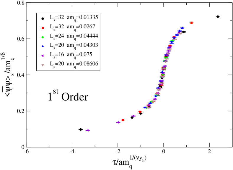
Figure 14: Equation of state for first order.

A good scaling is observed.

We can investigate the consequence of the subtraction needed to isolate the critical part of $\langle\bar{\psi}\psi\rangle$ on the scaling of $\chi_{m}$. If $\langle\bar{\psi}\psi\rangle-\langle\bar{\psi}\psi\rangle_{\infty}=am_{q}^{1/\delta}F(\tau/am_{q}^{1/\nu y_{h}})$ by differentiating with respect to $am_{q}$ at fixed temperature we get

$$\chi_{m}-\frac{\partial}{\partial am_{q}}\langle\bar{\psi}\psi\rangle_{\infty}=\frac{1}{\delta}am_{q}^{1/\delta-1}F-\frac{1}{\nu y_{h}}am_{q}^{1/\delta-1}(\tau/am_{q}^{1/\nu y_{h}})F^{\prime}$$ (48)

Keeping in mind $1/\delta=(d-y_{h})/y_{h}$, $\gamma=(2y_{h}-d)/y_{t}$ and $\nu=1/y_{t}$ we find, at $\tau=0$

$$am_{q}^{\gamma/\nu y_{h}}\left(\chi_{m}-\frac{\partial}{\partial am_{q}}\langle\bar{\psi}\psi\rangle_{\infty}\right)=\frac{1}{\delta}F(0)$$ (49)

The quantity which scales is not $am_{q}^{\gamma/\nu y_{h}}\chi_{m}$ but a term $am_{q}^{\gamma/\nu y_{h}}\partial\langle\bar{\psi}\psi\rangle_{\infty}/\partial(am_{q})$ must be added to it to get scaling. The subtraction of $\langle\bar{\psi}\psi\rangle$, due to the explicit breaking of chiral symmetry at $am_{q}\neq 0$, implies a subtraction for $\chi_{m}$ (which in the mass range of interest is almost constant).

This suggests to repeat the test of scaling for $\chi_{m}$ (Fig.s 5,6,7 and 8) by introducing a subtraction by a constant to be determined. The content of Fig. 10 instead stays unchanged since the curves refer to the same value of the mass.

The best fit to determine the background is done by requesting scaling for the peaks of $\chi_{m}$. the result is shown in Fig.s 5^′ and 7^′. For $O(4)$ —and $O(2)$— no scaling is obtained. A reasonable scaling results for first order. The corresponding modified scaling at all $\beta$’s is shown in Fig.s 6^′ and 8^′.

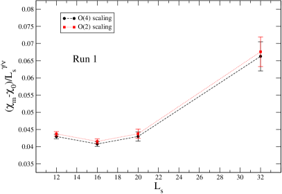
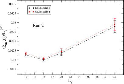
Figure 5^′: Scaling of the maxima of $\chi_{m}-\chi_{0}$ at fixed $am_{q}L_{s}^{y_{h}}$ for Run1 (left) and Run2 (right). Two curves are shown corresponding to $O(4)$ (circles) and $O(2)$ (squares) critical behavior. The value of $\chi_{0}$ is obtained by a best fit procedure.

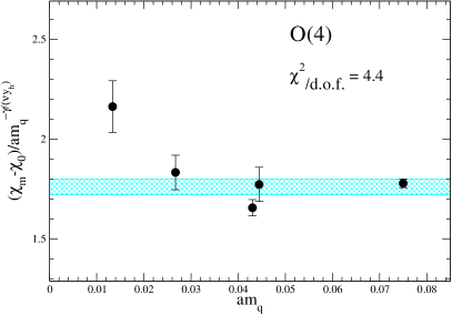
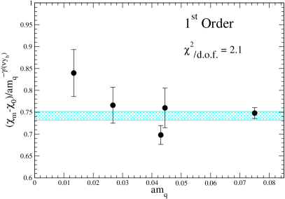
Figure 7^′: Scaling of the maxima of $\chi_{m}-\chi_{0}$ at small $am_{q}$ for $O(4)$ (left) and first order (right).The value of $\chi_{0}$ is obtained by a best fit procedure. The $\chi^{2}/d.o.f$ of the best fit is also shown.

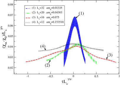
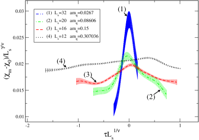
Figure 6^′: Scaling of subtracted chiral condensate $\chi_{m}-\chi_{0}$ for Run1 (left) and Run2 (right). The background value $\chi_{0}$ is obtained from a best fit of the peak value.

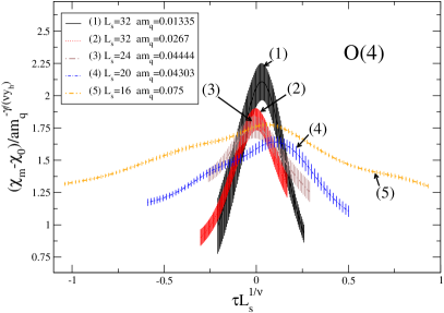
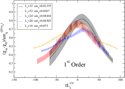
Figure 8^′: Scaling of subtracted chiral condensate $\chi_{m}-\chi_{0}$ at small $am_{q}$ for $O(4)$ (left) and first order (right). The background value $\chi_{0}$ is obtained from a best fit of the peak value.

We notice that, due to the dependence of the temperature $T$ on $am_{q}$ and not only on $\beta$ the definition of $\langle\bar{\psi}\psi\rangle=\frac{\partial\ln Z}{\partial m}|_{T}$ and $\chi_{m}=\frac{\partial^{2}\ln Z}{\partial m^{2}}|_{T}$ must be revised, resulting in a combination of several terms analogous to what happens for the specific heat.

Analogously to what has been done for the specific heat, we have not refined consequently our analysis. Our investigation is exploratory: our $L_{t}$ is not big enough, our action is not improved. We will extensively use the correct definitions in the planned improved version of this investigation.

IV.5 Metastabilities

A first order chiral transition implies first order also at $m\neq 0$ and this should be visible in time histories. Metastable states should be present and should be visible as double peak structures in the histograms of distributions of the value of observables for large enough volumes. Although the results for scaling presented in the previous sections indicate that our volumes are not large enough, we have analyzed the probability distribution function of a number of observables, in particular of the spatial plaquettes. The results are shown in Fig. 15. As in previous works fuku1 ; jlqcd no convincing metastability appears.

To estimate the probability distribution function (PDF) from a given finite data set a non-zero width of the integration region should be chosen. We assume for the width a value given by one hundredth of the difference between the largest and smallest entry in our dataset. Errors are estimated using the bootstrap technique.

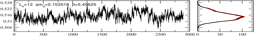
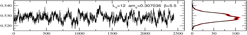
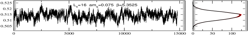
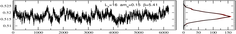
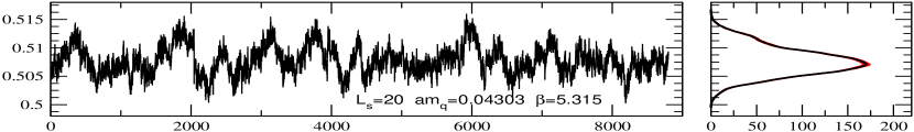
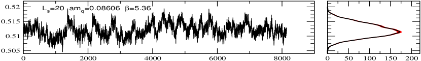
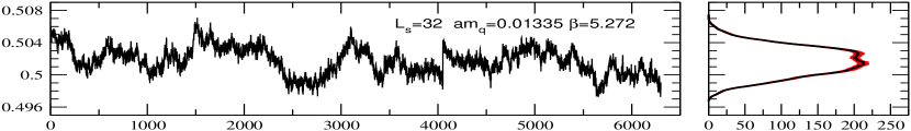
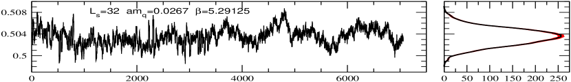
Figure 15: Probability distribution function of average plaquette. Chiral condensate shows a similar behavior.

V Discussion and conclusions

The study of the nature of the chiral transition of $N_{f}=2$ QCD is of fundamental importance: a second order phase transition would mean crossover at $m\neq 0$ and also at finite chemical potential, implying the presence of a tricritical point in the $T-\mu$ plane detectable by heavy ion experiments; a first order phase transition would drastically change this scenario. Moreover this is relevant to understanding what confined and deconfined really means in Nature, i.e. if they are two different phases of matter corresponding to different realizations of some symmetry with an order parameter, or are connected by a crossover.

Previous studies on the subject did not come to a definite conclusion, mainly because of the huge computer power required. We have approached the problem by dedicating a big amount of computer power and by proposing a novel strategy for the scaling study around the chiral critical point. In particular we have developed a scaling study which assumes the critical indexes of the expected second order universality class ($O(4)$ or $O(2)$ according to the analysis of Ref. wilcz1 ) to reduce to a one scale problem without any further assumption. In this way we have been able to definitively rule out the possibility of $O(4)$ or $O(2)$ critical indexes.

We have introduced the mass dependence of the reduced temperature $\tau$ (Eq. 23), which was neglected in previous works.

We have then analyzed our data to test the scaling as done in previous papers, assuming to be already in the thermodynamical limit (Eq. 15 and 16). The $am_{q}$ dependence of the pseudocritical $\beta$ can not discriminate between $O(4)$, $O(2)$ and first order. However the behavior of the peak of both the specific heat and of the chiral susceptibility definitely excludes $O(4)$ and $O(2)$, but are qualitatively consistent with first order (Fig. 7 and 7^′).

As for the shape of the critical peaks again $O(4)$ and $O(2)$ are definitely ruled out. The dependence of the width on $L_{s}$ shows that the thermodynamic limit is not reached. Instead a scaling at $L_{s}/\xi$ fixed agrees with first order, and again definitely excludes $O(4)$ and $O(2)$.

The magnetic equation of state is also nicely compatible with first order.

No clear signal of metastability, except possibly some hint, is observed.

In conclusion in $N_{f}=2$ QCD the chiral phase transition is not in the universality class of $O(4)$. Data strongly indicate a first order phase transition. Further study is needed to put this statement on a firmer basis. First we are planning a similar analysis with improved action and $L_{t}=6$. A consistency check will also be the study of the $\eta^{\prime}$ mass at the deconfining transition, in accordance with the analysis of wilcz1 , and we are also working at it.

Appendix A Monte Carlo parameters and raw data

In this appendix we report the details of our numerical results. Time histories of the observables are also available at request.

In the early stages of the computations some of the susceptibilities were not measured. Blank entries in the following tables refer to missing data.

In some previous report the data for the plaquette susceptibilities were defined with an extra factor of $1/4$. Below we have eliminated it in agreement with definition Eq. (32) to (36).

The connected component $\chi_{m}^{conn}$ has been measured only at the $\beta$ value nearest to the critical coupling (except for the run with $L_{s}=24$, $am_{q}=0.04444$).

Table 4: Mean value of plaquettes, chiral condensate and energy density from MC simulation. The number of thermalized trajectories is also shown together with the extimated autocorrelation time (for $P_{s}$ and $\langle\bar{\psi}\psi\rangle$)

$\beta$	# Traj.	$P_{\sigma}$	$P_{\tau}$	$\langle\bar{\psi}\psi\rangle$	$\langle\bar{\psi}D_{0}\psi\rangle$	$\tau_{int}$ ($P_{\sigma}$)	$\tau_{int}$ ($\langle\bar{\psi}\psi\rangle$)
$L_{t}$=4 $L_{s}$=12 $am_{q}$=0.153518
5.3	1300	0.47880(16)	0.47893(16)	1.07450(60)	—	7.7(2.4)	1.47(20)
5.325	1300	0.48578(17)	0.48601(17)	1.04638(59)	—	7.3(2.2)	1.71(26)
5.35	1300	0.49337(21)	0.49363(20)	1.01300(79)	—	10(3.7)	3.90(87)
5.375	2930	0.50082(12)	0.50130(13)	0.97909(55)	0.72133(24)	9.2(2.0)	3.71(53)
5.375	1250	0.50147(15)	0.50177(15)	0.97683(56)	—	6.0(1.7)	1.91(31)
5.3875	2860	0.50637(16)	0.50689(16)	0.95072(81)	0.72657(24)	12(3.2)	6.4(1.2)
5.3875	1200	0.50653(30)	0.50711(32)	0.9497(20)	—	18(9.3)	15(6.9)
5.4	2920	0.51129(16)	0.51196(18)	0.9233(11)	0.73140(25)	9.7(2.2)	8.3(1.8)
5.4	1200	0.51041(27)	0.51105(34)	0.9275(20)	—	13(5.9)	16(7.7)
5.40625	2890	0.51494(30)	0.51576(36)	0.8990(26)	0.73594(34)	32(14)	33(14)
5.40625	600	0.51464(37)	0.51582(34)	0.8986(31)	—	14(8.9)	16(10)
5.4125	2890	0.51762(50)	0.51869(57)	0.8796(43)	0.74062(55)	72(46)	77(51)
5.4125	1200	0.51955(36)	0.52100(49)	0.8635(37)	—	22(12)	36(25)
5.41875	2900	0.52200(36)	0.52357(40)	0.8470(28)	0.74866(41)	46(23)	42(20)
5.41875	840	0.52247(49)	0.52409(53)	0.8468(37)	—	20(13)	28(17)
5.425	2970	0.52508(18)	0.52692(23)	0.8255(17)	0.75432(29)	13(3.5)	19(6.3)
5.425	1200	0.52576(35)	0.52774(37)	0.8204(29)	—	19(9.8)	20(11)
5.43125	2910	0.52802(19)	0.52990(21)	0.8063(15)	0.75839(24)	17(5.4)	16(5.2)
5.43125	540	0.52952(58)	0.53151(70)	0.7917(61)	—	40(44)	66(90)
5.4375	1300	0.53152(17)	0.53381(16)	0.7782(11)	—	8.2(2.6)	8.6(2.8)
5.45	1300	0.53475(20)	0.53730(22)	0.7598(16)	—	10(3.9)	12(5.1)
5.475	1300	0.54153(11)	0.54411(13)	0.72134(77)	—	4.4(1.0)	5.7(1.5)
5.5	1300	0.54614(10)	0.54917(11)	0.69862(54)	—	4.7(1.1)	3.42(70)
5.525	1350	0.55052(10)	0.55340(11)	0.67937(54)	—	4.19(95)	3.41(70)
5.55	1350	0.554344(89)	0.557310(76)	0.66412(41)	—	3.13(62)	2.22(37)
5.575	1350	0.558004(86)	0.560962(80)	0.65103(40)	—	3.03(60)	2.14(35)
5.6	1350	0.561446(72)	0.564575(86)	0.63826(36)	—	2.32(41)	2.20(36)
$L_{t}$=4 $L_{s}$=16 $am_{q}$=0.075000
5.3	670	0.48822(16)	0.48859(20)	0.8911(34)	0.7461(19)	7.1(2.9)	11(6.3)
5.33	4840	0.499282(83)	0.499991(91)	0.8124(14)	0.75303(77)	12(2.5)	24(7.2)
5.3325	3600	0.50022(12)	0.50106(13)	0.8051(18)	0.75463(95)	18(5.2)	14(4.4)
5.335	4000	0.50164(13)	0.50252(14)	0.7903(18)	0.75743(89)	19(5.3)	17(5.5)
5.3375	4000	0.50321(12)	0.50418(14)	0.7779(20)	0.75825(81)	20(5.7)	35(13)
5.34	4000	0.50425(22)	0.50530(24)	0.7667(23)	0.76050(84)	47(20)	48(21)
5.345	4000	0.50778(20)	0.50905(23)	0.7337(24)	0.76576(81)	40(16)	47(21)
5.3475	4000	0.51042(22)	0.51203(26)	0.7059(24)	0.77230(90)	40(16)	48(21)
5.35	7130	0.51126(18)	0.51291(21)	0.6990(26)	0.77290(70)	40(12)	55(19)
5.3525	14800	0.51397(16)	0.51585(19)	0.6664(22)	0.77862(49)	69(19)	78(23)
5.355	4000	0.51614(35)	0.51826(41)	0.6446(42)	0.78217(90)	85(50)	91(55)
5.3575	3800	0.51776(19)	0.52004(23)	0.6246(23)	0.78642(86)	36(14)	43(18)
5.36	13200	0.51941(13)	0.52184(14)	0.6061(17)	0.78904(46)	52(13)	55(14)
5.365	4000	0.52181(12)	0.52439(15)	0.5812(18)	0.79246(79)	21(6.5)	30(10)
5.37	4000	0.52429(10)	0.52714(12)	0.5557(18)	0.79849(75)	17(4.5)	24(8.7)
5.38	3100	0.527678(78)	0.530747(84)	0.5235(15)	0.80205(84)	9.9(2.2)	13(4.3)
5.4	1200	0.532769(91)	0.53584(10)	0.4894(24)	0.8055(13)	5.1(1.3)	10(4.8)
5.45	1300	0.542526(64)	0.545907(62)	0.4296(15)	0.8120(11)	3.14(64)	8.7(3.8)
5.5	1300	0.550574(49)	0.553907(47)	0.3947(10)	0.81546(98)	2.24(40)	8.6(3.7)
5.6	775	0.564279(58)	0.567819(47)	0.35047(99)	0.8180(15)	2.36(55)	31(28)
$L_{t}$=4 $L_{s}$=20 $am_{q}$=0.043030
5.28	250	0.48665(16)	0.48735(25)	0.8082(16)	—	4.7(2.6)	5.4(2.7)
5.285	300	0.48918(16)	0.48984(14)	0.7916(13)	—	8.6(5.9)	3.0(1.2)
5.29	250	0.49154(24)	0.49189(25)	0.7695(23)	—	10(8.9)	7.9(5.2)
5.295	250	0.49334(46)	0.49418(54)	0.7510(48)	—	21(25)	17(17)
5.3	250	0.49526(28)	0.49616(27)	0.7276(56)	—	13(12)	22(23)
5.305	8640	0.498846(93)	0.49999(10)	0.6983(11)	0.77044(10)	36(9.4)	31(7.7)
5.31	5366	0.50211(15)	0.50351(17)	0.6598(23)	0.77587(15)	44(16)	48(18)
5.3125	2758	0.50476(16)	0.50649(18)	0.6238(25)	0.78178(20)	27(11)	33(14)
5.315	8798	0.50775(18)	0.50975(21)	0.5830(30)	0.78810(29)	69(24)	76(28)
5.3175	550	0.50932(43)	0.51142(41)	0.5661(45)	0.78906(47)	42(46)	27(26)
5.32	6178	0.51268(16)	0.51516(18)	0.5144(26)	0.79808(20)	43(14)	45(15)
5.325	200	0.51513(27)	0.51791(36)	0.4769(33)	—	18(22)	15(12)
5.33	300	0.51894(17)	0.52218(20)	0.4298(30)	—	7.8(5.1)	10(8.3)
5.34	350	0.52239(26)	0.52557(33)	0.3933(43)	—	19(17)	22(22)
5.35	400	0.524922(98)	0.52834(10)	0.3677(15)	—	4.3(1.8)	7.3(4.3)
$L_{t}$=4 $L_{s}$=32 $am_{q}$=0.013350
5.24	350	0.479565(70)	0.480086(81)	0.7687(18)	0.7631(10)	5.0(2.4)	3.4(1.6)
5.26	293	0.48804(10)	0.48901(10)	0.6841(22)	0.7719(11)	13(11)	3.4(1.7)
5.27	1434	0.49642(25)	0.49812(28)	0.5523(40)	0.78850(48)	78(74)	68(62)
5.2715	2323	0.50038(47)	0.50252(52)	0.4783(98)	0.79708(59)	190(220)	190(230)
5.272	6300	0.50173(22)	0.50405(25)	0.4539(47)	0.79952(33)	144(87)	147(90)
5.2725	3790	0.50301(25)	0.50548(29)	0.4287(55)	0.80268(34)	106(71)	104(70)
5.2728	3175	0.50422(18)	0.50685(21)	0.4019(42)	0.80561(27)	90(60)	86(57)
5.2731	2605	0.50572(17)	0.50854(20)	0.3786(56)	0.80852(31)	77(53)	103(76)
5.27375	1060	0.50511(34)	0.50792(41)	0.3859(65)	0.80829(42)	130(190)	100(130)
5.275	494	0.50761(24)	0.51059(27)	0.3389(68)	0.81228(65)	40(47)	62(82)
5.28	335	0.511175(49)	0.514484(69)	0.2679(12)	0.81864(63)	3.7(1.5)	8.1(5.0)
5.285	277	0.51334(12)	0.51680(15)	0.2325(21)	0.82238(67)	14(13)	14(13)
5.29	290	0.51485(13)	0.51841(15)	0.2097(19)	0.82267(54)	17(17)	13(12)
5.32	380	0.522467(59)	0.526117(77)	0.14394(68)	0.82835(42)	4.2(1.8)	9.9(6.6)
5.4	295	0.537482(40)	0.541084(38)	0.09389(20)	0.82998(44)	2.5(1.0)	3.5(1.9)
$L_{t}$=4 $L_{s}$=12 $am_{q}$=0.307036
5.3	850	0.46898(13)	0.46898(13)	1.24637(48)	—	3.8(1.0)	0.94(13)
5.325	350	0.47466(23)	0.47442(23)	1.23297(71)	—	3.0(1.2)	1.11(26)
5.35	350	0.48129(26)	0.48142(23)	1.21696(78)	—	4.4(2.0)	1.39(37)
5.375	350	0.48852(26)	0.48857(31)	1.19882(72)	—	5.2(2.5)	1.67(45)
5.3875	350	0.49244(40)	0.49255(43)	1.18851(97)	—	9.3(6.2)	3.4(1.3)
5.4	350	0.49571(29)	0.49575(33)	1.18102(72)	—	7.0(4.1)	1.45(37)
5.4125	350	0.49845(43)	0.49852(42)	1.17334(68)	—	14(12)	0.91(19)
5.425	850	0.50247(23)	0.50249(24)	1.16307(55)	—	8.6(3.5)	2.87(67)
5.4375	850	0.50662(29)	0.50682(29)	1.15084(62)	—	15(8.3)	3.49(91)
5.45	800	0.51059(16)	0.51091(13)	1.14039(55)	—	5.1(1.6)	2.09(45)
5.475	3540	0.51922(18)	0.51976(21)	1.11176(58)	0.67391(17)	16(4.7)	8.2(1.6)
5.475	750	0.51906(26)	0.51934(29)	1.11220(79)	—	10(5.3)	5.1(1.6)
5.4875	3530	0.52352(17)	0.52394(17)	1.09638(59)	0.67698(20)	10(2.4)	6.4(1.1)
5.4875	700	0.52333(51)	0.52363(57)	1.0998(25)	—	24(17)	26(19)
5.49375	3390	0.52652(17)	0.52721(17)	1.08530(60)	0.68075(23)	13(3.5)	6.9(1.2)
5.5	2440	0.52830(20)	0.52916(21)	1.07792(79)	0.68299(28)	10(2.7)	7.1(1.5)
5.5	600	0.52814(26)	0.52902(28)	1.0775(12)	—	6.6(2.8)	9.8(4.4)
5.50625	3370	0.53098(16)	0.53192(19)	1.06766(83)	0.68686(30)	12(3.0)	10(2.2)
5.5125	3460	0.53436(23)	0.53573(28)	1.0530(11)	0.69200(32)	24(8.5)	20(6.2)
5.5125	700	0.53450(41)	0.53582(54)	1.0522(21)	—	19(13)	24(17)
5.525	3550	0.53894(18)	0.54074(19)	1.03237(56)	0.69851(16)	23(7.9)	8.4(1.6)
5.525	700	0.54025(23)	0.54216(24)	1.02766(80)	—	9.6(4.5)	5.6(1.8)
5.5375	3430	0.542920(92)	0.544869(97)	1.01947(33)	0.70273(16)	7.4(1.4)	3.41(44)
5.5375	700	0.54369(16)	0.54587(26)	1.01300(74)	—	5.5(2.0)	5.8(1.9)
5.55	1010	0.54635(17)	0.54804(22)	1.00677(57)	0.70557(29)	8.6(3.2)	3.20(74)
5.55	700	0.54622(17)	0.54839(23)	1.00761(65)	—	5.4(1.9)	4.2(1.2)
5.575	700	0.55133(13)	0.55365(16)	0.99023(37)	—	4.2(1.3)	1.69(30)
5.6	800	0.555811(97)	0.55827(12)	0.97684(36)	—	2.77(69)	1.73(31)
$L_{t}$=4 $L_{s}$=16 $am_{q}$=0.150000
5.3	2050	0.479369(57)	0.479526(69)	1.0705(14)	0.7156(10)	3.83(68)	12(4.2)
5.36	16640	0.496833(32)	0.497128(34)	0.99318(58)	0.72174(33)	7.95(70)	12(1.7)
5.38	13550	0.503516(45)	0.503963(47)	0.96041(68)	0.72496(37)	10(1.1)	15(2.4)
5.39	9000	0.507338(76)	0.507820(82)	0.93911(92)	0.72802(47)	19(3.7)	22(4.8)
5.4	10000	0.511931(89)	0.51270(10)	0.91145(87)	0.73379(45)	26(5.6)	30(7.0)
5.405	8550	0.514155(98)	0.51508(10)	0.8973(10)	0.73680(53)	26(5.9)	28(7.3)
5.41	6200	0.51756(18)	0.51875(20)	0.8711(16)	0.74304(61)	49(17)	64(27)
5.415	8800	0.52114(12)	0.52265(14)	0.8458(11)	0.75012(48)	38(10)	42(13)
5.42	12300	0.52368(11)	0.52543(13)	0.82691(95)	0.75409(39)	40(9.4)	49(12)
5.425	14800	0.526255(80)	0.528209(93)	0.80812(78)	0.75826(36)	31(5.7)	37(7.7)
5.43	9000	0.528538(79)	0.530666(88)	0.79081(77)	0.76213(39)	21(4.1)	25(5.4)
5.44	7300	0.532536(72)	0.534865(86)	0.76518(94)	0.76726(50)	16(3.2)	26(7.2)
5.46	7350	0.537987(39)	0.540635(40)	0.73047(74)	0.77395(45)	6.83(85)	15(3.4)
5.47	1200	0.540548(88)	0.543324(97)	0.7165(16)	0.77842(93)	5.1(1.3)	8.9(4.8)
5.48	1250	0.542541(75)	0.545410(79)	0.7047(16)	0.7778(10)	4.20(99)	11(5.4)
5.49	1200	0.544427(63)	0.547232(66)	0.6980(15)	0.78019(95)	3.48(76)	12(5.5)
5.5	1300	0.546411(75)	0.549302(69)	0.6877(16)	0.78193(90)	4.14(96)	9.0(4.7)
5.52	900	0.549775(69)	0.552711(78)	0.6736(14)	0.78312(98)	3.08(75)	8.6(4.5)
$L_{t}$=4 $L_{s}$=20 $am_{q}$=0.086060
5.3	400	0.486532(88)	0.48694(10)	0.92367(65)	—	4.4(1.8)	1.09(25)
5.32	350	0.49252(12)	0.49281(12)	0.89110(68)	—	5.4(2.8)	1.73(54)
5.34	750	0.50022(20)	0.50092(20)	0.8372(17)	—	17(11)	16(9.5)
5.345	750	0.50303(23)	0.50394(23)	0.8135(21)	—	26(20)	23(16)
5.35	250	0.50594(15)	0.50699(17)	0.7839(25)	—	4.7(2.7)	11(9.3)
5.355	700	0.50821(20)	0.50933(26)	0.7689(30)	—	17(11)	35(31)
5.36	8140	0.51208(17)	0.51359(20)	0.7305(19)	0.76815(25)	76(29)	77(29)
5.365	8565	0.51635(12)	0.51829(13)	0.6858(15)	0.77747(19)	47(14)	56(18)
5.37	5574	0.51993(12)	0.52223(13)	0.6488(15)	0.78332(15)	43(15)	52(20)
5.375	800	0.52249(15)	0.52486(17)	0.6248(34)	—	14(7.7)	54(60)
5.38	350	0.52401(20)	0.52640(30)	0.6104(30)	—	11(8.4)	20(19)
5.385	300	0.52644(15)	0.52918(22)	0.5879(30)	—	7.4(4.7)	15(15)
5.4	400	0.53095(11)	0.53410(10)	0.5493(11)	—	6.1(3.1)	8.3(5.2)
5.42	900	0.536151(62)	0.539203(52)	0.51330(51)	—	4.0(1.1)	5.4(1.7)
$L_{t}$=4 $L_{s}$=32 $am_{q}$=0.026700
5.26	149	0.48400(21)	0.48464(20)	0.7814(24)	0.7605(10)	10(11)	7.2(5.9)
5.28	650	0.492092(63)	0.493055(77)	0.7023(10)	0.76843(57)	8.1(3.7)	4.8(1.7)
5.285	378	0.49588(13)	0.49716(14)	0.6539(14)	0.77561(65)	15(13)	9.8(6.2)
5.29	1200	0.50050(12)	0.50216(15)	0.5884(18)	0.78489(37)	34(23)	32(21)
5.29125	3960	0.50398(18)	0.50605(21)	0.5299(33)	0.79314(34)	98(61)	98(62)
5.2925	3450	0.504096(99)	0.50616(11)	0.5301(16)	0.79319(24)	24(8.2)	24(8.4)
5.2925	3118	0.50426(36)	0.50635(41)	0.5273(58)	0.79334(42)	230(250)	210(220)
5.29375	950	0.50641(12)	0.50880(15)	0.4896(22)	0.79804(42)	15(7.9)	19(11)
5.295	345	0.50941(18)	0.51219(22)	0.4374(41)	0.80598(68)	23(24)	45(68)
5.3	465	0.512593(80)	0.515578(86)	0.3892(13)	0.81064(48)	8.8(5.0)	11(7.1)
5.305	235	0.515550(85)	0.518729(87)	0.3448(11)	0.81585(54)	7.3(5.3)	6.8(4.9)
5.31	300	0.517129(79)	0.52044(10)	0.3232(16)	0.81816(62)	5.9(3.4)	10(8.9)
5.32	265	0.520284(41)	0.523703(41)	0.28789(81)	0.82037(46)	2.6(1.1)	8.6(5.5)
5.34	285	0.525526(40)	0.529029(39)	0.24220(75)	0.82483(47)	2.36(90)	7.4(4.9)
$L_{t}$=4 $L_{s}$=16 $am_{q}$=0.013350
5.267	9600	0.49225(24)	0.49348(28)	0.6246(34)	0.77948(55)	112(49)	66(22)
5.269	6350	0.49564(48)	0.49725(54)	0.5688(88)	0.78565(66)	170(110)	152(94)
5.271	6500	0.49997(47)	0.50214(54)	0.4872(93)	0.79538(71)	110(57)	112(59)
5.272	12400	0.50248(63)	0.50489(72)	0.434(13)	0.80179(71)	250(140)	240(140)
5.273	6800	0.50188(69)	0.50421(79)	0.449(13)	0.79947(79)	190(130)	170(110)
5.274	9350	0.50519(50)	0.50795(58)	0.388(12)	0.80678(64)	180(100)	200(120)
5.276	2700	0.50718(46)	0.51010(53)	0.343(11)	0.81174(81)	67(42)	72(49)
5.278	4200	0.50995(16)	0.51318(19)	0.2863(42)	0.81673(55)	27(8.8)	42(17)
5.28	4200	0.51161(14)	0.51496(15)	0.2562(31)	0.81963(53)	30(10)	35(13)
$L_{t}$=4 $L_{s}$=24 $am_{q}$=0.044440
5.3	1310	0.49537(14)	0.49619(16)	0.7421(17)	0.76363(20)	22(11)	20(10)
5.31	2200	0.50213(20)	0.50355(23)	0.6645(29)	0.77583(24)	41(22)	42(23)
5.312	1990	0.50368(24)	0.50518(27)	0.6465(35)	0.77825(24)	56(38)	57(38)
5.314	2620	0.50495(17)	0.50663(18)	0.6310(27)	0.78066(26)	38(18)	42(21)
5.316	2520	0.50750(38)	0.50945(44)	0.5953(63)	0.78634(49)	150(150)	160(170)
5.318	2600	0.51024(22)	0.51249(25)	0.5554(35)	0.79230(30)	59(36)	63(39)
5.32	2260	0.51128(29)	0.51360(31)	0.5430(43)	0.79402(31)	89(71)	92(75)
5.325	1470	0.51599(17)	0.51879(18)	0.4773(28)	0.80338(18)	28(15)	30(17)
5.33	1420	0.51875(10)	0.52173(10)	0.4426(15)	0.80829(15)	17(7.7)	20(9.5)
5.34	1000	0.522071(90)	0.52527(10)	0.4049(16)	0.81235(17)	13(6.2)	26(16)
5.35	900	0.525419(69)	0.528794(74)	0.37128(93)	0.81652(17)	7.4(2.7)	11(4.9)

Table 5: Raw data from MC simulation of susceptibilities entering the specific heat.

$\beta$	# Traj.	$\chi_{e,\sigma\sigma}$	$\chi_{e,\sigma\tau}$	$\chi_{e,\tau\tau}$	$\chi_{e,f}$	$\chi_{e,\sigma}$	$\chi_{e,\tau}$
$L_{t}$=4 $L_{s}$=12 $am_{q}$=0.153518
5.3	1300	0.0584(40)	0.0407(40)	0.0619(44)	—	—	—
5.325	1300	0.0570(38)	0.0375(35)	0.0559(38)	—	—	—
5.35	1300	0.0638(45)	0.0416(38)	0.0579(36)	—	—	—
5.375	2930	0.0598(27)	0.0426(28)	0.0625(32)	1.186(30)	0.0149(57)	0.0432(60)
5.375	1250	0.0530(36)	0.0321(31)	0.0510(34)	—	—	—
5.3875	2860	0.0746(43)	0.0588(44)	0.0817(46)	1.174(30)	0.0424(78)	0.0741(88)
5.3875	1200	0.0711(86)	0.0577(90)	0.0821(96)	—	—	—
5.4	2920	0.0877(52)	0.0732(58)	0.0962(61)	1.316(34)	0.086(10)	0.121(12)
5.4	1200	0.0785(78)	0.0626(95)	0.084(10)	—	—	—
5.40625	2890	0.1094(83)	0.100(10)	0.129(12)	1.508(41)	0.160(19)	0.209(25)
5.40625	600	0.067(10)	0.050(10)	0.0705(97)	—	—	—
5.4125	2890	0.134(13)	0.124(14)	0.155(16)	1.640(52)	0.213(31)	0.269(34)
5.4125	1200	0.0848(90)	0.069(10)	0.095(12)	—	—	—
5.41875	2900	0.1128(85)	0.100(10)	0.125(11)	1.477(42)	0.155(21)	0.207(24)
5.41875	840	0.105(13)	0.090(13)	0.112(15)	—	—	—
5.425	2970	0.0926(55)	0.0812(63)	0.1089(73)	1.370(36)	0.126(13)	0.173(17)
5.425	1200	0.0824(92)	0.0654(94)	0.085(10)	—	—	—
5.43125	2910	0.0811(49)	0.0662(49)	0.0899(56)	1.221(32)	0.0654(92)	0.078(10)
5.43125	540	0.0614(75)	0.0483(96)	0.069(11)	—	—	—
5.4375	1300	0.0521(36)	0.0344(34)	0.0532(34)	—	—	—
5.45	1300	0.0579(44)	0.0420(48)	0.0622(61)	—	—	—
5.475	1300	0.0425(24)	0.0265(24)	0.0452(29)	—	—	—
5.5	1300	0.0391(21)	0.0227(18)	0.0393(22)	—	—	—
5.525	1350	0.0379(19)	0.0222(17)	0.0415(21)	—	—	—
5.55	1350	0.0338(16)	0.0172(13)	0.0327(15)	—	—	—
5.575	1350	0.0320(16)	0.0152(11)	0.0287(13)	—	—	—
5.6	1350	0.0300(14)	0.0159(11)	0.0328(14)	—	—	—
$L_{t}$=4 $L_{s}$=16 $am_{q}$=0.075000
5.3	670	0.0627(64)	0.0427(68)	0.0618(68)	2.09(47)	-0.027(64)	-0.019(84)
5.33	4840	0.0732(33)	0.0573(33)	0.0808(36)	2.03(20)	0.040(27)	0.070(26)
5.3325	3600	0.0835(51)	0.0678(55)	0.0911(60)	2.36(26)	0.051(31)	0.069(32)
5.335	4000	0.0939(53)	0.0784(57)	0.1042(62)	2.26(22)	0.122(42)	0.140(41)
5.3375	4000	0.0790(52)	0.0660(58)	0.0942(65)	1.82(20)	0.073(25)	0.104(24)
5.34	4000	0.114(10)	0.102(11)	0.130(11)	1.98(21)	0.166(43)	0.216(39)
5.345	4000	0.1090(82)	0.0980(96)	0.126(10)	1.82(19)	0.105(33)	0.137(35)
5.3475	4000	0.126(11)	0.120(13)	0.152(15)	2.26(22)	0.231(47)	0.273(47)
5.35	7130	0.1415(88)	0.135(10)	0.169(11)	2.40(18)	0.283(40)	0.363(43)
5.3525	14800	0.1549(90)	0.150(10)	0.186(11)	2.40(13)	0.257(28)	0.335(35)
5.355	4000	0.152(14)	0.148(17)	0.182(19)	2.27(24)	0.263(57)	0.321(63)
5.3575	3800	0.1086(78)	0.1002(88)	0.129(10)	1.94(21)	0.182(40)	0.218(36)
5.36	13200	0.1161(63)	0.1079(71)	0.1372(78)	1.93(10)	0.195(24)	0.243(27)
5.365	4000	0.0806(62)	0.0706(72)	0.0978(84)	1.74(16)	0.104(30)	0.156(32)
5.37	4000	0.0750(40)	0.0615(45)	0.0847(52)	1.58(15)	0.083(26)	0.123(31)
5.38	3100	0.0552(30)	0.0395(29)	0.0605(32)	1.45(22)	0.074(25)	0.110(29)
5.4	1200	0.0483(32)	0.0323(30)	0.0512(35)	1.43(29)	-0.053(47)	0.038(32)
5.45	1300	0.0395(21)	0.0213(17)	0.0374(18)	1.19(18)	-0.040(35)	0.036(32)
5.5	1300	0.0321(15)	0.0142(11)	0.0293(14)	0.81(21)	0.003(21)	0.039(23)
5.6	775	0.0264(18)	0.0125(14)	0.0285(14)	1.19(30)	-0.030(27)	-0.000(34)
$L_{t}$=4 $L_{s}$=20 $am_{q}$=0.043030
5.28	250	0.069(10)	0.057(16)	0.093(22)	—	—	—
5.285	300	0.0531(76)	0.0307(78)	0.0479(74)	—	—	—
5.29	250	0.071(11)	0.052(10)	0.073(11)	—	—	—
5.295	250	0.114(46)	0.100(39)	0.126(40)	—	—	—
5.3	250	0.073(13)	0.054(10)	0.075(10)	—	—	—
5.305	8640	0.1101(55)	0.0982(60)	0.1256(67)	3.311(50)	0.144(13)	0.197(15)
5.31	5366	0.151(11)	0.146(12)	0.181(14)	3.383(66)	0.246(28)	0.316(30)
5.3125	2758	0.129(14)	0.116(16)	0.144(18)	3.056(87)	0.195(36)	0.252(44)
5.315	8798	0.195(17)	0.196(19)	0.239(22)	3.440(82)	0.390(44)	0.481(51)
5.3175	550	0.110(19)	0.096(20)	0.120(21)	2.50(20)	-0.017(63)	-0.020(70)
5.32	6178	0.177(13)	0.175(14)	0.213(16)	2.869(64)	0.316(34)	0.403(38)
5.325	200	0.0579(93)	0.041(14)	0.065(25)	—	—	—
5.33	300	0.0603(85)	0.0460(92)	0.067(12)	—	—	—
5.34	350	0.0724(88)	0.060(11)	0.080(13)	—	—	—
5.35	400	0.0444(57)	0.0262(49)	0.0462(48)	—	—	—
$L_{t}$=4 $L_{s}$=32 $am_{q}$=0.013350
5.24	350	0.0639(67)	0.0455(78)	0.0642(93)	10(1.4)	0.03(10)	0.133(81)
5.26	293	0.0551(78)	0.0394(73)	0.0628(77)	10(1.7)	0.06(10)	0.157(89)
5.27	1434	0.205(40)	0.195(43)	0.226(47)	8.16(75)	0.38(11)	0.43(12)
5.2715	2323	0.46(11)	0.50(13)	0.59(14)	9.87(74)	0.70(27)	0.77(28)
5.272	6300	0.365(50)	0.394(54)	0.469(62)	8.59(36)	0.88(13)	1.04(15)
5.2725	3790	0.371(60)	0.398(68)	0.471(78)	8.17(43)	0.83(16)	0.97(19)
5.2728	3175	0.228(29)	0.231(32)	0.274(35)	6.23(32)	0.423(83)	0.498(92)
5.2731	2605	0.184(25)	0.184(31)	0.226(35)	6.50(37)	0.322(74)	0.435(87)
5.27375	1060	0.164(41)	0.168(49)	0.212(57)	5.62(54)	0.34(16)	0.41(16)
5.275	494	0.123(27)	0.114(28)	0.145(31)	6.64(81)	0.234(97)	0.38(11)
5.28	335	0.0479(55)	0.0318(56)	0.0517(56)	3.95(68)	-0.002(53)	0.119(65)
5.285	277	0.0597(93)	0.050(10)	0.080(12)	3.79(59)	0.067(85)	0.085(68)
5.29	290	0.065(14)	0.055(14)	0.080(19)	2.22(34)	0.057(50)	0.093(77)
5.32	380	0.0567(50)	0.0369(58)	0.0591(71)	1.80(29)	-0.006(37)	0.019(35)
5.4	295	0.0389(38)	0.0199(28)	0.0351(29)	1.50(27)	-0.049(28)	0.015(29)
$L_{t}$=4 $L_{s}$=12 $am_{q}$=0.307036
5.3	850	0.0468(29)	0.0248(25)	0.0447(30)	—	—	—
5.325	350	0.0577(73)	0.0342(59)	0.0552(57)	—	—	—
5.35	350	0.0552(52)	0.0336(50)	0.0483(52)	—	—	—
5.375	350	0.0483(59)	0.0290(60)	0.0545(64)	—	—	—
5.3875	350	0.069(12)	0.049(11)	0.067(11)	—	—	—
5.4	350	0.0495(71)	0.0323(75)	0.058(10)	—	—	—
5.4125	350	0.0536(64)	0.0382(61)	0.0596(69)	—	—	—
5.425	850	0.0611(51)	0.0423(51)	0.0647(60)	—	—	—
5.4375	850	0.0626(68)	0.0419(68)	0.0606(73)	—	—	—
5.45	800	0.0422(29)	0.0259(27)	0.0453(29)	—	—	—
5.475	3540	0.0816(58)	0.0655(61)	0.0871(66)	0.791(19)	0.0633(90)	0.091(10)
5.475	750	0.0573(45)	0.0371(52)	0.0558(61)	—	—	—
5.4875	3530	0.0960(59)	0.0817(58)	0.1031(62)	0.830(21)	0.092(10)	0.121(10)
5.4875	700	0.084(10)	0.072(10)	0.094(12)	—	—	—
5.49375	3390	0.0889(57)	0.0747(56)	0.0957(56)	0.845(21)	0.103(10)	0.128(11)
5.5	2440	0.0902(60)	0.0792(67)	0.1025(78)	0.883(26)	0.099(11)	0.137(13)
5.5	600	0.0652(65)	0.0482(73)	0.0655(76)	—	—	—
5.50625	3370	0.0846(47)	0.0729(52)	0.0960(57)	0.895(24)	0.1103(93)	0.143(10)
5.5125	3460	0.0934(71)	0.0833(82)	0.1092(87)	0.877(26)	0.121(14)	0.159(15)
5.5125	700	0.0703(80)	0.0588(94)	0.0807(98)	—	—	—
5.525	3550	0.0693(46)	0.0546(48)	0.0729(50)	0.695(16)	0.0615(77)	0.0881(84)
5.525	700	0.0463(62)	0.0338(66)	0.0529(71)	—	—	—
5.5375	3430	0.0469(20)	0.0322(18)	0.0510(21)	0.611(14)	0.0227(35)	0.0475(37)
5.5375	700	0.0412(31)	0.0300(33)	0.0536(43)	—	—	—
5.55	1010	0.0451(33)	0.0324(37)	0.0568(51)	0.611(26)	0.0298(66)	0.0569(87)
5.55	700	0.0449(36)	0.0317(39)	0.0513(45)	—	—	—
5.575	700	0.0342(27)	0.0208(25)	0.0378(27)	—	—	—
5.6	800	0.0324(19)	0.0193(21)	0.0409(29)	—	—	—
$L_{t}$=4 $L_{s}$=16 $am_{q}$=0.150000
5.3	2050	0.0484(20)	0.0277(21)	0.0495(23)	1.47(22)	0.015(31)	0.049(23)
5.36	16640	0.0610(12)	0.0421(11)	0.0620(12)	1.235(65)	0.019(10)	0.048(10)
5.38	13550	0.0702(17)	0.0519(17)	0.0721(18)	1.260(73)	0.038(14)	0.065(13)
5.39	9000	0.0766(29)	0.0606(30)	0.0831(33)	1.345(91)	0.074(17)	0.090(19)
5.4	10000	0.0860(34)	0.0722(38)	0.0969(43)	1.410(88)	0.072(16)	0.120(17)
5.405	8550	0.0887(37)	0.0738(38)	0.0964(41)	1.57(11)	0.098(19)	0.149(22)
5.41	6200	0.1156(86)	0.1066(97)	0.135(10)	1.52(13)	0.174(28)	0.215(35)
5.415	8800	0.1012(62)	0.0918(66)	0.1196(73)	1.332(98)	0.127(21)	0.187(23)
5.42	12300	0.1043(51)	0.0958(60)	0.1250(69)	1.289(81)	0.152(16)	0.207(19)
5.425	14800	0.0880(33)	0.0758(37)	0.1002(41)	1.314(72)	0.126(14)	0.171(16)
5.43	9000	0.0759(30)	0.0622(31)	0.0841(35)	1.205(81)	0.089(15)	0.120(17)
5.44	7300	0.0663(28)	0.0523(31)	0.0739(35)	1.21(10)	0.065(16)	0.097(18)
5.46	7350	0.0470(13)	0.0313(12)	0.0498(13)	0.972(81)	0.033(13)	0.062(14)
5.47	1200	0.0440(27)	0.0285(24)	0.0463(28)	0.67(13)	0.046(29)	0.039(30)
5.48	1250	0.0409(23)	0.0266(22)	0.0449(27)	0.88(16)	0.001(34)	0.027(28)
5.49	1200	0.0355(19)	0.0200(17)	0.0391(20)	0.73(12)	0.030(34)	0.026(33)
5.5	1300	0.0426(23)	0.0261(20)	0.0441(22)	0.66(12)	-0.012(25)	0.016(24)
5.52	900	0.0334(21)	0.0157(17)	0.0324(22)	0.56(13)	-0.015(21)	0.002(22)
$L_{t}$=4 $L_{s}$=20 $am_{q}$=0.086060
5.3	400	0.0383(39)	0.0230(34)	0.0477(53)	—	—	—
5.32	350	0.0552(61)	0.0299(51)	0.0483(50)	—	—	—
5.34	750	0.086(11)	0.067(12)	0.085(12)	—	—	—
5.345	750	0.079(10)	0.063(11)	0.085(13)	—	—	—
5.35	250	0.0638(88)	0.0444(84)	0.0632(90)	—	—	—
5.355	700	0.078(12)	0.069(16)	0.096(18)	—	—	—
5.36	8140	0.166(12)	0.160(14)	0.194(15)	2.418(59)	0.047(27)	0.052(31)
5.365	8565	0.1316(82)	0.1235(94)	0.154(10)	1.943(50)	0.050(18)	0.056(21)
5.37	5574	0.1054(88)	0.0959(88)	0.1234(98)	1.670(40)	-0.013(14)	-0.012(16)
5.375	800	0.0667(83)	0.0506(89)	0.0710(91)	—	—	—
5.38	350	0.0696(98)	0.054(10)	0.081(14)	—	—	—
5.385	300	0.0490(73)	0.0396(86)	0.067(10)	—	—	—
5.4	400	0.0435(53)	0.0255(40)	0.0389(40)	—	—	—
5.42	900	0.0400(27)	0.0209(22)	0.0366(24)	—	—	—
$L_{t}$=4 $L_{s}$=32 $am_{q}$=0.026700
5.26	149	0.099(27)	0.076(25)	0.092(23)	5.6(1.2)	-0.11(14)	-0.10(13)
5.28	650	0.0643(59)	0.0472(75)	0.0706(87)	5.65(78)	0.039(55)	0.123(64)
5.285	378	0.081(23)	0.066(23)	0.090(26)	4.71(62)	0.034(77)	0.106(79)
5.29	1200	0.110(17)	0.100(18)	0.133(22)	4.35(37)	0.219(54)	0.286(51)
5.29125	3960	0.253(40)	0.261(44)	0.312(50)	5.46(29)	0.58(12)	0.69(13)
5.2925	3450	0.286(21)	0.297(25)	0.351(28)	5.48(30)	0.589(65)	0.680(79)
5.2925	3118	0.303(92)	0.31(10)	0.37(12)	5.74(41)	0.65(26)	0.82(30)
5.29375	950	0.176(34)	0.175(35)	0.215(39)	4.56(45)	0.35(11)	0.41(12)
5.295	345	0.102(19)	0.082(22)	0.100(25)	4.13(81)	0.127(73)	0.195(82)
5.3	465	0.0706(85)	0.0512(85)	0.0725(96)	3.44(36)	-0.031(53)	0.012(45)
5.305	235	0.0482(69)	0.0372(81)	0.0625(95)	2.16(36)	-0.030(48)	0.019(58)
5.31	300	0.0666(90)	0.0431(96)	0.0552(89)	3.02(51)	-0.024(50)	0.046(47)
5.32	265	0.0360(37)	0.0204(29)	0.0363(34)	2.04(32)	0.015(47)	0.036(47)
5.34	285	0.0364(33)	0.0163(27)	0.0355(30)	1.96(37)	-0.091(44)	0.029(38)
$L_{t}$=4 $L_{s}$=16 $am_{q}$=0.013350
5.267	9600	0.148(15)	0.141(17)	0.175(20)	9.75(31)	0.259(53)	0.327(64)
5.269	6350	0.242(45)	0.246(49)	0.294(56)	9.06(37)	0.41(11)	0.52(13)
5.271	6500	0.310(40)	0.323(43)	0.380(49)	7.81(35)	0.63(11)	0.72(13)
5.272	12400	0.445(52)	0.478(60)	0.558(67)	8.40(29)	0.95(13)	1.13(14)
5.273	6800	0.377(48)	0.401(50)	0.470(56)	7.74(34)	0.75(12)	0.89(13)
5.274	9350	0.313(49)	0.328(59)	0.386(68)	7.16(31)	-0.111(90)	-0.13(10)
5.276	2700	0.193(34)	0.195(39)	0.235(44)	5.47(33)	0.301(72)	0.404(81)
5.278	4200	0.1073(73)	0.0958(87)	0.1236(97)	4.20(19)	0.114(26)	0.185(29)
5.28	4200	0.0819(78)	0.0669(82)	0.0904(87)	3.88(20)	0.089(27)	0.136(28)
$L_{t}$=4 $L_{s}$=24 $am_{q}$=0.044440
5.3	1310	0.108(13)	0.095(16)	0.124(18)	3.13(12)	0.138(26)	0.166(32)
5.31	2200	0.171(17)	0.164(19)	0.198(21)	3.46(11)	0.304(41)	0.374(46)
5.312	1990	0.174(22)	0.171(26)	0.211(29)	3.24(10)	0.306(55)	0.372(61)
5.314	2620	0.156(21)	0.150(23)	0.187(25)	3.35(11)	0.295(56)	0.379(63)
5.316	2520	0.187(39)	0.187(41)	0.230(49)	3.37(18)	0.38(12)	0.48(11)
5.318	2600	0.170(18)	0.165(21)	0.199(24)	3.10(10)	0.333(49)	0.411(55)
5.32	2260	0.184(28)	0.183(32)	0.225(32)	2.97(11)	0.335(68)	0.409(65)
5.325	1470	0.128(19)	0.117(20)	0.143(21)	2.346(92)	0.189(45)	0.248(51)
5.33	1420	0.0760(75)	0.0595(81)	0.0824(82)	1.883(75)	0.043(14)	0.084(16)
5.34	1000	0.0579(74)	0.0419(78)	0.0615(86)	1.621(71)	0.038(12)	0.070(16)
5.35	900	0.0556(42)	0.0365(41)	0.0561(43)	1.456(68)	0.018(11)	0.060(12)

Table 6: Raw data from MC simulation for chiral condensate susceptibility and termal susceptibility.

$\beta$	# Traj.	$\chi_{m}^{disc}$	$\chi_{t,\sigma}$	$\chi_{t,\tau}$	$\chi_{t,f}$
$L_{t}$=4 $L_{s}$=12 $am_{q}$=0.153518
5.3	1300	0.859(32)	-0.183(21)	-0.204(21)	—
5.325	1300	0.806(31)	-0.180(20)	-0.173(18)	—
5.35	1300	0.863(37)	-0.238(23)	-0.227(22)	—
5.375	2930	0.947(27)	-0.238(15)	-0.241(17)	-0.077(42)
5.375	1250	0.726(27)	-0.167(16)	-0.157(15)	—
5.3875	2860	1.077(43)	-0.336(27)	-0.362(27)	-0.302(53)
5.3875	1200	1.17(11)	-0.353(62)	-0.397(69)	—
5.4	2920	1.396(67)	-0.468(35)	-0.510(43)	-0.639(81)
5.4	1200	1.117(91)	-0.368(54)	-0.402(64)	—
5.40625	2890	1.95(17)	-0.730(77)	-0.810(95)	-1.37(18)
5.40625	600	1.23(13)	-0.389(74)	-0.379(71)	—
5.4125	2890	2.31(22)	-0.91(10)	-1.00(12)	-1.81(23)
5.4125	1200	1.43(20)	-0.504(89)	-0.57(10)	—
5.41875	2900	1.87(13)	-0.730(69)	-0.790(81)	-1.35(16)
5.41875	840	1.51(17)	-0.62(11)	-0.67(12)	—
5.425	2970	1.585(97)	-0.588(45)	-0.669(52)	-1.09(12)
5.425	1200	1.34(14)	-0.497(73)	-0.535(75)	—
5.43125	2910	1.316(75)	-0.296(31)	-0.324(35)	-0.697(81)
5.43125	540	0.99(17)	-0.350(83)	-0.39(10)	—
5.4375	1300	0.709(42)	-0.230(23)	-0.245(23)	—
5.45	1300	0.859(67)	-0.291(32)	-0.324(38)	—
5.475	1300	0.486(30)	-0.157(15)	-0.178(17)	—
5.5	1300	0.384(16)	-0.1226(99)	-0.141(11)	—
5.525	1350	0.368(15)	-0.1287(90)	-0.1423(96)	—
5.55	1350	0.297(12)	-0.0956(76)	-0.1037(70)	—
5.575	1350	0.283(12)	-0.0885(74)	-0.0909(69)	—
5.6	1350	0.2442(92)	-0.0791(55)	-0.0944(61)	—
$L_{t}$=4 $L_{s}$=16 $am_{q}$=0.075000
5.3	670	1.61(34)	-0.25(13)	-0.30(17)	-0.82(61)
5.33	4840	1.82(21)	-0.381(58)	-0.425(60)	-0.20(27)
5.3325	3600	2.20(25)	-0.481(82)	-0.570(88)	-0.56(38)
5.335	4000	2.31(22)	-0.623(84)	-0.680(84)	-1.03(38)
5.3375	4000	2.79(32)	-0.619(85)	-0.596(76)	-1.20(34)
5.34	4000	3.89(37)	-1.09(12)	-1.24(13)	-1.77(39)
5.345	4000	4.05(37)	-1.11(12)	-1.14(12)	-1.81(43)
5.3475	4000	4.27(49)	-1.13(15)	-1.23(15)	-2.74(54)
5.35	7130	5.56(48)	-1.48(15)	-1.67(16)	-3.65(51)
5.3525	14800	5.75(42)	-1.58(12)	-1.85(14)	-3.57(37)
5.355	4000	5.24(58)	-1.53(19)	-1.67(20)	-3.25(68)
5.3575	3800	3.74(39)	-0.99(12)	-1.07(12)	-2.26(43)
5.36	13200	4.29(32)	-1.162(97)	-1.35(10)	-2.60(29)
5.365	4000	2.39(29)	-0.69(11)	-0.77(12)	-1.33(27)
5.37	4000	2.26(24)	-0.606(77)	-0.743(91)	-1.06(31)
5.38	3100	1.16(12)	-0.318(43)	-0.357(52)	-0.55(21)
5.4	1200	1.16(27)	-0.226(97)	-0.294(82)	0.00(35)
5.45	1300	0.501(95)	-0.116(40)	-0.184(43)	-0.09(24)
5.5	1300	0.233(73)	-0.065(31)	-0.098(40)	-0.02(10)
5.6	775	0.120(31)	-0.049(33)	-0.060(25)	0.17(13)
$L_{t}$=4 $L_{s}$=20 $am_{q}$=0.043030
5.28	250	3.16(35)	-0.43(11)	-0.64(17)	—
5.285	300	2.92(28)	-0.381(93)	-0.324(86)	—
5.29	250	3.60(40)	-0.56(12)	-0.53(12)	—
5.295	250	5.10(91)	-1.08(46)	-1.16(43)	—
5.3	250	5.4(1.1)	-0.66(18)	-0.70(16)	—
5.305	8640	5.27(24)	-1.109(72)	-1.227(80)	-2.25(17)
5.31	5366	7.57(61)	-1.75(16)	-1.96(19)	-3.95(41)
5.3125	2758	6.63(77)	-1.46(21)	-1.59(23)	-3.46(56)
5.315	8798	11(1.1)	-2.62(28)	-2.98(32)	-6.65(73)
5.3175	550	4.70(52)	-1.07(20)	-1.16(22)	0.38(80)
5.32	6178	10.26(89)	-2.37(21)	-2.67(24)	-5.55(55)
5.325	200	3.24(76)	-0.50(19)	-0.67(31)	—
5.33	300	3.02(60)	-0.58(13)	-0.65(18)	—
5.34	350	3.21(46)	-0.75(12)	-0.81(14)	—
5.35	400	1.39(17)	-0.293(64)	-0.325(60)	—
$L_{t}$=4 $L_{s}$=32 $am_{q}$=0.013350
5.24	350	9.3(1.3)	-0.53(18)	-0.40(20)	-1(2.2)
5.26	293	9.3(1.4)	-0.38(20)	-0.48(21)	-3(2.9)
5.27	1434	17(2.8)	-2.76(63)	-3.00(73)	-7(1.6)
5.2715	2323	50(10)	-6(2.3)	-7(2.6)	-23(5.0)
5.272	6300	42(5.6)	-7(1.0)	-8(1.1)	-19(2.9)
5.2725	3790	44(7.0)	-7(1.3)	-8(1.5)	-18(3.4)
5.2728	3175	27(3.6)	-4.45(67)	-4.92(71)	-9(1.8)
5.2731	2605	39(10)	-3.60(62)	-3.98(71)	-14(4.6)
5.27375	1060	20(4.6)	-3.15(90)	-3(1.1)	-8(2.3)
5.275	494	15(4.0)	-2.10(81)	-2(1.0)	-6(1.9)
5.28	335	3.64(63)	-0.35(10)	-0.39(10)	-0.90(95)
5.285	277	5.65(93)	-0.77(21)	-1.02(28)	-2(1.4)
5.29	290	4.33(95)	-0.74(25)	-0.88(28)	-1.27(93)
5.32	380	1.15(13)	-0.284(48)	-0.332(52)	0.21(38)
5.4	295	0.083(14)	-0.046(14)	-0.042(15)	0.00(10)
$L_{t}$=4 $L_{s}$=12 $am_{q}$=0.307036
5.3	850	0.367(17)	-0.094(10)	-0.0813(96)	—
5.325	350	0.355(24)	-0.119(19)	-0.103(16)	—
5.35	350	0.373(28)	-0.092(17)	-0.097(18)	—
5.375	350	0.359(25)	-0.110(22)	-0.132(22)	—
5.3875	350	0.372(31)	-0.154(41)	-0.150(41)	—
5.4	350	0.367(26)	-0.115(25)	-0.103(28)	—
5.4125	350	0.320(21)	-0.089(18)	-0.090(18)	—
5.425	850	0.366(18)	-0.142(16)	-0.150(19)	—
5.4375	850	0.363(19)	-0.147(22)	-0.144(24)	—
5.45	800	0.350(18)	-0.094(12)	-0.110(12)	—
5.475	3540	0.591(21)	-0.250(22)	-0.270(25)	-0.147(34)
5.475	750	0.387(24)	-0.152(19)	-0.154(22)	—
5.4875	3530	0.674(23)	-0.322(26)	-0.347(26)	-0.327(41)
5.4875	700	0.594(75)	-0.305(51)	-0.334(54)	—
5.49375	3390	0.654(24)	-0.302(26)	-0.328(25)	-0.362(40)
5.5	2440	0.675(31)	-0.333(28)	-0.364(32)	-0.377(48)
5.5	600	0.430(42)	-0.176(27)	-0.180(29)	—
5.50625	3370	0.682(30)	-0.329(22)	-0.354(26)	-0.487(50)
5.5125	3460	0.727(42)	-0.366(33)	-0.409(37)	-0.552(74)
5.5125	700	0.488(45)	-0.254(35)	-0.284(44)	—
5.525	3550	0.513(17)	-0.234(19)	-0.246(21)	-0.185(29)
5.525	700	0.352(25)	-0.142(28)	-0.169(29)	—
5.5375	3430	0.399(10)	-0.1341(85)	-0.1474(86)	-0.001(17)
5.5375	700	0.317(18)	-0.108(12)	-0.148(17)	—
5.55	1010	0.337(16)	-0.126(12)	-0.146(17)	-0.094(31)
5.55	700	0.295(16)	-0.128(14)	-0.147(17)	—
5.575	700	0.221(10)	-0.0641(83)	-0.0866(83)	—
5.6	800	0.2125(99)	-0.0642(72)	-0.0863(89)	—
$L_{t}$=4 $L_{s}$=16 $am_{q}$=0.150000
5.3	2050	0.74(13)	-0.184(53)	-0.096(37)	0.28(25)
5.36	16640	0.929(49)	-0.224(18)	-0.209(18)	-0.014(79)
5.38	13550	1.062(69)	-0.320(27)	-0.317(27)	-0.21(10)
5.39	9000	1.296(95)	-0.412(40)	-0.442(40)	-0.25(15)
5.4	10000	1.295(80)	-0.431(34)	-0.497(38)	-0.72(13)
5.405	8550	1.48(10)	-0.523(43)	-0.599(49)	-1.09(17)
5.41	6200	1.94(23)	-0.758(93)	-0.80(10)	-1.55(29)
5.415	8800	1.87(14)	-0.675(59)	-0.777(62)	-1.25(19)
5.42	12300	1.88(11)	-0.672(50)	-0.793(53)	-1.18(14)
5.425	14800	1.520(84)	-0.537(38)	-0.620(42)	-1.13(11)
5.43	9000	1.180(77)	-0.417(36)	-0.461(41)	-0.72(11)
5.44	7300	1.05(10)	-0.328(42)	-0.396(44)	-0.43(13)
5.46	7350	0.657(52)	-0.235(24)	-0.231(23)	-0.18(10)
5.47	1200	0.55(12)	-0.211(60)	-0.229(65)	-0.15(19)
5.48	1250	0.526(99)	-0.256(53)	-0.207(46)	0.02(23)
5.49	1200	0.49(10)	-0.194(59)	-0.171(54)	-0.18(21)
5.5	1300	0.54(10)	-0.180(48)	-0.195(48)	0.07(17)
5.52	900	0.283(70)	-0.100(30)	-0.106(44)	-0.06(11)
$L_{t}$=4 $L_{s}$=20 $am_{q}$=0.086060
5.3	400	1.384(93)	-0.145(28)	-0.184(37)	—
5.32	350	1.136(94)	-0.196(42)	-0.177(39)	—
5.34	750	2.04(29)	-0.56(11)	-0.58(11)	—
5.345	750	2.22(27)	-0.58(11)	-0.60(11)	—
5.35	250	2.31(27)	-0.49(11)	-0.521(98)	—
5.355	700	2.58(46)	-0.63(15)	-0.73(18)	—
5.36	8140	5.13(39)	-1.59(14)	-1.76(16)	-0.44(30)
5.365	8565	4.16(31)	-1.24(10)	-1.38(11)	-0.59(22)
5.37	5574	3.37(27)	-0.970(97)	-1.09(10)	0.07(19)
5.375	800	2.00(40)	-0.52(14)	-0.58(14)	—
5.38	350	1.77(32)	-0.46(13)	-0.58(14)	—
5.385	300	1.86(38)	-0.42(12)	-0.57(15)	—
5.4	400	0.810(98)	-0.243(39)	-0.227(36)	—
5.42	900	0.649(40)	-0.164(18)	-0.171(17)	—
$L_{t}$=4 $L_{s}$=32 $am_{q}$=0.026700
5.26	149	7.7(1.8)	-0.71(27)	-1.10(30)	0.6(2.4)
5.28	650	4.38(57)	-0.409(96)	-0.46(13)	-1.52(93)
5.285	378	5.9(1.0)	-0.76(33)	-0.80(32)	-1(1.3)
5.29	1200	6.98(84)	-1.21(24)	-1.44(27)	-3.71(79)
5.29125	3960	18(3.0)	-4.01(70)	-4.43(77)	-10(2.1)
5.2925	3450	22(1.6)	-4.45(35)	-5.05(45)	-10(1.1)
5.2925	3118	23(6.9)	-4(1.6)	-5(1.8)	-11(4.3)
5.29375	950	13(2.7)	-2.54(58)	-2.99(65)	-6(2.0)
5.295	345	5.9(1.2)	-1.13(24)	-1.26(30)	-3(1.2)
5.3	465	3.91(55)	-0.72(13)	-0.56(11)	-0.34(67)
5.305	235	2.28(42)	-0.46(11)	-0.42(11)	-0.80(63)
5.31	300	3.13(70)	-0.60(18)	-0.57(18)	-0.49(65)
5.32	265	1.55(25)	-0.236(85)	-0.304(80)	-0.64(50)
5.34	285	1.23(18)	-0.282(55)	-0.259(65)	0.16(36)
$L_{t}$=4 $L_{s}$=16 $am_{q}$=0.013350
5.267	9600	14(1.1)	-2.08(29)	-2.30(36)	-4.85(93)
5.269	6350	23(4.0)	-3.96(89)	-4(1.0)	-8(2.0)
5.271	6500	30(4.1)	-5.35(80)	-5.96(90)	-13(2.2)
5.272	12400	48(5.1)	-8(1.0)	-9(1.1)	-20(2.5)
5.273	6800	42(5.0)	-7.19(98)	-8(1.0)	-17(2.6)
5.274	9350	38(6.2)	1.25(63)	1.44(72)	-16(3.3)
5.276	2700	23(4.8)	-3.84(84)	-4.30(95)	-8(1.6)
5.278	4200	11.00(97)	-1.64(18)	-1.90(20)	-3.57(60)
5.28	4200	7.84(90)	-1.15(17)	-1.27(18)	-2.51(58)
$L_{t}$=4 $L_{s}$=24 $am_{q}$=0.044440
5.3	1310	4.70(48)	-1.02(16)	-1.10(19)	-2.03(32)
5.31	2200	8.53(86)	-2.03(24)	-2.24(27)	-4.81(66)
5.312	1990	8.5(1.1)	-2.05(31)	-2.32(36)	-4.65(75)
5.314	2620	8.6(1.1)	-1.95(31)	-2.20(34)	-5.12(85)
5.316	2520	10(2.8)	-2.53(70)	-2.89(83)	-6(2.0)
5.318	2600	9.5(1.1)	-2.21(29)	-2.45(33)	-5.70(76)
5.32	2260	9.8(1.4)	-2.36(37)	-2.68(42)	-5.48(91)
5.325	1470	7.1(1.2)	-1.63(30)	-1.76(33)	-3.46(76)
5.33	1420	3.37(37)	-0.74(10)	-0.82(11)	-1.09(22)
5.34	1000	2.43(40)	-0.50(11)	-0.55(12)	-0.86(26)
5.35	900	1.56(14)	-0.365(50)	-0.412(50)	-0.70(11)

Table 7: Values of $\chi_{m}^{conn}$ merasured at the $\beta$ nearest to the pseudocritical coupling. This values was taken as a constant through the critical region and added to $\chi_{m}^{disc}$ to obtain $\chi_{m}$.

$L_{s}$	$am_{q}$	$\beta$	# Traj.	$\chi_{m}^{conn}$
12	0.153518	5.4125	5600	1.01(5)
16	0.075	5.35	5000	1.59(10)
20	0.04303	5.315	2500	2.12(5)
32	0.01335	5.2725	120	0.2(5)
12	0.307036	5.5	6200	0.55(3)
16	0.15	5.41	5000	1.00(5)
20	0.08606	5.36	2550	1.3(1)
32	0.0267	5.2925	80	0.4(2)
24	0.04444	5.316	3150	2.02(9)

Table 8: Pseudocritical couplings $\beta_{c}$ extimated from the reweightes curves for $\chi_{e,\sigma\sigma}$.

$L_{s}$	$am_{q}$	$\beta_{c}$
12	0.153518	5.4112(18)
16	0.075	5.35175(82)
20	0.04303	5.3164(11)
32	0.01335	5.27180(20)
12	0.307036	5.502(10)
16	0.15	5.41153(61)
20	0.08606	5.36072(77)
32	0.0267	5.29250(15)
24	0.04444	5.3164(18)
16	0.01335	5.27168(27)

Appendix B Estimate of the background of $C_{V}$

No significant dependence of the background $C_{0}$ from the volume of the system is expected since it is an ultraviolet quantity, while dependence on $am_{q}$ and $\beta$ is expected. In order to estimate $C_{0}(\beta,am_{q})$ we performed a linear fit of the tails in the $\beta$ region far from the peak for each different value of $am_{q}$. The procedure used is the following:

• first estimate the width $W$ of the peak. The width that we choose to use as a reference is the width at $75\%$ of the total height of the peak;

• then for each peak eliminate those points which lie in the $\beta$ region around the maximum of the curve at distances smaller than $n\cdot W$, where $n$ is a constant;

• fit the remaining points with a linear function and study the dependence of this fitted background on the parameter $n$.

For the whole procedure to make sense, we require that the background should fit better as $n$ is increased. We require the value to be stable at sufficiently large $n$. This proves qualitatively to be the case. Since the number of points at large $n$ is not large, we choose the best value of $n$ by minimizing the reduced $\chi^{2}$ of the fit of the background.

No dependence of the background on the bare quark mass $am_{q}$ was found so we can take $C_{0}(\beta,am_{q})=C_{0}(\beta)$. We choose then to do a global fit constraining all $C_{V}$ peaks at different masses to share the same background. The result of this fit is shown in Fig.16.

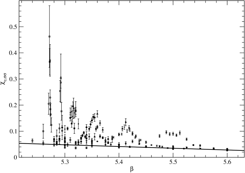
Figure 16: Specific heat curves. The thick line shows the best linear fit for the background.

The best fit is obtained excluding a region of width $12W$. Table 9 shows the stability of the fit as the parameter $n$ is in the range 6-15.

It should be noticed that even the $\beta$ dependence is very weak and that $C_{0}(\beta)$ is consistent with a constant in the $\beta$ range examined within the statistical errors so that the whole procedure described here is in practice equivalent to taking $C_{0}(\beta)$ a constant.

Table 9: $C_{0}(\beta)$ fit parameters for different values of $n$. The fit function is $C_{0}(\beta)=q_{1}+q_{2}\beta$

$n$	$q_{1}$	$q_{2}$	$\chi^{2}$/$d.o.f.$	$d.o.f.$
3	0.608(60)	-0.103(11)	8.70	84
4	0.535(44)	-0.0908(84)	5.17	77
5	0.529(48)	-0.0887(88)	5.19	66
6	0.452(44)	-0.0751(80)	3.56	58
7	0.444(44)	-0.0740(80)	3.62	53
8	0.436(44)	-0.0728(80)	3.61	47
9	0.416(44)	-0.0693(77)	3.19	42
10	0.420(44)	-0.0695(75)	3.11	37
11	0.401(41)	-0.0661(77)	2.89	34
12	0.400(43)	-0.0663(83)	2.81	29
13	0.405(53)	-0.0668(97)	2.99	26
14	0.411(56)	-0.068(10)	2.95	24
15	0.404(56)	-0.067(10)	3.15	21

References

- (1) A recent review on QCD thermodynamics is contained in: E. Laermann and O. Philipsen, Ann. Rev. Nucl. Part. Sci. 53 (2003) 163 [arXiv:hep-ph/0303042].
- (2) R. D. Pisarski and F. Wilczek, Phys. Rev. D 29, 338 (1984);
- (3) F. Wilczek, Int. J. Mod. Phys. A 7, 3911 (1992);
- (4) K. Rajagopal and F. Wilczek, Nucl. Phys. B 399, 395 (1993)
- (5) M. A. Stephanov, K. Rajagopal and E. V. Shuryak, Phys. Rev. Lett. 81 (1998) 4816 [arXiv:hep-ph/9806219].
- (6) M. Fukugita, H. Mino, M. Okawa and A. Ukawa, Phys. Rev. Lett. 65, 816 (1990).
- (7) M. Fukugita, H. Mino, M. Okawa and A. Ukawa, Phys. Rev. D 42, 2936 (1990).
- (8) F. R. Brown, F. P. Butler, H. Chen, N. H. Christ, Z. Dong, W. Schaffer, L. I. Unger and A. Vaccarino, Phys. Rev. Lett. 65, 2491 (1990)
- (9) F. Karsch, Phys. Rev. D 49, 3791 (1994).
- (10) F. Karsch and E. Laermann, Phys. Rev. D 50, 6954 (1994).
- (11) S. Aoki et al. (JLQCD collaboration), Phys. Rev. D 57, 3910 (1998) [arXiv:hep-lat/9710048].
- (12) C. Bernard, C. DeTar, S. Gottlieb, U. M. Heller, J. Hetrick, K. Rummukainen, R.L. Sugar and D. Toussaint, Phys.Rev. D 61, 054503 (2000)
- (13) A. A. Khan et al. (CP-PACS collaboration), Phys. Rev. D 63, 034502 (2001) [arXiv:hep-lat/0008011].
- (14) M. D’Elia, A. Di Giacomo and C. Pica, arXiv:hep-lat/0408008.
- (15) M.E. Fisher and M.N. Barber, Phys. Rev. Lett.28 1516 (1972)
- (16) E. Brézin, J. Physique 43 15 (1982)
- (17) S. A. Gottlieb, W. Liu, D. Toussaint, R. L. Renken and R. L. Sugar, Phys. Rev. D 35 (1987) 2531.
- (18) T. Blum et al. (MILC collaboration), Phys. Rev. D 51 5153 (1995).
- (19) M.E.J. Newman and G.T. Barkema, “Monte Carlo Methods in Stastical Physics”, Oxford University Press (1999)
- (20) F. Karsch, ILL-TH-86-9, Invited talk given at the Workshop on Lattice Gauge Theory - A Challenge in Large Scale Computing, Wuppertal, Germany, Nov 5-7, 1985