HISKP-TH-05/08, FZJ-IKP-TH-2005-11, TUM-T39-05-01

Abstract

We calculate the nucleon and the delta mass to fourth order in a covariant formulation of the small scale expansion. We analyze lattice data from the MILC collaboration and demonstrate that the available lattice data combined with our knowledge of the physical values for the nucleon and delta masses lead to consistent chiral extrapolation functions for both observables up to fairly large pion masses. This holds in particular for very recent data on the delta mass from the QCDSF collaboration. The resulting pion-nucleon sigma term is $\sigma_{\pi N}=48.9$ MeV. This first quantitative analysis of the quark-mass dependence of the structure of the $\Delta(1232)$ in full QCD within chiral effective field theory suggests that (the real part of) the nucleon-delta mass-splitting in the chiral limit, $\Delta_{0}=0.33\,$GeV, is slightly larger than at the physical point. Further analysis of simultaneous fits to nucleon and delta lattice data are needed for a precision determination of the properties of the first excited state of the nucleon.

1. The $\Delta(1232)$ is the most important baryon resonance. It is almost degenerate in mass with the nucleon and couples strongly to pions, nucleons and photons. It was therefore argued early that spin-3/2 (decuplet) states should be included in baryon chiral perturbation theory [2], which is the low-energy effective field theory of the Standard Model. In Ref.[2] and subsequent works use was made of the heavy baryon approach, which treats the baryons as static sources. However, due to the fact that the nucleon-delta mass splitting $\Delta=m_{\Delta}-m_{N}$ stays finite in the chiral limit and thus introduces an additional low energy scale, in chiral effective field theories (ChEFT) special care has to be taken about the decoupling of resonances in the chiral limit [3]. This requirement can be systematized by counting the nucleon-delta mass splitting as an additional small parameter [4], which ensures that at each order in the chiral expansion enough counterterms are present to guarantee decoupling and renormalization [5]. The corresponding power counting was called the “small scale expansion” (SSE) [4]. The heavy baryon approach has been successfully applied to a variety of processes, for reviews see [6, 7], and a status report on chiral effective field theories with deltas is given in [8]. More recently, it was realized that for certain considerations/processes a Lorentz-invariant formulation of baryon chiral perturbation theory is advantageous. A particularly elegant scheme to perform covariant calculations is the so–called “infrared regularization” (IR) of [9]. The renormalization of relativistic baryon chiral perturbation theory has been discussed in detail in [10]. In Ref.[11] we gave a consistent extension of the infrared regularization method in the presence of spin-3/2 fields. It was in particular shown that in the covariant formulation of the SSE the contribution of the non-propagating spin-1/2 components of the Rarita-Schwinger field can be completely absorbed in the polynomial terms stemming from the most general effective chiral Lagrangian, analogous to the situation in the non-relativistic SSE [4]. In this letter, we apply the covariant SSE formalism to the nucleon and the delta mass as well as the $\pi N$ sigma term. We perform a fourth order calculation in the small parameter $\varepsilon$, where $\varepsilon$ collects small external momenta, the pion mass and the $N\Delta$ mass splitting. These explicit representations of $m_{N}$ and $m_{\Delta}$ serve as chiral extrapolation functions to analyze lattice simulations for nucleon and delta masses involving dynamical fermions, as for example reported by the CPPACS [15] and JLQCD collaboration [16]. While a detailed (combined) analysis of these and forthcoming data [17] analogous to the work reported in Ref.[18] certainly also needs to take into account the observed finite volume dependences [15, 16], in this letter our aim is more modest. We attempt to connect the lattice data for nucleon and delta masses as reported by the MILC collaboration [20] with the known results at the physical point. The MILC data have the exciting feature that they cover unphysical pion masses as low as $M_{\pi}\simeq 350$ MeV on a relatively large lattice with $L=2.6$ fm, although there is still considerable discussion within the lattice QCD community about the technical details of the employed (staggered) fermion actions, see e.g. [21]. Clearly, such extrapolation functions based on chiral perturbation theory cease to make sense at too large values of the quark (pion) masses, but as we will demonstrate later, we can nicely capture the trend of these data. More lattice results also at lower pion masses are clearly needed, and these should be analyzed utilizing the (infinite volume) extrapolation functions given here.

2. Our calculations are based on the effective Lagrangian of nucleons and deltas coupled to external sources. The various contributions to S-matrix elements and transition currents are organized in powers of the small parameter $\varepsilon$, where $\varepsilon$ collectively denotes small pion four-momenta, the pion mass, baryon three momenta and the nucleon-delta splitting, $\Delta=m_{\Delta}-m_{N}$ (more precisely, the difference in the chiral limit). The expansion in powers of $\varepsilon$ is called the small scale expansion. In what follows, we will consider the nucleon and the delta mass to fourth order in the SSE. Consider first the pion-nucleon Lagrangian. The terms pertinent to the observables calculated here read (for details, see [5, 6, 24]),

$${\cal L}_{\pi N}^{(1)} = \bar{\psi}_{N}\left[i\not{\!\!D}-m_{0}+\frac{g_{A}}{2}\not{u}\gamma_{5}\right]\psi_{N}~{},$$ (1)

$${\cal L}_{\pi N}^{(2)} = \bar{\psi}_{N}\left[c_{1}\langle\chi_{+}\rangle-\frac{c_{2}}{4m_{0}^{2}}\left\{\langle u_{\mu}u_{\nu}\rangle D^{\mu}D^{\nu}+{\rm h.c.}\right\}+\frac{c_{3}}{2}\langle u^{2}\rangle+\ldots\right]\psi_{N}~{},$$ (2)

$${\cal L}_{\pi N}^{(3)} = \bar{\psi}_{N}\left\{B_{23}\,\Delta_{0}\,\langle\chi_{+}\rangle+B_{32}\,\Delta_{0}^{3}+...\right\}\psi_{N}~{},$$ (3)

$${\cal L}_{\pi N}^{(4)} = \bar{\psi}_{N}\left\{e_{38}\,\langle\chi_{+}\rangle^{2}+e_{115}\,\frac{1}{4}\langle\chi_{+}^{2}-\chi_{-}^{2}\rangle-e_{116}\,\frac{1}{4}\biggl{(}\langle\chi_{-}^{2}\rangle-\langle\chi_{-}\rangle^{2}+\langle\chi_{+}^{2}\rangle-\langle\chi_{+}\rangle^{2}\biggr{)}\right.$$ (4)

$$\qquad\qquad\qquad\qquad\qquad\qquad\left.+E_{1}\,\Delta_{0}^{4}+E_{2}\,\Delta_{0}^{2}\,\langle\chi_{+}\rangle+\ldots\right\}\psi_{N}~{}.$$

Here, $\psi_{N}$ denotes the nucleon spinor, $g_{A}$ is the axial-vector coupling constant (in the chiral limit), $m_{0}$ the chiral limit value of the nucleon mass, $\chi_{+}$ contains the external scalar fields which contains the quark mass matrix and $\langle\ldots\rangle$ denotes the trace in flavor space. The $c_{i}$ are low-energy constants (LECs). Their values can e.g. be determined in the analysis of pion-nucleon scattering in the delta-full EFT [25]. It is known that in particular $c_{2}$ and $c_{3}$ are largely saturated by $\Delta$-exchange [26], thus the remaining contributions in an EFT with explicit spin-3/2 fields are expected to be very small. The counterterms $B_{23},\,B_{32},\,E_{1},\,E_{2}$ in ${\mathcal{L}}_{\pi N}^{(3,4)}$ appear naturally in SSE ($\Delta_{0}\sim{\cal O}(\epsilon)$) and are required for the renormalization of the loop graphs at ${\cal O}(\epsilon^{3,4}$). Furthermore, their finite parts are chosen in such a way that in the limit $m_{\pi}/\Delta_{0}\rightarrow 0$ the ${\cal O}(\epsilon^{n})$ SSE result recovers the ${\cal O}(p^{n})$ result of heavy baryon chiral perturbation theory (HBCHPT). The fourth-order LECs $e_{i}$ contribute to the nucleon mass in the combination $e_{1}=16e_{38}+2e_{115}+e_{116}/2$ (for details, see [24, 22]). The relevant terms from the covariant $\pi N\Delta$ Lagrangian read [27]

$${\cal L}_{\pi N\Delta}^{(1)} = c_{A}\bar{\psi}^{i}_{\alpha}O^{\alpha\beta}_{A}w_{\beta}^{i}\psi_{N}+{\rm h.c.}~{},$$ (5)

$${\cal L}_{\pi N\Delta}^{(2)} = \bar{\psi}^{i}_{\alpha}O^{\alpha\mu}_{A}\left\{b_{3}\,i\,w_{\mu\nu}^{i}\,\gamma^{\nu}+\frac{b_{6}}{m_{0}}\,i\,w_{\mu\nu}^{i}\,i\,D^{\nu}+\ldots\right\}\psi_{N}+{\rm h.c.}~{},$$ (6)

with $w_{\mu}^{i}=\langle\tau^{i}u_{\mu}\rangle/2$ and $w_{\mu\nu}^{i}=\langle\tau^{i}\left[D_{\mu},u_{\nu}\right]\rangle/2$, where $\tau^{i},\,i=1,2,3$ denote the Pauli matrices in isospin space. The tensor $O_{\alpha\beta}^{A}=g_{\alpha\beta}+\frac{2\,A}{d}\gamma_{\alpha}\gamma_{\beta}$ takes care of the “point-invariance” of the spin-3/2 theory [4]. Here, ${\psi}_{i}^{\mu}$ denotes the spin-3/2 field in Rarita-Schwinger notation with an additional isospin-index $i$ and the constraint $\tau^{i}\,{\psi}_{i}^{\mu}=0$ [4]. The LEC $c_{A}$ represents the leading axial-vector $N\Delta$ coupling constant (frequently called $g_{\pi N\Delta}$ in the literature). At second order, we have two relevant couplings, parameterized by the LECs $b_{3}$ and $b_{6}$. We note that in the non-relativistic theory the leading contribution of $b_{6}$ can be absorbed in the coupling $b_{3}$ to ${\cal O}(\varepsilon^{2})$ [4]. In the non-relativistic SSE $b_{6}$ therefore only appears as an independent coupling at ${\cal O}(\varepsilon^{3})$ . Finally, we list the terms of the Lagrangian that describe the delta propagation and its coupling to pions and external sources. The pertinent covariant structures up to ${\cal O}(\varepsilon^{2})$ have been constructed in [27], here we add further terms needed up ${\cal O}(\varepsilon^{4})$ in close analogy to the nucleon case (see also [25]). Specifically, we employ

$${\cal L}_{\pi\Delta}^{(1)} = \!\!\!\!-\bar{\psi}_{\alpha}^{i}O^{\alpha\mu}_{A}\left\{\left[i\not{\!\!D}^{ij}-m_{\Delta}^{0}\xi^{ij}_{3/2}+\frac{g_{1}}{2}\!\!\not{\!\!u}^{ij}\gamma_{5}\right]g_{\mu\nu}-\frac{\gamma_{\mu}\gamma_{\lambda}}{4}\left(i\not{\!\!D}^{ij}-m_{\Delta}^{0}\xi^{ij}_{3/2}\right)\gamma^{\lambda}\gamma_{\nu}\right\}O^{\nu\beta}_{A}\psi_{\beta}^{j},$$ (7)

$${\cal L}_{\pi\Delta}^{(2)} = -\,\bar{\psi}_{\alpha}^{i}O^{\alpha\mu}_{A}\left\{\left[a_{1}\langle\chi_{+}\rangle\delta^{ij}-\frac{a_{2}}{4m_{0}^{2}}\left\{\langle u_{\alpha}u_{\beta}\rangle D^{\alpha}_{ik}D^{\beta}_{kj}+{\rm h.c.}\right\}\right.\right.$$ (8)

$$\left.\left.\quad\qquad\qquad\qquad\qquad\qquad+\frac{a_{3}}{2}\langle u^{2}\rangle\delta^{ij}+\ldots\right]g_{\mu\nu}+\ldots\right\}O^{\nu\beta}_{A}\psi_{\beta}^{j},$$

$${\cal L}_{\pi\Delta}^{(3)} = -\,\bar{\psi}_{\alpha}^{i}O^{\alpha\mu}_{A}\left\{B_{1}^{\Delta}\,\Delta_{0}\,\langle\chi_{+}\rangle+B_{0}^{\Delta}\,\Delta_{0}^{3}+\ldots\right\}g_{\mu\nu}\delta^{ij}O^{\nu\beta}_{A}\psi_{\beta}^{j}$$ (9)

$${\cal L}_{\pi\Delta}^{(4)} = -\,\bar{\psi}_{\alpha}^{i}O^{\alpha\mu}_{A}\left\{e_{38}^{\Delta}\,\langle\chi_{+}\rangle^{2}+e_{115}^{\Delta}\,\frac{1}{4}\langle\chi_{+}^{2}-\chi_{-}^{2}\rangle-e_{116}^{\Delta}\,\frac{1}{4}\biggl{(}\langle\chi_{-}^{2}\rangle-\langle\chi_{-}\rangle^{2}+\langle\chi_{+}^{2}\rangle-\langle\chi_{+}\rangle^{2}\biggr{)}\right.$$ (10)

$$\left.\quad\qquad\qquad\qquad\qquad+E_{1}^{\Delta}\,\Delta_{0}^{4}+E_{2}^{\Delta}\,\Delta_{0}^{2}\,\langle\chi_{+}\rangle+\ldots\right\}g_{\mu\nu}\delta^{ij}O^{\nu\beta}_{A}\psi_{\beta}^{j}$$

with $D_{\mu}^{ij}=D_{\mu}\delta^{ij}-i\epsilon^{ijk}\,\langle\tau^{k}D_{\mu}\rangle$, $u_{\mu}^{ij}=u_{\mu}\delta^{ij}$ and $\xi^{ij}_{3/2}$ denotes the isospin 3/2 projector, $\xi^{ij}_{3/2}=\delta^{ij}-\tau^{i}\tau^{j}/3$. Further, $g_{1}$ denotes the axial $\Delta\Delta$ coupling constant (in the chiral limit), whereas $m_{\Delta}^{0}$ refers to the $\Delta$(1232) mass (in the chiral limit). The LECs $a_{i}$ correspond to the $c_{i}$ in Eq. (2) and so on. The $B_{i}^{\Delta}$ and $E_{i}^{\Delta}$ are taken such that the values of $m_{0}^{\Delta}$ and $a_{1}$ in the chiral limit are not affected by loop corrections.

3. Choosing $A=-1$ the propagator for a spin-3/2–isospin-3/2 particle in the Rarita-Schwinger formalism has the general form

$$S_{\mu\nu}^{ij}(p) = -i\,\frac{\not{p}+m_{\Delta}^{0}}{p^{2}-(m_{\Delta}^{0})^{2}}\,\left[g_{\mu\nu}-{1\over d-1}\,\gamma_{\mu}\gamma_{\nu}-{(d-2)\,p_{\mu}p_{\nu}\over(d-1)\,(m_{\Delta}^{0})^{2}}+{p_{\mu}\gamma_{\nu}-p_{\nu}\gamma_{\mu}\over(d-1)\,m_{\Delta}^{0}}\right]\,\xi^{ij}_{3/2}\;.$$ (11)

The Dirac-tensor $S_{\mu\nu}$ can be written as a linear superposition of spin-3/2 and spin-1/2 projection operators $P_{\mu\nu}^{3/2},\,P_{\mu\nu}^{1/2}$:

$$-i\,S_{\mu\nu}^{\Delta}(p) = -{\not{p}+m_{\Delta}^{0}\over p^{2}-(m_{\Delta}^{0})^{2}}\,P_{\mu\nu}^{3/2}-{1\over\sqrt{d-1}m_{\Delta}^{0}}\Biggl{(}\bigl{(}P_{12}^{1/2}\bigr{)}_{\mu\nu}+\bigl{(}P_{21}^{1/2}\bigr{)}_{\mu\nu}\Biggr{)}$$ (12)

$$\quad+{d-2\over(d-1)\,(m_{\Delta}^{0})^{2}}\,(\not{p}+m_{\Delta}^{0})\,\bigl{(}P_{22}^{1/2}\bigr{)}_{\mu\nu}~{}.$$

For details regarding the properties of the projectors we refer to [11]. As can be clearly seen from Eq.(12) only the spin-3/2 components are associated with a propagation, whereas the (spurious) spin-1/2 components correspond to local contact operators. Given that the chiral effective field theory for a coupled nucleon-delta system contains the most general set of local contact operators allowed by chiral symmetry, it was argued in [11] that in chiral EFT one only needs to take into account the propagation of the spin-3/2 degrees of freedom. The effects of the spurious/off-shell spin-1/2 components are already completely accounted for by the counterterms of the theory. In [11] we have therefore proposed to utilize the propagator form A

$$G_{\mu\nu}^{ij}|_{\rm IR}^{A}(p) = -i\,\frac{\not{p}+m_{\Delta}^{0}}{p^{2}-(m_{\Delta}^{0})^{2}}\,P_{\mu\nu}^{3/2}\,\xi^{ij}_{3/2}\;,$$ (13)

with the spin-3/2 projector

$$P_{\mu\nu}^{3/2} = g_{\mu\nu}-\frac{1}{d-1}\,\gamma_{\mu}\gamma_{\nu}-\frac{1}{(d-1)\,p^{2}}\left(\not{p}\gamma_{\mu}p_{\nu}+p_{\mu}\gamma_{\nu}\not{p}\right)-\frac{(d-4)}{(d-1)}\,\frac{p_{\mu}p_{\nu}}{p^{2}}~{}.$$ (14)

In the meantime it was realized in practical applications that it is advantageous to use a different form for the propagator than the one given in Eq.(13) (see also the related work in [32]). In Ref.[11] it was shown that due to the extra $1/p^{2}$ structure in Eq.(14) the standard rules of infrared regularization had to be modified for a consistent treatment of the low-energy modes, making loop-calculations in this covariant field theory more tedious. Here we propose another separation of the general Dirac-tensor:

$$S_{\mu\nu}^{\Delta} = -i\,\frac{\not{p}+m_{\Delta}^{0}}{p^{2}-(m_{\Delta}^{0})^{2}}\,\frac{p^{2}}{(m_{\Delta}^{0})^{2}}\,P_{\mu\nu}^{3/2}+i\,R_{\mu\nu}$$ (15)

Once more it can be shown that the remainder

$$R_{\mu\nu} = \frac{\not{p}+m_{\Delta}^{0}}{(m_{\Delta}^{0})^{2}}\left[g_{\mu\nu}-\frac{1}{d-1}\,\gamma_{\mu}\gamma_{\nu}\right]+\frac{1}{(d-1)\,(m_{\Delta}^{0})^{2}}\left[p_{\mu}\gamma_{\nu}-\gamma_{\mu}p_{\nu}\right]$$ (16)

is not connected with the spin-3/2 propagation, that it is local and that it cannot generate any contributions which are not already contained in the counterterms of the effective field theory. As an alternative to Eq.(13) we therefore propose the propagator form

$$G_{\mu\nu}^{ij}|_{\rm IR}^{B}(p) = -i\,\frac{\not{p}+m_{\Delta}^{0}}{p^{2}-(m_{\Delta}^{0})^{2}}\,\frac{p^{2}}{(m_{\Delta}^{0})^{2}}\,P_{\mu\nu}^{3/2}\,\xi^{ij}_{3/2}\;.$$ (17)

We note that in form B there is no more $1/p^{2}$ structure, making the evaluation of loop diagrams containing spin-3/2 degrees of freedom in the IR-scheme a lot simpler. However, we emphasize that in a low-energy (chiral) effective field theory the finite/renormalized results obtained via Eq.(13) or Eq.(17) are identical—it is merely a matter of practicability which method is chosen for a particular observable. In what follows, we will work with form B. We note explicitly that one could also work with the full Rarita-Schwinger propagator of Eq.(11), however, form A or form B have the advantage that the results can be directly mapped to the known couplings of the heavy-baryon formulation of SSE where also only the spin-3/2 components are part of the propagator [2, 4]. Finally we remark that for low energies the width of $\Delta(1232)$ can be treated perturbatively in the covariant SSE, analogous to the situation in the non-relativistic theory. Throughout this work we will therefore not address this issue, applications of the covariant SSE in the resonance region will be discussed in a forthcoming paper [29].

4. Armed with the effective Lagrangian, we are now in the position to calculate the nucleon and the delta self-energy to fourth order in the covariant SSE. The covariant formalism allows in particular to resum the contributions from kinetic energy insertions. The nucleon mass can be written as

$$m=m_{0}-4c_{1}M_{\pi}^{2}-4M_{\pi}^{2}\Delta_{0}B_{23}-B_{32}\Delta_{0}^{3}-4e_{1}(\lambda)M_{\pi}^{4}-E_{1}\Delta_{0}^{4}-4M_{\pi}^{2}\Delta_{0}^{2}E_{2}+m^{{\rm N-loop}}+m^{{\rm\Delta-loop}}~{},$$ (18)

with the corresponding fourth-order tree and one-loop graphs shown in Fig. 1. The contributions from the nucleon and delta loop graphs, which start at ${\mathcal{O}}(\varepsilon^{3})$, take the form

$$m^{{\rm N-loop}} = -\frac{3g_{A}^{2}}{2F_{\pi}^{2}}m_{0}M_{\pi}^{2}I_{11}^{(0,0)}(m_{0}^{2},m_{0}^{2})-\frac{3M_{\pi}^{2}}{F_{\pi}^{2}}\left(-2c_{1}+\frac{c_{2}}{d}+c_{3}\right)\Delta_{\pi}~{},$$ (19)

$$m^{{\rm\Delta-loop}} = \frac{2c_{A}^{2}\,(d-2)}{F_{\pi}^{2}}\frac{m_{0}^{2}}{(m_{\Delta}^{0})^{2}}\,\left\{\left(m+m_{\Delta}^{0}\right)I_{11}^{(2,0)}(m_{0}^{2},(m_{\Delta}^{0})^{2})-m_{0}I_{11}^{(3,1)}(m_{0}^{2},(m_{\Delta}^{0})^{2})\right\}$$ (20)

$$- b_{3}\frac{c_{A}}{2F_{\pi}^{2}(m_{\Delta}^{0})^{2}}\frac{d-2}{d-1}\biggl{\{}\biggl{[}-(m_{0}^{2}-(m_{\Delta}^{0})^{2})^{2}+M_{\pi}^{2}\biggl{(}4\frac{d-1}{d}m_{0}^{2}-4\frac{m_{0}m_{\Delta}^{0}}{d}+M_{\pi}^{2}\biggl{)}\biggr{]}\Delta_{\pi}$$

$$- \bigl{[}(m_{0}^{2}-(m_{\Delta}^{0})^{2})^{2}+M_{\pi}^{2}(M_{\pi}^{2}-2(m_{0}^{2}+(m_{\Delta}^{0})^{2}))\bigr{]}$$

$$\times \biggl{[}(m_{0}^{2}-(m_{\Delta}^{0})^{2}-M_{\pi}^{2})I_{11}^{(0,0)}(m_{0}^{2},(m_{\Delta}^{0})^{2})+2m_{0}m_{\Delta}^{0}I_{11}^{(1,1)}(m_{0}^{2},(m_{\Delta}^{0})^{2})\biggr{]}\biggr{\}}$$

$$- \frac{b_{6}}{m_{0}}\frac{c_{A}}{2F_{\pi}^{2}(m_{\Delta}^{0})^{2}}\biggl{\{}\biggl{[}-(m_{0}^{2}-(m_{\Delta}^{0})^{2})^{2}+M_{\pi}^{2}\biggl{(}2\frac{d-2}{d}m_{0}^{2}+2(m_{\Delta}^{0})^{2}\biggr{)}-M_{\pi}^{2}](m_{0}+m_{\Delta}^{0})$$

$$- \frac{2}{d}M_{\pi}^{2}m_{0}(-2M_{\pi}^{2}-m_{0}^{2}+(m_{\Delta}^{0})^{2})\biggr{]}\Delta_{\pi}-\bigl{[}(m_{0}^{2}-(m_{\Delta}^{0})^{2})^{2}+M_{\pi}^{2}(M_{\pi}^{2}-2(m_{0}^{2}+(m_{\Delta}^{0})^{2})$$

$$\times (m_{0}^{2}-(m_{\Delta}^{0})^{2}+M_{\pi}^{2})((m_{0}+m_{\Delta}^{0})I_{11}^{(0,0)}(m_{0}^{2},(m_{\Delta}^{0})^{2})-m_{0}I_{11}^{(1,1)}(m_{0}^{2},(m_{\Delta}^{0})^{2})\bigr{]}\biggr{\}}~{}.$$

Here, $F_{\pi}$ is the pion decay constant and $\lambda$ the scale of dimensional regularization. Throughout, we set $\lambda=1.232$ GeV.

Figure 1: Fourth order contributions to the nucleon (left panel) and the delta mass (right panel). Solid, double and dashed lines denote nucleons, deltas and pions, in order. The corresponding dimension two $(a_{i},b_{i},c_{i})$ and four ($e_{i}$) LECs are also given at the pertinent vertices.

The loop functions which appear here and for the delta mass discussed below are defined as:

$$\frac{1}{i}\int d^{4}k\{1,k_{\mu},k_{\mu}k_{\nu},k_{\mu}k_{\nu}k_{\rho}\}\frac{1}{(M_{\pi}^{2}-k^{2})(m^{2}-(p-k)^{2})}=\biggl{\{}H_{11}^{(0,0)}(p^{2},m^{2})\ ,$$

$$p_{\mu}H_{11}^{(1,1)}(p^{2},m^{2}),g_{\mu\nu}H_{11}^{(2,0)}(p^{2},m^{2})+\ldots,(p_{\rho}g_{\mu\nu}+p_{\mu}g_{\rho\nu}+p_{\nu}g_{\mu\rho}H_{11}^{(3,1)}(p^{2},m^{2})+\ldots\biggr{\}}~{}.$$ (21)

Their irregular parts are given by:

$$I_{11}^{(0,0)}(p^{2},m^{2})=-\frac{p^{2}-m^{2}+M_{\pi}^{2}}{2p^{2}}\frac{1}{16\pi^{2}}\left({\ln}\frac{M_{\pi}^{2}}{p^{2}}-1\right)-\bar{J}_{0}$$ (22)

with

$$\bar{J}_{0}=\frac{1}{32\pi^{2}p^{2}}\ \sqrt{\lambda(p^{2},m^{2},M_{\pi}^{2})}\ {\ln}\frac{p^{2}-m^{2}+M_{\pi}^{2}+\sqrt{\lambda(p^{2},m^{2},M_{\pi}^{2})}}{p^{2}-m^{2}+M_{\pi}^{2}-\sqrt{\lambda(p^{2},m^{2},M_{\pi}^{2})}}+i\frac{\sqrt{\lambda(p^{2},m^{2},M_{\pi}^{2})}}{16\pi p^{2}}~{},$$ (23)

if $\lambda(p^{2},m^{2},M_{\pi}^{2})>0$. Otherwise, we have

$$\bar{J}_{0}=\frac{1}{16\pi^{2}p^{2}}\ \sqrt{-\lambda(p^{2},m^{2},M_{\pi}^{2})}\ \ {\arccos}\left(-\frac{p^{2}-m^{2}+M_{\pi}^{2}}{2M_{\pi}\sqrt{p^{2}}}\right)~{}.$$ (24)

The other relevant loop functions can be expressed as

$$I_{11}^{(1,1)}(p^{2},m^{2}) = \frac{1}{2p^{2}}\biggl{(}(p^{2}-m^{2}+M_{\pi}^{2})I_{11}^{(0,0)}+\frac{1}{2}\Delta_{\pi}\biggr{)}~{},$$ (25)

$$I_{11}^{(2,0)}(p^{2},m^{2}) = \frac{1}{4(d-1)p^{2}}\biggl{(}\lambda(p^{2},m^{2},M_{\pi}^{2})I_{11}^{(0,0)}-(p^{2}-m^{2}+M_{\pi}^{2})\Delta_{\pi}\biggr{)}~{},$$ (26)

$$I_{11}^{(3,1)}(p^{2},m^{2}) = \frac{1}{2p^{2}}\biggl{(}(p^{2}-m^{2}+M_{\pi}^{2})I_{11}^{(2,0)}+\frac{M_{\pi}^{2}}{d}\Delta_{\pi}\biggr{)}~{}.$$ (27)

We also employ the standard definition of $\Delta_{\pi}$,

$$\Delta_{\pi}=\frac{1}{i}\int\frac{d^{d}k}{(2\pi)^{d}}\frac{1}{M_{\pi}^{2}-k^{2}}~{}.$$ (28)

Using these, the $\Delta$-loop contribution can be written as an infinite series in $M_{\pi}$ (modulo chiral $\log$s):

$$m_{N}^{\rm\Delta-loop}=l_{0}+l_{1}\,M_{\pi}^{2}+l_{2}\,M_{\pi}^{4}+\ldots~{},$$ (29)

with $l_{0},l_{1}$ being infinite series in $\Delta_{0}$ starting at ${\mathcal{O}}(\varepsilon^{3})$ and ${\mathcal{O}}(\varepsilon)$, respectively. Note that the decoupling theorem is automatically fulfilled here since there is no nonanalytic contribution $\sim M_{\pi}^{3}$. Now as a minimal way of determining the LECs $B_{23}$, $B_{32}$, $E_{1}$ and $E_{2}$ one can choose $B_{23}+\Delta_{0}^{2}E_{2}=l_{1}/4$, and $B_{32}+\Delta_{0}E_{1}=l_{0}/4$, which means that the $\Delta$ contribution will first occur at order $M_{\pi}^{4}$.

The chiral expansion of the delta mass can be written in a way similar to the case of the nucleon Eq. (18) (the corresponding tree and loop graphs that contribute at ${\cal O}(\varepsilon^{4})$ are collected in Fig. 1),

$$m_{\Delta}=m_{\Delta}^{0}-4a_{1}M_{\pi}^{2}-4M_{\pi}^{2}\Delta_{0}B_{1}^{\Delta}-B_{0}^{\Delta}\Delta_{0}^{3}-4e_{1}^{\Delta}(\lambda)M_{\pi}^{4}-E_{1}^{\Delta}\Delta_{0}^{4}-4M_{\pi}^{2}\Delta_{0}^{2}E_{2}^{\Delta}+m_{\Delta}^{{\rm N-loop}}+m_{\Delta}^{{\rm\Delta-loop}}~{},$$ (30)

with

$$m_{\Delta}^{{\rm N-loop}} = \frac{c_{A}^{2}}{F_{\pi}^{2}}\,\left\{\left(m_{\Delta}^{0}+m_{0}\right)I_{11}^{(2,0)}((m_{\Delta}^{0})^{2},m_{0}^{2})-m_{\Delta}^{0}I_{11}^{(3,1)}((m_{\Delta}^{0})^{2},m_{0}^{2})\,\right\}$$ (31)

$$+ b_{3}\frac{c_{A}}{F_{\pi}^{2}}\frac{M_{\pi}^{2}}{d}\biggl{\{}\Delta_{\pi}+[(m_{\Delta}^{0})^{2}-m_{0}^{2}-M_{\pi}^{2}]I_{11}^{(0,0)}((m_{\Delta}^{0})^{2},m_{0}^{2})+2m_{0}m_{\Delta}^{0}I_{11}^{(1,1)}((m_{\Delta}^{0})^{2},m_{0}^{2})\biggr{\}}$$

$$+ \frac{b_{6}}{m_{0}}\frac{c_{A}}{F_{\pi}^{2}}\frac{M_{\pi}^{2}}{d}\biggl{\{}\Delta_{\pi}(m_{0}+m_{\Delta}^{0})+[(m_{\Delta}^{0})^{2}-m_{0}^{2}+M_{\pi}^{2}]$$

$$\times \biggl{[}(m_{0}+m_{\Delta}^{0})I_{11}^{(0,0)}((m_{\Delta}^{0})^{2},m_{0}^{2})-m_{\Delta}^{0}I_{11}^{(1,1)}((m_{\Delta}^{0})^{2},m_{0}^{2})\biggr{]}\biggr{\}}$$

and

$$m_{\Delta}^{{\rm\Delta-loop}} = -\frac{5h_{A}^{2}}{6(m_{\Delta}^{0})^{2}F_{\pi}^{2}}\,\left\{m_{\Delta}^{0}\biggl{[}M_{\pi}^{2}\Delta_{\pi}\biggl{(}1-\frac{4}{d(d-1)}\biggr{)}-M_{\pi}^{2}(m_{\Delta}^{0})^{2}I_{11}^{(0,0)}((m_{\Delta}^{0})^{2},(m_{\Delta}^{0})^{2})\right.$$ (32)

$$+ \frac{1}{d-1}(4(m_{\Delta}^{0})^{2}+(d-4)M_{\pi}^{2})I_{11}^{(2,0)}((m_{\Delta}^{0})^{2},(m_{\Delta}^{0})^{2})\biggr{]}+m_{\Delta}^{0}\biggl{[}\frac{4}{d-1}(m_{\Delta}^{0})^{2}I_{11}^{(3,1)}((m_{\Delta}^{0})^{2},(m_{\Delta}^{0})^{2})\bigr{.}$$

$$- \left.\bigl{.}\frac{M_{\pi}^{2}}{d}\Delta_{\pi}\biggr{]}-\frac{1}{d(d-1)}M_{\pi}^{2}\Delta_{\pi}\right\}-\frac{3M_{\pi}^{2}}{F_{\pi}^{2}}\left(-2a_{1}+\frac{A}{d}+B\right)\Delta_{\pi}~{},$$

with $A=a_{2}+\dots$ and $B=a_{3}+\ldots$. It can easily be verified that $m_{\Delta}^{{\rm\Delta-loop}}$ starts as $M_{\pi}^{3}$ whereas, as in the case of the nucleon mass, $m_{\Delta}^{\rm N-loop}$ has a constant and a piece $\sim M_{\pi}^{2}$:

$$m_{\Delta}^{\rm N-loop}=l_{0}+l_{1}M_{\pi}^{2}+l_{2}M_{\pi}^{4}+\cdots$$ (33)

As before, we will choose $B_{0}^{\Delta}$, $B_{1}^{\Delta}$, $E_{1}^{\Delta}$ $E_{2}^{\Delta}$ in such a way that $m_{\Delta}^{\rm N-loop}$ starts to contribute only at $M_{\pi}^{4}$, that is $B_{0}^{\Delta}+\Delta_{0}^{2}E_{2}^{\Delta}=l_{1}/4$ and $B_{1}^{\Delta}+\Delta_{0}E_{2}^{\Delta}=l_{0}/4$. Note that we did not take into account the difference between the chiral limit value of the pion mass and its physical value [33]. This effect is known to be small, see e.g. the three-flavor calculation [23].

5. We are now in the position to analyze the nucleon and delta mass formulae given in Eqs. (18,30). They contain a certain number of LECs, some of which are (not very accurately) known from the study of pion-nucleon scattering in the heavy baryon SSE [25]. Here our aim is modest: In addition to the known values at the physical point we take the data from MILC [20] for the nucleon and the delta as function of the pion mass and try to describe these with LECs of natural size. Such a description is indeed possible, as shown in Fig. 2. So we do not intend detailed least-square fits here but rather try to find out whether the existing data shown in the this figure can be consistently described by our mass formulas with LECs of natural size. We stress again that a more refined analysis of e.g. pion-nucleon scattering in the covariant SSE is mandatory to put stringent constraints on certain combinations of the LECs (see also the extensive discussion in Refs.[22, 34] on this issue).

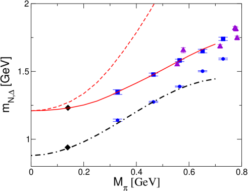
Figure 2: The nucleon mass (dot-dashed line) and the (real part of the) delta mass (solid line) as a function of the pion mass. The filled diamonds denote their physical values at the physical pion mass. The dashed line is the chiral extrapolation for the $\Delta$ based on SU(6) as explained in the text. The filled squares and circles are the MILC data [20]. The filled triangles are the recent data from QCDSF [17].

We have 11 (combinations of) parameters to determine, these are $c_{1},c_{2}/4+c_{3},a_{1},e_{1},e_{1}^{\Delta},c_{A},h_{A},b_{3},b_{6},A/4+B$ and $\Delta_{0}$. (i) constrained parameters: $c_{A}$ and $\Delta_{0}$ are fixed from the mass and width of the delta. We note that the $N\Delta$ mass splitting in the chiral limit, $\Delta_{0}=0.33\,$GeV, indicates a slightly larger $N\Delta$ mass splitting in the chiral limit than at the physical point. A similar observation was made in the case of quenched QCD, see [14] (for discussion about the difference between the mass splitting in the quenched approximation and full QCD, see also [35]). The LECs from the pion-nucleon Lagrangian, Eqs. (2,4) can be estimated from pion-nucleon scattering in the presence of the delta. We use $c_{1}=-0.8\,$GeV^-1 (which is within the uncertainty of the values determined in e.g. [36]) and $e_{1}=c_{2}=0$, $c_{3}=0.5\,$GeV^-1. The small values of $c_{2,3}$ are consistent with resonance saturation studies of [26] and the fits in [25]. (ii) Fit parameters: The remaining parameters are fit to the masses. We find for the two axial dimension two $N\Delta$ LECs the values $b_{3}=0.75$ GeV^-1 and $b_{6}=-0.75$. The axial $\Delta\Delta$ coupling is found to be $h_{A}=2$, which is not far from the SU(6) or large-$N_{C}$ value $h_{A}=9g_{A}/5=2.28$. Furthermore we get $e_{1}^{\Delta}=-1\,$GeV^-3, $a_{1}=-0.3\,$GeV^-1, $A=0$ and $B=0.5\,$GeV^-1. These are all natural values. It is interesting to note that $a_{1}$ is markedly smaller than $c_{1}$, although both couplings should be equal in the SU(6) limit. We refrain here from a detailed study of the theoretical errors that will be given in a forthcoming publication. Still, it is interesting to study the strict SU(6) limit. In that case, one would have $a_{1}=c_{1}=-0.8\,$GeV^-1 and $h_{A}=2.28$. As can be seen from the dashed line in Fig. 2, the assumption of strict SU(6) symmetry is clearly at odds with the MILC data, indicating that $a_{1}$ and $c_{1}$ indeed seem to have different values. Also shown in Fig. 2 are the recent QCDSF data for $m_{\Delta}$, which were not used in the fit but are nicely consistent with our extrapolation function. Note also that the QCDSF data are based on two-flavor simulations and are not very different from the MILC data in the region of overlap. This further supports our assumption on the treatment of the MILC data. We stress again that the resulting values of the LECs are to be considered indicative and a more analysis employing also contraints from other physical processes should follow.

From the small value of the LEC $a_{1}$ one immediately deduces that the $\pi\Delta$ sigma term appears to be significantly smaller than its nucleon cousin because at leading order in the quark mass expansion we have $\sigma_{\pi N}=-4c_{1}M_{\pi}^{2}+...$ and $\sigma_{\pi\Delta}=-4a_{1}M_{\pi}^{2}+...$. It is clear that this interesting observation deserves further study. Finally we note that the sigma term for the nucleon resulting from this “rough” fit is found as

$$\sigma_{\pi N}=48.9~{}{\rm MeV}~{},$$ (34)

to order $\varepsilon^{4}$. We note that this value is consistent with the classical result of Ref. [37], which was confirmed in [36] in a HBCHPT analysis of pion-nucleon scattering and in [34] in a ChEFT analysis of lattice data in a formalism without explicit delta degrees of freedom. It is also in agreement with the recent CHPT analysis of the three–flavor MILC data, see [23]. For the $\pi\Delta$ sigma term we get $\sigma_{\pi\Delta}=20.6\,$MeV. Again, these results need to be refined and bolstered by more detailed precise fits to the lattice data including also error and correlation analysis including also lattice data on other observables - the mass data alone are not sufficient to precisely pin down all parameters. Such an analysis, however, goes beyond the scope of this paper.

6. In this letter, we have presented a covariant extension of the small scale expansion, extending our earlier work [11]. We have analyzed the nucleon and the delta mass in view of the lattice data from MILC. These data seem to indicate sizeable SU(6) breaking effects that can be interpreted as a reduced pion cloud contribution in the resonance field (the delta) as compared to its ground-state (the nucleon). Our results obtained from fits to full QCD lattice data further indicate that the $N\Delta$ mass splitting can be larger in the chiral limit than at the physical point, analogous to observations in quenched QCD. We have also calculated the pion-nucleon sigma term and found good agreement with earlier determination from pion-nucleon scattering and the analysis of SU(2) and SU(3) lattice data for the nucleon. The recent QCDSF data for $m_{\Delta}$ are also consistent with our chiral extrapolation. It would be very valuable to have more (2 flavor) lattice results for the delta preferably at small pion masses to further sharpen these conclusions.

Acknowledgements

TRH acknowledges helpful discussions with G. Schierholz. We also thank G. Schierholz for providing us with QCDSF data prior to publication. TRH is grateful for the hospitality of the LPT at Université Louis Pasteur, Strasbourg, where a large part of this work was completed.

References

• [1]
• [2] E. Jenkins and A. V. Manohar, Phys. Lett. B 259 (1991) 353.
• [3] J. Gasser and A. Zepeda, Nucl. Phys. B 174 (1980) 445.
• [4] T. R. Hemmert, B. R. Holstein and J. Kambor, J. Phys. G 24 (1998) 1831 [arXiv:hep-ph/9712496].
• [5] V. Bernard, H. W. Fearing, T. R. Hemmert and U.-G. Meißner, Nucl. Phys. A 635 (1998) 121 [Erratum-ibid. A 642 (1998) 563] [arXiv:hep-ph/9801297].
• [6] V. Bernard, N. Kaiser and U.-G. Meißner, Int. J. Mod. Phys. E 4 (1995) 193 [arXiv:hep-ph/9501384].
• [7] U.-G. Meißner, in Shifman, M. (ed.): “At the frontier of particle physics”, vol. 1, pp. 417-505 (World Scientific, Singapore, 2001) [arXiv:hep-ph/0007092].
• [8] T. R. Hemmert, in Proceedings of NSTAR 01, Mainz, Germany; Eds. D. Drechsel and L. Tiator, World Scientific (Singapore) 2002. [arXiv:nucl-th/0105051].
• [9] T. Becher and H. Leutwyler, Eur. Phys. J. C 9 (1999) 643 [arXiv:hep-ph/9901384].
• [10] T. Fuchs, J. Gegelia, G. Japaridze and S. Scherer, Phys. Rev. D 68 (2003) 056005 [arXiv:hep-ph/0302117].
• [11] V. Bernard, T. R. Hemmert and Ulf-G. Meißner, Phys. Lett. B 565 (2003) 137 [arXiv:hep-ph/0303198].
• [12] B. C. Tiburzi and A. Walker-Loud, arXiv:hep-lat/0501018.
• [13] D. B. Leinweber, A. W. Thomas, K. Tsushima and S. V. Wright, Nucl. Phys. Proc. Suppl.  83, 179 (2000). [arXiv:hep-lat/9909109].
• [14] J. M. Zanotti, D. B. Leinweber, W. Melnitchouk, A. G. Williams and J. B. Zhang, arXiv:hep-lat/0407039.
• [15] A. Ali Khan et al. [CP-PACS Collaboration], Phys. Rev. D 65 (2002) 054505 [Erratum-ibid. D 67 (2003) 059901] [arXiv:hep-lat/0105015].
• [16] S. Aoki et al. [JLQCD Collaboration], Phys. Rev. D 68 (2003) 054502 [arXiv:hep-lat/0212039].
• [17] G. Schierholz, private communication; QCDSF collaboration, in preparation.
• [18] A. Ali Khan et al. [QCDSF-UKQCD Collaboration], Nucl. Phys. B 689 (2004) 175 [arXiv:hep-lat/0312030].
• [19] U.-G. Meißner, plenary talk at BARYONS 2004, Paris, France [arXiv:hep-ph/0501009], to appear in Nucl. Phys. A; T.R. Hemmert, in proceedings of the 337th WE-Heraeus seminar on Effective Field Theories in Nuclear, Particle and Atomic Physics (EFT04), J. Bijnens, U.-G. Meißner and A. Wirzba (eds.), Bad Honnef, Germany [arXiv:hep-ph/0502008].
• [20] C. W. Bernard et al., Phys. Rev. D 64, 054506 (2001) [arXiv:hep-lat/0104002].
• [21] S. Hashimoto, arXiv:hep-ph/0411126.
• [22] V. Bernard, T. R. Hemmert and U.-G. Meißner, Nucl. Phys. A 732 (2004) 149 [arXiv:hep-ph/0307115].
• [23] M. Frink, U.-G. Meißner and I. Scheller, arXiv:hep-lat/0501024, Eur. Phys. J. A (2005) 395.
• [24] N. Fettes, U.-G. Meißner, M. Mojžiš and S. Steininger, Annals Phys.  283 (2000) 273 [Erratum-ibid.  288 (2001) 249] [arXiv:hep-ph/0001308].
• [25] N. Fettes and Ulf-G. Meißner, Nucl. Phys. A 679 (2001) 629 [arXiv:hep-ph/0006299].
• [26] V. Bernard, N. Kaiser and Ulf-G. Meißner, Nucl. Phys. A 615 (1997) 483 [arXiv:hep-ph/9611253].
• [27] T. R. Hemmert, Ph.D. thesis, University of Massachusetts at Amherst (1997) [UMI-98-09346-mc].
• [28] K. Johnson and E. C. G. Sudarshan, Annals Phys.  13 (1961) 126.
• [29] V. Bernard, T. R. Hemmert and Ulf-G. Meißner, forthcoming.
• [30] R. F. Dashen, E. Jenkins and A. V. Manohar, Phys. Rev. D 49 (1994) 4713 [Erratum-ibid. D 51 (1995) 2489] [arXiv:hep-ph/9310379].
• [31] V. Pascalutsa and D. R. Phillips, Phys. Rev. C 67 (2003) 055202 [arXiv:nucl-th/0212024].
• [32] M. R. Schindler, J. Gegelia and S. Scherer, Phys. Lett. B 586 (2004) 258 [arXiv:hep-ph/0309005].
• [33] A. Fuhrer, Diploma Thesis “The nucleon in finite volume”, university of Berne (2004).
• [34] M. Procura, T. R. Hemmert and W. Weise, Phys. Rev. D 69 (2004) 034505 [arXiv:hep-lat/0309020].
• [35] R. D. Young, D. B. Leinweber, A. W. Thomas and S. V. Wright, Phys. Rev. D 66 (2002) 094507 [arXiv:hep-lat/0205017].
• [36] P. Büttiker and U.-G. Meißner, Nucl. Phys. A 668 (2000) 97 [arXiv:hep-ph/9908247].
• [37] J. Gasser, H. Leutwyler and M. E. Sainio, Phys. Lett. B 253 (1991) 252.