Finite-Size Effects in Lattice QCD with Dynamical Wilson Fermions

Abstract

As computing resources are limited, choosing the parameters for a full Lattice QCD simulation always amounts to a compromise between the competing objectives of a lattice spacing as small, quarks as light, and a volume as large as possible. Aiming to push unquenched simulations with the Wilson action towards the computationally expensive regime of small quark masses we address the question whether one can possibly save computing time by extrapolating results from small lattices to the infinite volume, prior to the usual chiral and continuum extrapolations. In the present work the systematic volume dependence of simulated pion and nucleon masses is investigated and compared with a long-standing analytic formula by Lüscher and with results from Chiral Perturbation Theory (ChPT). We analyze data from Hybrid Monte Carlo simulations with the standard (unimproved) two-flavor Wilson action at two different lattice spacings of $a\approx$ 0.08 fm and 0.13 fm. The quark masses considered correspond to approximately 85 and 50% (at the smaller $a$) and 36% (at the larger $a$) of the strange quark mass. At each quark mass we study at least three different lattices with $L/a=$10 to 24 sites in the spatial directions ($L=$0.85–2.08 fm).

I Introduction

It is in the nature of any numerical Lattice QCD calculation that it can only be done at non-zero lattice spacing and in finite volume. Moreover, due to limited computing resources the typical quark masses currently employed are still substantially larger than the masses of the physical quarks. In order to obtain physically meaningful predictions, extrapolations of lattice results to the continuum, the infinite volume and to small quark masses are necessary. In the context of spectrum calculations one usually extrapolates in the lattice spacing and the quark mass, while the volume is preferably chosen such that its systematic effect on the masses can be largely neglected. The underlying assumption is that if the linear spatial extent $L$ of a lattice with periodic boundary conditions is much larger than the Compton wavelength of the pion (e.g. if $m_{\pi}L\gg 5$, according to a common rule of thumb), then a single hadron $H$ is practically unaffected by the finite volume (except that its momentum must be an integer multiple of $2\pi/L$). Its mass $m_{H}(L)$ in particular will be close to the infinite-volume value defined at fixed lattice spacing and quark mass as

$$m_{H}\equiv\lim_{L\to\infty}m_{H}(L).$$ (1)

If the box size is decreased until the hadron barely fits into the box, the virtual pion cloud that surrounds the particle due to vacuum polarization is distorted, and pions may be exchanged “around the world”. As a consequence the mass of the hadron receives corrections of order $e^{-m_{\pi}L}$ to its asymptotic value, which are small compared to the typical statistical errors as long as the lattice remains sufficiently large. When $L$ gets very close to the size of the region in which the valence quarks are confined, however, the the quark wave functions of the enclosed hadron are distorted and one observes rapidly increasing finite volume effects approximately proportional to some negative power of $L$.

In the present work we explore the practical implications of this picture by investigating, for various fixed values of the gauge coupling and the quark mass, the actual volume dependence of simulated light hadron masses. Against the background of our GRAL project—whose name is an acronym for “Going Realistic And Light”—we ask in particular under which circumstances extrapolations in the lattice volume could be appropriate to obtain infinite-volume results from sub-asymptotic lattices, which would allow one to save valuable computing time. To this end we compare our data to various finite-size mass shift formulae available from the literature.

While in past years the chiral extrapolation and the reduction of discretization errors have been at the center of many theoretical and numerical studies, there have, until recently, been rather few systematic investigations into the lattice size dependence of light hadron masses. These include, first of all, an analytic work of 1986 by Lüscher Lüscher (1986) in which a universal formula for the asymptotic volume dependence of stable particle masses in arbitrary massive quantum field theories is proven. Some years later Fukugita et al. Fukugita et al. (1992a, b); Fukugita et al. (1993); Aoki et al. (1994b, a) carried out a systematic investigation of finite-size effects in pion, rho and nucleon masses from quenched and unquenched simulations (with the staggered action). Related numerical studies with staggered quarks came also from the MILC collaboration Bernard et al. (1993a, b); Gottlieb (1997). Recently the systematic dependence of light hadron masses and decay constants on the lattice volume has been receiving renewed attention, see e.g. Refs. Becirevic and Villadoro (2004); Colangelo and Dürr (2004); Ali Khan et al. (2004); Koma and Koma (2005); Detmold and Savage (2004); Guagnelli et al. (2004); Arndt and Lin (2004); Beane (2004); Colangelo and Haefeli (2004); Bedaque et al. (2005); Borasoy and Lewis (2005); Thomas et al. (2005); Colangelo et al. (2005). These studies include, on the one hand, a determination of the pion mass shift in finite volume using Lüscher’s asymptotic formula with input from infinite-volume ChPT up to NNLO Colangelo and Dürr (2004). On the other hand, the finite-size mass shift of the nucleon has been calculated using relativistic Baryon ChPT in finite volume up to NNLO Ali Khan et al. (2004). In the following Section II we will briefly summarize those results to which we will compare our numerical data in Section V. The details of the underlying simulations and the determination of light hadron masses and other observables will be described in Sections III and IV.

II Finite-size mass shift formulae

We consider a stable hadron $H$ ($=\pi,N$) on a four-dimensional hypercubic space-time lattice of spatial volume $L^{3}$ and sufficiently large time extent $T$, with lattice spacing $a$ set equal to unity for convenience. Both the bare coupling $g$ and the quark mass held fixed, for large $L$ the mass $m_{H}(L)$ of the hadron is supposed to become a universal function of the product $m_{\pi}L$ in the finite-volume continuum limit (which is obtained by taking $g\to 0$ and simultaneously $L\to\infty$, while keeping $m_{\pi}L$ constant). Since finite-size effects probe the system at large distances $L$ they are insensitive to short-distance effects, so that this function should be independent of the form and magnitude of any ultraviolet cut-off. It is therefore expected to hold also for finite lattice spacings.

Attributing finite-volume effects at large $L$ to vacuum polarization effects, Lüscher’s formula Lüscher (1986) applied to QCD relates the asymptotic mass shift

$$\Delta m_{H}(L)\equiv m_{H}(L)-m_{H}$$ (2)

to the (infinite-volume) elastic forward scattering amplitude $F_{\pi H}(\nu)$, where $\nu$ is the crossing variable. For the pion it is given in terms of $F_{\pi\pi}$ by Lüscher (1983)

$$\Delta m_{\pi}(L) = -\frac{3}{16\pi^{2}m_{\pi}L}\int_{-\infty}^{\infty}\!\!{dy}\;e^{-\sqrt{m_{\pi}^{2}+y^{2}}L}F_{\pi\pi}(iy)$$ (3)

$$+\,O(e^{-\bar{m}L}).$$

Because of $\bar{m}\geq\sqrt{3/2}\,m_{\pi}$ the error term is exponentially suppressed compared to the first term. Due to the negative intrinsic parity of the pion and parity conservation in QCD there is no 3-pion vertex, so that the term referring to a 3-particle coupling in the general formula of Ref. Lüscher (1986) is absent. At leading order in the chiral expansion the scattering amplitude is given by the constant expression $F_{\pi\pi}=-m_{\pi}^{2}/f_{\pi}^{2}$. Inserting this into Eq. (3) yields

$$\left.\frac{m_{\pi}(L)-m_{\pi}}{m_{\pi}}\right|_{\mathrm{LO}} = \frac{3}{8\pi^{2}}\frac{m_{\pi}^{2}}{f_{\pi}^{2}}\frac{K_{1}(m_{\pi}L)}{m_{\pi}L}$$ (4)

$$\simeq \frac{3}{4(2\pi)^{3/2}}\frac{m_{\pi}^{2}}{f_{\pi}^{2}}\frac{e^{-m_{\pi}L}}{(m_{\pi}L)^{3/2}},$$ (5)

where $K_{1}$ is a modified Bessel function, and the second expression follows from its asymptotic behavior, $K_{1}(x)\simeq e^{-x}/\sqrt{x}$, for large $x$. In addition one can take existing NLO and NNLO chiral corrections to the infinite-volume amplitude $F_{\pi\pi}$ into account and solve Eq. (3) numerically Colangelo and Dürr (2004). We will consider the practical effects of such corrections more closely in Section V.

Ref. Lüscher (1983) also quotes a finite-size mass shift formula for the nucleon that can be evaluated if the $\pi N$ scattering amplitude as known from experiment is inserted. In a sense this formula has been superseded, however, by a recent result derived from Baryon ChPT in finite volume by the QCDSF-UKQCD collaboration Ali Khan et al. (2004). Using the infrared regularization scheme Becher and Leutwyler (1999) they obtain

$$\Delta_{a}(L) = \frac{3g_{A}^{2}m_{0}m_{\pi}^{2}}{16\pi^{2}f_{\pi}^{2}}$$

$$\times\int_{0}^{\infty}\!dx\;\sideset{}{{}^{\prime}}{\sum}_{\mathbf{n}}K_{0}\Bigl{(}\!L\lvert{\mathbf{n}}\rvert\sqrt{m_{0}^{2}x^{2}+m_{\pi}^{2}(1-x)}\,\Bigr{)}$$

for the nucleon finite-size mass shift $\Delta m_{N}(L)$ at $O(p^{3})$ in the $p$-expansion of the chiral Lagrangian. The constants $g_{A}$ and $f_{\pi}$ are to be taken in the chiral limit, $m_{0}$ is the nucleon mass in the chiral limit and the pion mass $m_{\pi}$ parameterizes the quark mass via the Gell-Mann-Oakes-Renner relation. The pion decay constant $f_{\pi}$ is normalized such that its physical value is 92.4 MeV. $K_{0}$ is a modified Bessel function, and the sum extends over all spatial 3-vectors $\mathbf{n}$ with integer components $n_{i}$, $i=1,2,3$, except $\mathbf{n}=\mathbf{0}$. $n_{i}$ can be interpreted as the number of times the pion moves around the lattice in the $i$-th direction. At $O(p^{4})$ an additional contribution to the mass shift $\Delta m_{N}(L)$ is given by

$$\Delta_{b}(L) = \frac{3m_{\pi}^{4}}{4\pi^{2}f_{\pi}^{2}}\sideset{}{{}^{\prime}}{\sum}_{\mathbf{n}}\biggl{[}(2c_{1}-c_{3})\frac{K_{1}(\lvert{\mathbf{n}}\rvert m_{\pi}L)}{\lvert{\mathbf{n}}\rvert m_{\pi}L}$$ (7)

$$\qquad\qquad\qquad\quad\;\;\>+\,c_{2}\frac{K_{2}(\lvert{\mathbf{n}}\rvert m_{\pi}L)}{(\lvert{\mathbf{n}}\rvert m_{\pi}L)^{2}}\biggr{]},$$

where $c_{1}$, $c_{2}$ and $c_{3}$ are effective couplings and $K_{1}$ and $K_{2}$ are again modified Bessel functions. The complete QCDSF-UKQCD result for the nucleon finite-size mass shift at NNLO reads

$$m_{N}(L)-m_{N}=\Delta_{a}(L)+\Delta_{b}(L)+O(p^{5}).$$ (8)

To apply this formula to simulated lattice data, in Ref. Ali Khan et al. (2004) the parameters of the chiral expansion in (II) and (7) are taken partly from phenomenology and partly from a fit of numerical data for $m_{N}$ from relatively fine and large lattices to the (infinite-volume) $O(p^{4})$ formula Procura et al. (2004)

$$m_{N} = m_{0}-4c_{1}m_{\pi}^{2}-\frac{3g_{A}^{2}}{32\pi f_{\pi}^{2}}\,m_{\pi}^{3}$$ (9)

$$+\biggl{[}e_{1}^{r}(\lambda)-\frac{3}{64\pi^{2}f_{\pi}^{2}}\left(\frac{g_{A}^{2}}{m_{0}}-\frac{c_{2}}{2}\right)$$

$$-\frac{3}{32\pi^{2}f_{\pi}^{2}}\left(\frac{g_{A}^{2}}{m_{0}}-8c_{1}+c_{2}+4c_{3}\right)\ln\frac{m_{\pi}}{\lambda}\biggr{]}m_{\pi}^{4}$$

$$+\frac{3g_{A}^{2}}{256\pi f_{\pi}^{2}m_{0}^{2}}\,m_{\pi}^{5}+O(m_{\pi}^{6})$$

where the counterterm $e_{1}^{r}(\lambda)$ is taken at the renormalization scale $\lambda$. With all parameters fixed in this way, the formulae (II) and (7) provide parameter-free predictions of the finite-volume effects in the nucleon mass. Eq. (8) has already been demonstrated to work remarkably well for various volumes at pion masses of around 550 and 700 MeV Ali Khan et al. (2004), and we will show in Section V that it is also capable of describing the volume dependence of our nucleon masses at pion masses from about 640 down to approximately 420 MeV. The QCDSF-UKQCD collaboration has shown that if the leading ($\lvert{\mathbf{n}}\rvert=1$) terms of their $O(p^{4})$ formula (8) are expressed in a form that corresponds to Lüscher’s approach Lüscher (1983), his nucleon formula is essentially recovered. A remaining numerical discrepancy has recently been identified as being due to a missing factor of two in the so-called pole term of Lüscher’s nucleon formula Koma and Koma (2005). An important advantage of the formula (8) is that it is valid not just asymptotically but also at smaller values of $L$, because its subleading terms ($\lvert{\mathbf{n}}\rvert>1$) account also for those virtual pions that cross the boundary of the lattice more than just once.

Besides the formulae (3) and (8) we will confront our data also with the observation by Fukugita et al. that their pion, rho and nucleon masses from simulations with dynamical staggered quarks followed a power law,

$$\Delta m_{H}(L)\propto L^{-n}\quad\text{with}\quad n\simeq 2..3,$$ (10)

rather than Lüscher’s formula Fukugita et al. (1992b); Fukugita et al. (1993). Their result has been interpreted such that at smaller, sub-asymptotic volumes the leading finite-size effect originates from a distortion of the hadronic wave-function itself, contrary to the large-volume picture of a squeezed cloud of virtual pions surrounding a point-like hadron.

III Simulation

A numerical investigation of finite-size effects in LQCD requires gluon field ensembles from several different lattice volumes at fixed gauge coupling and quark mass. In order to take benefit from our previous SESAM and T$\chi$L projects Eicker et al. (1999); Lippert et al. (1998) we have conducted supplementary simulations using again the standard Wilson action, the gauge part of which is given by the plaquette action

$$S_{\mathrm{g}}=\beta\sum_{x}\sum_{\mu<\nu}\left[1-\frac{1}{3}\operatorname{Re}\operatorname{Tr}W^{1\times 1}_{\mu\nu}(x)\right],$$ (11)

and the quark part by

$$S_{\mathrm{q}}=\sum_{x,y}\overline{q}(x)M(x,y)q(y),$$ (12)

where

$$M(x,y) = \delta_{xy}-\kappa\sum_{\mu}\Big{[}(1-\gamma_{\mu})U_{\mu}(x)\delta_{x+\hat{\mu},y}$$ (13)

$$+(1+\gamma_{\mu})U_{\mu}^{\dagger}(x-\hat{\mu})\delta_{x-\hat{\mu},y}\Big{]}.$$

We worked at two different values of the gauge coupling parameter, $\beta=5.32144$ (with $\kappa=0.1665$) and $\beta=5.6$ (with $\kappa=0.1575,0.158$). The larger $\beta$ corresponds to the value used previously by SESAM/T$\chi$L. The smaller $\beta$ and the corresponding $\kappa$ result from linear extrapolations of lines of constant $m_{\mathrm{PS}}/m_{\mathrm{V}}$ and $m_{\mathrm{PS}}L$ in the $(\beta,\kappa)$-plane, based on SESAM/T$\chi$L data and aiming at $m_{\mathrm{PS}}/m_{\mathrm{V}}\lesssim 0.5$ and $m_{\mathrm{PS}}L\approx 5$ on a $16^{3}$-lattice Orth et al. (2002). For each of these $\beta$,$\kappa$-combinations we have produced unquenched gauge field configurations for at least three different lattice volumes $L^{3}$ with $L$ varying between 10 and 16, thus complementing ensembles from SESAM and T$\chi$L with $L=16$ and $24$, respectively. Generating the configurations periodic boundary conditions were imposed in all four space-time directions for the gauge field, while for the pseudofermions we used periodic boundary conditions in the spatial directions and antiperiodic boundary conditions in the temporal direction. Beside the original SESAM TAO code that was used on a 512-processor APE100/Quadrics (QH4) we worked with an adapted version of the code on APEmille. There, a 128-processor crate was used to generate the $16^{3}\times 32$-lattices, while the $12^{3}\times 32$-lattices were produced on a unit of 32 processors. On ALiCE Eicker et al. (2000), the 128-node “Alpha Linux Cluster Engine” at the University of Wuppertal, an optimized C/MPI-version (with core routines written in Assembler) Sroczynski (2003); Sroczynski et al. (2003) of the SESAM code ran on partitions of 16 ($12^{3}\times 32$ and $14^{3}\times 32$ lattices) and 8 processors ($10^{3}\times 32$ lattice). All the codes are implementations of the $\Phi$-version Gottlieb et al. (1987) of the Hybrid Monte Carlo algorithm for two degenerate quark flavors.

Table 1: The parameters of our simulations within the GRAL project together with those of previous SESAM and T$\chi$L runs which we have compiled here for reference (see also Table 2). The chronological start-vector guess (csg) has been implemented only in our APE code. Note that in the case of ALiCE runs the numbers for $\langle N_{\mathrm{iter}}\rangle$ (slanted) refer to the solve of $M^{\dagger}Y=\phi$ only, whereas in the case of APE runs they refer to the full two-step solution of $(M^{\dagger}M)X=\phi$. Note also that in order to boost the initially low acceptance rate of only 41% in the simulation at $(\beta,\kappa,L)=(5.32144,0.1665,16)$ we decreased both the step size $\delta t$ and the number of molecular dynamics steps $N_{\mathrm{md}}$ at some intermediate stage of the simulation.

$\beta$	$\kappa$	$L^{3}T$	Precnd.	$N_{\mathrm{csg}}$	$N_{\mathrm{md}}$	$\delta t$	$T$	$P_{\mathrm{acc}}$	$\langle N_{\mathrm{iter}}\rangle$	$\langle\,\Box\,\rangle$
5.32144	0.1665	$12^{3}32$	ll-SSOR	-	$125\pm 20$	0.004	$0.5$	0.71	147(6)	0.53949(14)
		$14^{3}32$	ll-SSOR	-	$125\pm 20$	0.004	$0.5$	0.64	130(6)	0.53879(15)
		$16^{3}32$	ll-SSOR	$7$	$200\pm 40$	0.005	$1.0$	0.41
					$125\pm 20$	0.004	$0.5$	0.65	315(9)	0.538290(65)
5.5	0.1580	$16^{3}32$	ll-SSOR	$7$	$100\pm 20$	0.010	$1.0$	0.77	45(1)	0.555471(45)
	0.1590	$16^{3}32$	ll-SSOR	$7$	$100\pm 20$	0.010	$1.0$	0.71	85(1)	0.558164(38)
	0.1596	$16^{3}32$	ll-SSOR	$7$	$100\pm 20$	0.010	$1.0$	0.61	138(2)	0.559745(58)
	0.1600	$16^{3}32$	ll-SSOR	$7$	$100\pm 20$	0.010	$1.0$	0.40	216(3)	0.560776(47)
5.6	0.1560	$16^{3}32$	even/odd	$6$	$100\pm 20$	0.010	$1.0$	0.82	86(1)	0.569879(25)
	0.1565	$16^{3}32$	ll-SSOR	$7$	$100\pm 20$	0.010	$1.0$	0.77	90(1)	0.570721(22)
	0.1570	$16^{3}32$	ll-SSOR	$7$	$100\pm 20$	0.010	$1.0$	0.67	133(1)	0.571592(27)
	0.1575	$10^{3}32$	ll-SSOR	-	$100\pm 20$	0.010	$1.0$	0.87	63(1)	0.573114(27)
		$12^{3}32$	ll-SSOR	$7$	$100\pm 20$	0.010	$1.0$	0.76	146(2)	0.572771(30)
		$14^{3}32$	ll-SSOR	-	$100\pm 20$	0.010	$1.0$	0.62	79(1)	0.572598(22)
		$16^{3}32$	even/odd	$11$	$100\pm 20$	0.010	$1.0$	0.78	293(6)
			ll-SSOR	$3$	$71\pm 12$	0.007	$0.5$	0.73	160(6)	0.572550(27)
		$24^{3}40$	ll-SSOR	$6$	$125\pm 20$	0.004	$0.5$	0.80	109(1)	0.572476(13)
	0.1580	$12^{3}32$	ll-SSOR	$7$	$125\pm 20$	0.008	$1.0$	0.85	150(5)	0.573793(32)
		$14^{3}32$	ll-SSOR	-	$100\pm 20$	0.005	$0.5$	0.88	113(1)	0.573677(25)
		$16^{3}32$	ll-SSOR	$7$	$125\pm 20$	0.006	$0.75$	0.66	302(5)	0.573461(25)
		$24^{3}40$	ll-SSOR	$6$	$125\pm 20$	0.004	$0.5$	0.62	256(7)	0.573375(16)

Table 2: Overview of run lengths, thermalization times, numbers of equilibrium configurations, numbers of analyzed configurations and the distances between them, machines used for the generation of the configurations, and the corresponding projects. (See text for more details.)

$\beta$	$\kappa$	$L^{3}T$	$N_{\mathrm{traj}}$	$N_{\mathrm{therm}}$	$N_{\mathrm{equi}}$	$\Delta N_{\mathrm{traj}}$	$N_{\mathrm{conf}}$	Machine	Project
5.32144	0.1665	$12^{3}32$	10100	1500	8600	$50\pm 6$	170	ALiCE	GRAL
		$14^{3}32$	5900	800	5100	$40\pm 4$	129	ALiCE	GRAL
		$16^{3}32$	15300	8600	6700	$40\pm 4$	169	APE100/mille	GRAL
5.5	0.1580	$16^{3}32$	4000	1000	3000	$25\pm 3$	119	APE100	SESAM
	0.1590	$16^{3}32$	6000	1000	5000	$25\pm 3$	200	APE100	SESAM
	0.1596	$16^{3}32$	5500	500	5000	$25\pm 3$	199	APE100	SESAM
	0.1600	$16^{3}32$	5500	500	5000	$25\pm 3$	200	APE100	SESAM
5.6	0.1560	$16^{3}32$	5700	600	5100	$25$	198	APE100	SESAM
	0.1565	$16^{3}32$	5900	700	5200	$24$	208	APE100	SESAM
	0.1570	$16^{3}32$	6000	1000	5000	$25$	201	APE100	SESAM
	0.1575	$10^{3}32$	16000	2600	13400	$48\pm 4$	278	ALiCE	GRAL
		$12^{3}32$	8000	700	7300	$30\pm 4$	243	APEmille	GRAL
		$14^{3}32$	8400	1400	7000	$30\pm 4$	231	ALiCE	GRAL
		$16^{3}32$	6500	1400	5100	$25$	206	APE100	SESAM
		$24^{3}40$	5100	500	4600	$25$	185	APE100	T$\chi$L
	0.1580	$12^{3}32$	3000	500	2500	$24\pm 2$	103	APEmille	GRAL
		$14^{3}32$	9100	1300	7800	$40\pm 4$	195	ALiCE	GRAL
		$16^{3}32$	6500	1100	5400	$30\pm 4$	181	APEmille	GRAL
		$24^{3}40$	4500	700	3800	$24$	158	APE100	T$\chi$L

Tables 1 and 2 give an overview of the production runs we conducted within the GRAL project. For reference and convenience we also list the corresponding figures for previous SESAM/T$\chi$L runs here and in the following tables. The SESAM/T$\chi$L simulations at $(\beta,\kappa,L)=(5.6,0.1575,16)$, $(5.6,0.1575,24)$ and $(5.6,0.158,24)$ have been used for our analysis of finite-size effects. Except for some early SESAM runs (or parts thereof) featuring an even/odd decomposition of the quark matrix $M$, in all simulations the BiCGStab algorithm was used with locally-lexicographic SSOR preconditioning Frommer et al. (1994); Fischer et al. (1996) for the inversion of the full matrix. The linear system $(M^{\dagger}M)X=\phi$ was solved in two steps: first $M^{\dagger}Y=\phi$ was solved for $Y$ and then $MX=Y$ was solved for $X$. $\langle N_{\mathrm{iter}}\rangle$ in Table 1 denotes the average numbers of iterations the solver needed until convergence. Note that the slanted numbers quoted for runs on ALiCE refer to the solve of $M^{\dagger}Y=\phi$ only, whereas in the case of runs on APE they refer to the full two-step solution of $(M^{\dagger}M)X=\phi$. For a comparison a relative factor of approximately two must therefore be taken into account. Like in the SESAM/T$\chi$L simulations the stopping accuracy $R\equiv\lVert{MX-\phi}\rVert/\lVert{X}\rVert$ was chosen to be $R=10^{-8}$ in all GRAL runs.

Our APE programs additionally feature an implementation of the chronological start vector guess proposed in Ref. Brower et al. (1997). In our GRAL simulations the depth of the extrapolation, $N_{\mathrm{csg}}$, was not optimized, however, but rather fixed to 7.

Both for decreasing quark mass and increasing lattice volume (all other parameters constant, respectively) we observe a drop in the acceptance rate as anticipated.

Table 2 lists the total number of generated trajectories, $N_{\mathrm{traj}}$, the first $N_{\mathrm{therm}}$ of which we attribute to the thermalization phase and therefore discard, so that we are left with $N_{\mathrm{equi}}$ equilibrium configurations, respectively. (In the thermalization phase of each production run we approached the respective target quark mass adiabatically from larger quark masses. These initial trajectories are in general not counted here. An exception to this rule is the run at $(\beta,\kappa,L)=(5.32144,0.1665,16)$ where a rather long initial tuning phase incorporated several changes of the simulation parameters.) $N_{\mathrm{conf}}$ configurations out of these, separated by $\Delta N_{\mathrm{traj}}$ (up to a uniform, random variation) trajectories, have been analyzed further.

Table 3: Measured autocorrelation times for the average number of solver iterations, $N_{\mathrm{iter}}$, and the plaquette, $\Box$, for those (parts of) runs in which the fermion matrix was ll-SSOR preconditioned (see Table 1).

$\beta$	$\kappa$	$L^{3}T$	$\tau_{\mathrm{exp}}^{N_{\mathrm{iter}}}$	$\tau_{\mathrm{int}}^{N_{\mathrm{iter}}}$	$\tau_{\mathrm{exp}}^{\Box}$	$\tau_{\mathrm{int}}^{\Box}$
5.32144	0.1665	$12^{3}32$	$52(8)$	$58(5)$	$53(9)$	$50(3)$
		$14^{3}32$	$45(7)$	$39(3)$	$46(7)$	$26(2)$
		$16^{3}32$	$97(14)$	$105(7)$	$77(9)$	$54(4)$
			$94(22)$	$77(12)$	$74(10)$	$57(5)$
5.5	0.1580	$16^{3}32$	$21(5)$	$20(1)$	$27(3)$	$16(1)$
	0.1590	$16^{3}32$	$25(7)$	$25(1)$	$31(3)$	$13(1)$
	0.1596	$16^{3}32$	$74(12)$	$38(2)$	$37(11)$	$17(1)$
	0.1600	$16^{3}32$	$56(6)$	$46(3)$	$64(7)$	$34(2)$
5.6	0.1560	$16^{3}32$
	0.1565	$16^{3}32$	$29(6)$	$19(4)$	$7(1)$	$5(1)$
	0.1570	$16^{3}32$	$35(6)$	$25(5)$	$9(3)$	$6(1)$
	0.1575	$10^{3}32$	$62(7)$	$28(2)$	$15(3)$	$5(1)$
		$12^{3}32$	$24(3)$	$20(1)$	$15(3)$	$6(1)$
		$14^{3}32$	$88(27)$	$34(3)$	$26(8)$	$8(1)$
		$16^{3}32$	$47(7)$	$33(4)$	$18(6)$	$7(4)$
		$24^{3}40$	$51(7)$	$36(4)$	$11(2)$	$7(3)$
	0.1580	$12^{3}32$	$25(5)$	$24(1)$	$9(3)$	$4(1)$
		$14^{3}32$	$14(2)$	$12(1)$	$10(1)$	$4(1)$
		$16^{3}32$	$43(15)$	$24(2)$	$14(4)$	$8(2)$
		$24^{3}40$	$61(19)$	$50(5)$	$20(10)$	$20(2)$

Autocorrelation

A suitable estimator of the true autocorrelation (or autocovariance) function for a finite time-series $A_{t}$, $t=1,\dots,T_{\mathrm{MC}}$, is given by

$$C^{A}(t)=\frac{1}{T_{\mathrm{MC}}-t}\sum_{s=1}^{T_{\mathrm{MC}}-t}\left(A_{s}-\bigl{\langle}{A}\bigr{\rangle}_{\!L}\right)\left(A_{s+t}-\bigl{\langle}{A}\bigr{\rangle}_{\!R}\right),$$ (14)

where the use of the “left” and “right” mean-value estimators

$$\bigl{\langle}{A}\bigr{\rangle}_{\!L}=\frac{1}{T_{\mathrm{MC}}-t}\!\sum_{r=1}^{T_{\mathrm{MC}}-t}\!A_{r},\;\;\;\bigl{\langle}{A}\bigr{\rangle}_{\!R}=\frac{1}{T_{\mathrm{MC}}-t}\!\sum_{r=1}^{T_{\mathrm{MC}}-t}\!A_{r+t}$$ (15)

in general leads to a faster convergence of $C^{A}(t)$ to the true autocorrelation function for $T_{\mathrm{MC}}\to\infty$ Lippert (2001). From fits of the estimator of the normalized autocorrelation function,

$$\rho^{A}(t)=C^{A}(t)/C^{A}(0),$$ (16)

to an exponential we extract estimates for the exponential autocorrelation time $\tau_{\mathrm{exp}}^{A}$, defined as

$$\tau_{\mathrm{exp}}^{A}=\limsup_{t\to\infty}\frac{t}{-\log\lvert{\rho^{A}(t)}\rvert},$$ (17)

for $A=\Box,N_{\mathrm{iter}}$. Due to the notorious difficulty of determining autocorrelation times from short time-series we refrained from an elaborate optimization of the fit ranges, and the values given in Table 3 should be considered as rough estimates of the exponential autocorrelation times only. We have checked, however, that the differencing method described in Ref. Lippert (2001) yields consistent results. The measured values for $\tau_{\mathrm{exp}}^{A}$ are generally larger than the integrated autocorrelation times $\tau_{\mathrm{int}}^{A}$ that we measure as usual with the help of Sokal’s “windowing” procedure and which are also shown in the table. We use the finite sum

$$\tau_{\mathrm{int}}^{A}=\frac{1}{2}+\sum_{t=1}^{T_{\mathrm{cut}}}\rho^{A}(t)$$ (18)

with a variable cut-off $T_{\mathrm{cut}}$ to estimate $\tau_{\mathrm{int}}^{A}$. Plotting the resulting values against $T_{\mathrm{cut}}$ does, ideally, reveal a plateau for $T_{\mathrm{cut}}\to T_{\mathrm{MC}}$. If a plateau does not emerge, we typically either find a maximum, or $\tau_{\mathrm{int}}^{A}(T_{\mathrm{cut}})$ is monotonously rising. If there is a maximum, we choose the corresponding value as best estimate of $\tau_{\mathrm{int}}^{A}$. Otherwise we reverse Sokal’s proposal to choose $T_{\mathrm{cut}}$ larger than 4 to 6 times $\tau_{\mathrm{int}}^{A}$: we assume $\tau_{\mathrm{int}}^{A}$ to lie in the interval defined by the intersections of the straight lines with slopes $T_{\mathrm{cut}}/4$ and $T_{\mathrm{cut}}/6$, respectively, with the curve $\tau_{\mathrm{int}}^{A}(T_{\mathrm{cut}})$.

Comparing autocorrelation times for runs with different lattice volumes we find only a weak increase of the autocorrelation times with increasing volume. More striking is the difference in the autocorrelation times between the simulations at $\beta=5.6$ and $\beta=5.32144$. At the stronger coupling the relatively large autocorrelation times reflect the long-ranged statistical fluctuations that we observe in the corresponding time series. These fluctuations are more severe on the smaller lattices where, moreover, zero modes of the Dirac matrix start playing a role. On the largest volume at this $\beta$ the situation is somewhat better: While the autocorrelation times are comparable to those on the smaller volumes, we see no indication of exceptional configurations on this ($16^{3}$) lattice.

IV Physical observables

IV.1 Static quark potential

We calculated the static quark potential in order to determine the Sommer parameter Sommer (1994) that we use to set the physical scale. For the SESAM/T$\chi$L runs at $\beta=5.5$ and $\beta=5.6$ the Sommer radii $R_{0}\equiv r_{0}/a$ as listed in Table 4 have been published previously in Refs. Eicker et al. (2002) and Bali et al. (2000), respectively. Since the lattice-size dependence of $R_{0}$ is assumed to be small and as we want to have a common length scale for the different simulated lattice volumes at a given gauge coupling and quark mass, we have adopted the $R_{0}$-value from the largest available lattice, respectively, also for the smaller ones.

In order to determine the Sommer radius for the $16^{3}$ lattice at $(\beta,\kappa)=(5.32144,0.1665)$ we measured the Wilson loops $W(R,\tau)$ with temporal extents of up to $\tau=8$ and spatial separations of up to $R=\sqrt{3}\cdot 7\approx 12$ lattice units on the same configurations that we used for spectroscopy. We employed the modified Bresenham algorithm of Ref. Bolder et al. (2001) to include all possible lattice vectors $\mathbf{R}$ for a given separation $R\equiv\lvert{\mathbf{R}}\rvert$. Using the spatial APE smearing as described in Ref. Albanese et al. (1987), we applied

$$\mathrm{link}\to\alpha\times\mathrm{link}+\mathrm{staples}$$ (19)

to the gauge links of each configuration before calculating the Wilson loops. We used $\alpha=2.3$ and performed $N=26$ iterations, followed by a projection back into the gauge group Bali and Schilling (1992).

The asymptotic behavior of the static potential $V(R)$ for sufficiently large times $\tau$ is given by

$$W(R,\tau)\sim C(R)\,e^{-V(R)\tau},$$ (20)

so that one can define the effective potential

$$V_{\mathrm{eff}}(R,\tau)=\ln\frac{W(R,\tau)}{W(R,\tau+1)}.$$ (21)

Fig. 1 shows the $\tau$-dependence of the effective potential $V_{\mathrm{eff}}(R,\tau)$ for various values of $R$. At $\tau=3$ the effective potential is already largely independent of $\tau$ while the statistical errors are moderate, so that we determined $V(R)$ from a single exponential fit in the range $[\tau_{\mathrm{min}},\tau_{\mathrm{max}}]=[3,4]$.

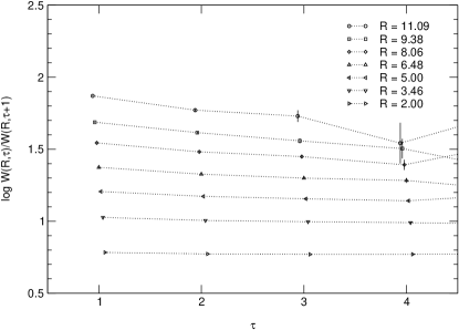
Figure 1: The effective potential, $V_{\mathrm{eff}}(R,\tau)$, at $(\beta,\kappa)=(5.32144,0.1665)$ on the $16^{3}$ lattice, for selected values of $R$ in the range $\tau=1,\dots,4$. Larger values of $\tau$ are dominated by statistical noise.

As can be seen from Fig. 2, the resulting values for $V(R)$ show the expected behavior.

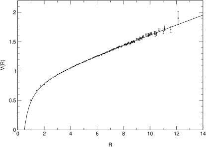
Figure 2: The static quark potential obtained from Wilson loops at $(\beta,\kappa)=(5.32144,0.1665)$ on the $16^{3}$ lattice.

We observe no indication of string breaking Bali et al. (2004) and therefore fit the data in the range $[R_{\mathrm{min}},R_{\mathrm{max}}]=[2.5,8]$ to

$$V(R)=V_{0}-\frac{e}{R}+\sigma R.$$ (22)

The upper boundary of the fit range was set to $R_{\mathrm{max}}=8$ because up to this value the data correspond nicely to the expected linear behavior, with small statistical errors. With $R_{\mathrm{max}}$ held fixed the lower boundary was determined by investigating the $R_{\mathrm{min}}$-dependence of $r_{0}$ for various values $R_{\mathrm{min}}\gtrsim 2$. (Below this value one observes a violation of rotational symmetry due to the finite lattice spacing.) From the fit we obtained the following parameters for the potential (in lattice units):

$$V_{0}=0.8378(87),\quad e=0.440(18),\quad\sigma=0.08187(97).$$

The Sommer scale $R_{0}$, which is defined through the force between two static quarks at some intermediate distance,

$$R^{2}\left.\frac{dV}{dR}\right|_{R=R_{0}}=1.65,$$ (23)

was obtained from these parameters according to

$$R_{0}=\sqrt{\frac{1.65-e}{\sigma}}.$$ (24)

Our result for the simulation at $(\beta,\kappa,L)=(5.32144,0.1665,16)$ is given in Table 4. The quoted uncertainty corresponds to the statistical error.

Table 4: Sommer scale and resulting momentum cut-off, lattice spacing and lattice size for $r_{0}=0.5$ fm.

$\beta$	$\kappa$	$L^{3}T$	$r_{0}/a$	$a^{-1}\,[\mathrm{GeV}]$	$a\,[\mathrm{fm}]$	$L\,[\mathrm{fm}]$
5.32144	0.1665	$16^{3}32$	3.845(37)	1.517(15)	0.1300(13)	2.081(21)
5.5	0.1580	$16^{3}32$	4.027(24)	1.5893(95)	0.12416(74)	1.987(12)
	0.1590	$16^{3}32$	4.386(26)	1.731(11)	0.11400(68)	1.824(11)
	0.1596	$16^{3}32$	4.675(34)	1.845(14)	0.10695(78)	1.711(13)
	0.1600	$16^{3}32$	4.889(30)	1.929(12)	0.10227(63)	1.636(10)
5.6	0.1560	$16^{3}32$	5.104(29)	2.014(12)	0.09796(56)	1.5674(89)
	0.1565	$16^{3}32$	5.283(52)	2.085(21)	0.09464(93)	1.514(15)
	0.1570	$16^{3}32$	5.475(72)	2.161(29)	0.0913(12)	1.461(20)
	0.1575	$16^{3}32$	5.959(77)	2.352(31)	0.0839(11)	1.343(18)
		$24^{3}40$	5.892(27)	2.325(11)	0.08486(39)	2.0367(94)
	0.1580	$24^{3}40$	6.230(60)	2.459(24)	0.08026(78)	1.926(19)

We used $r_{0}=0.5$ fm to set the scale in our simulations. The resulting physical values for the momentum cut-off $a^{-1}$, the lattice spacing $a$ and the box size $L$ are displayed in Table 4. The smallest simulated $\beta$ of 5.32144 is associated with a lattice spacing of $a=0.13$ fm, corresponding to a momentum cut-off of 1.52 GeV. While we have to watch out for potentially large $O(a)$ discretization errors at this coupling, the physical volume is the biggest of all simulated volumes. With a linear extension of slightly more than 2 fm it is comparable in size with the T$\chi$L lattice at $(\beta,\kappa)=(5.6,0.1575)$.

IV.2 Hadron masses and decay amplitudes

In order to extract meson masses and amplitudes we followed the standard procedure of computing zero-momentum 2-point functions ($x=(\mathbf{x},\tau)$)

$$\bigl{\langle}{\mathcal{O}^{\dagger}(\tau)\mathcal{O}(0)}\bigr{\rangle}\equiv\sum_{\mathbf{x}}\bigl{\langle}{\mathcal{O}^{\dagger}(x)\mathcal{O}(0)}\bigr{\rangle}$$ (25)

for the following pseudoscalar and vector operators:

$$P(x) =\overline{q}^{\prime}(x)\gamma_{5}q(x),$$ (26a)

$$A_{4}(x) =\overline{q}^{\prime}(x)\gamma_{5}\gamma_{4}q(x),$$ (26b)

$$V_{k}(x) =\overline{q}^{\prime}(x)\gamma_{k}q(x).$$ (26c)

For the nucleon we have used the octet baryon operator

$$N(x)=\epsilon_{abc}\bigl{(}q^{T}_{a}(x)C\gamma_{5}q^{\prime}_{b}(x)\bigr{)}q_{c}^{\prime\prime}(x),$$ (27)

where $a,b,c$ are color indices and $C=\gamma_{4}\gamma_{2}$ is the charge conjugation matrix. We employed the gauge invariant Wuppertal smearing Güsken (1990) at the source only ($ls$) or at both source and sink ($ss$). In the previous SESAM and T$\chi$L simulations $N=50$ smearing steps were used with a weight of $\alpha=4.0$. These parameters were originally optimized for the $16^{3}$ SESAM lattice and then adopted for the larger $24^{3}$ T$\chi$L lattice, too. In order to adapt these parameters to our smaller lattices we have investigated the effect of smearing on the various volumes. We applied the Wuppertal smearing procedure to point sources $\phi^{(0)}(\mathbf{x})$ of size $L^{3}$ with $L=24,16,14,12,10$. We set $\phi^{(0)}(\mathbf{x})\equiv 0$ except for the point at $(L/2,L/2,L/2)$, which we defined as the origin of the respective lattice and where we set $\phi^{(0)}(\mathbf{0})=1$. Applying the smearing prescription $N$ times to $\phi^{(0)}$ with all $U_{\mu}(\mathbf{x})\equiv 1$ we plot the amplitude of the resulting wave function $\phi^{(N)}$ along the (arbitrarily chosen) $(0,0,1)$-direction relative to its maximum at the origin, i.e. $\lvert{\phi^{(N)}(0,0,x_{3})}\rvert^{2}/\lvert{\phi^{(N)}(\mathbf{0})}\rvert^{2}$, versus $x_{3}/L$, for various values of $N$ and $\alpha$. On inspection of the resulting wave function shapes we selected the parameters $N$ and $\alpha$ for our simulated volumes so as to make the respective wave function profile look approximately like the SESAM one. The chosen smearing parameters are listed in Table 5, while the corresponding wave function profiles are displayed in Fig. 3.

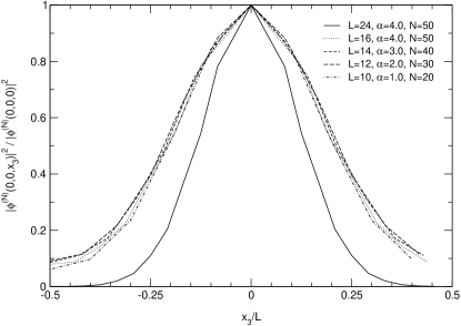
Figure 3: The parameters $N$, $\alpha$ for the Wuppertal smearing scheme were chosen such as to yield approximately the same wave function shapes for both the smaller lattices and the SESAM lattice ($L=16$).

Table 5: Smearing parameters.

$L$	10	12	14	16	24
$\alpha$	1.0	2.0	3.0	4.0	4.0
$N$	20	30	40	50	50

The masses and amplitudes of mesons were obtained by correlated least-$\chi^{2}$ fits of the (time-symmetrized) correlators $\bigl{\langle}{\mathcal{O}^{\dagger}(\tau)\mathcal{O}(0)}\bigr{\rangle}$, $\mathcal{O}=P,A_{4},V_{k}$, to the parameterization

$$f^{M}_{\tau}(C,M)=C\left(e^{-M\tau}+e^{-M(T-\tau)}\right),$$ (28)

where $M\equiv am$ is the mass and $C\sim|\langle{0}\left|{\mathcal{O}}\right|{p}\rangle|^{2}/2M$ if $|\textstyle{p}\rangle$ is the zero-momentum state of the particle associated with $\mathcal{O}$. In the case of the nucleon we fitted the correlator (anti-symmetrized in $\tau$ and $T-\tau$) to the single exponential

$$f^{B}_{\tau}(C,M)=Ce^{-M\tau}.$$ (29)

The optimal lower limits of the fit intervals, $\tau_{\mathrm{min}}$, were found as usual by examining the $\chi^{2}/\mathrm{dof}$-behavior and the stability of the masses with respect to $\tau_{\mathrm{min}}$, and by inspection of the effective masses. The upper limit, $\tau_{\mathrm{max}}$, was in general kept fixed at $T/2$ for mesons and $T/2-1$ for the nucleon.

Table 6: Masses of the pseudoscalar and vector mesons and of the nucleon, the pseudoscalar decay constant and the PCAC quark mass in lattice units.

$\beta$	$\kappa$	$L^{3}T$	$m_{\mathrm{PS}}L$	$M_{\mathrm{PS}}$	$M_{\mathrm{V}}$	$M_{N}$	$Z_{A}^{-1}F_{\mathrm{PS}}$	$Z_{q}M_{q}$
5.32144	0.1665	$12^{3}32$	3.18(8)	0.2648(67)	0.508(26)	0.788(26)	0.062(10)	0.0106(33)
		$14^{3}32$	3.6(1)	0.2577(87)	0.518(12)	0.779(16)	0.0757(56)	0.0152(18)
		$16^{3}32$	4.42(7)	0.2760(42)	0.4999(78)	0.727(11)	0.0843(62)	0.0155(12)
5.5	0.1580	$16^{3}32$	8.85(6)	0.5534(39)	0.6506(46)	1.026(18)	0.1073(42)	0.0821(35)
	0.1590	$16^{3}32$	7.09(4)	0.4429(26)	0.5529(54)	0.8718(78)	0.0945(23)	0.0544(12)
	0.1596	$16^{3}32$	5.89(4)	0.3682(27)	0.4902(52)	0.7640(75)	0.0815(16)	0.03724(81)
	0.1600	$16^{3}32$	4.89(5)	0.3058(34)	0.4547(61)	0.703(10)	0.0750(23)	0.0279(15)
5.6	0.1560	$16^{3}32$	7.15(4)	0.4469(23)	0.5365(36)	0.8533(62)	0.0843(19)	0.0620(11)
	0.1565	$16^{3}32$	6.32(6)	0.3948(38)	0.4989(54)	0.785(10)	0.0805(18)	0.0467(15)
	0.1570	$16^{3}32$	5.52(5)	0.3452(29)	0.4527(52)	0.7095(90)	0.0726(16)	0.0391(15)
	0.1575	$10^{3}32$	4.92(6)	0.4919(55)	0.587(20)	1.042(20)	0.0284(30)	0.0209(32)
		$12^{3}32$	4.3(1)	0.3576(89)	0.494(12)	0.817(16)	0.0429(34)	0.0249(19)
		$14^{3}32$	4.27(6)	0.3048(44)	0.4413(66)	0.719(16)	0.0566(30)	0.0261(22)
		$16^{3}32$	4.49(6)	0.2806(35)	0.4036(68)	0.6254(89)	0.0626(26)	0.0275(16)
		$24^{3}40$	6.64(6)	0.2765(26)	0.3944(38)	0.5920(75)	0.0646(18)	0.02680(68)
	0.1580	$12^{3}32$	4.6(1)	0.387(12)	0.535(17)	0.882(25)	0.022(12)	0.0113(88)
		$14^{3}32$	4.13(8)	0.2949(60)	0.4677(90)	0.717(19)	0.0233(32)	0.0099(17)
		$16^{3}32$	3.72(8)	0.2325(51)	0.371(13)	0.622(12)	0.0469(26)	0.0141(11)
		$24^{3}40$	4.78(8)	0.1991(33)	0.3519(86)	0.500(12)	0.0602(39)	0.0157(11)

Table 7: Masses of the pseudoscalar meson, the vector meson and the nucleon in physical units (using $r_{0}=0.5$ fm).

$\beta$	$\kappa$	$L^{3}T$	$L\,[\mathrm{fm}]$	$(r_{0}m_{\mathrm{PS}})^{2}$	$m_{\mathrm{PS}}/m_{\mathrm{V}}$	$m_{\mathrm{PS}}\,[\mathrm{GeV}]$	$m_{\mathrm{V}}\,[\mathrm{GeV}]$	$m_{N}\,[\mathrm{GeV}]$
5.32144	0.1665	$12^{3}32$	1.56(2)	1.037(57)	0.521(23)	0.402(11)	0.771(40)	1.195(42)
		$14^{3}32$	1.82(2)	0.982(68)	0.497(20)	0.391(14)	0.786(20)	1.182(26)
		$16^{3}32$	2.08(2)	1.126(43)	0.552(11)	0.4188(75)	0.759(14)	1.104(20)
5.5	0.1580	$16^{3}32$	1.99(1)	4.97(20)	0.8506(31)	0.8795(81)	1.0340(95)	1.631(30)
	0.1590	$16^{3}32$	1.82(1)	3.77(12)	0.8010(53)	0.7666(64)	0.957(11)	1.509(16)
	0.1596	$16^{3}32$	1.71(1)	2.96(10)	0.7512(51)	0.6793(70)	0.904(12)	1.410(17)
	0.1600	$16^{3}32$	1.64(1)	2.235(85)	0.6725(93)	0.5901(75)	0.877(13)	1.356(21)
5.6	0.1560	$16^{3}32$	1.567(9)	5.20(18)	0.8330(16)	0.9002(69)	1.0807(94)	1.719(16)
	0.1565	$16^{3}32$	1.51(1)	4.35(25)	0.7912(72)	0.823(11)	1.040(15)	1.637(27)
	0.1570	$16^{3}32$	1.46(2)	3.57(21)	0.7627(58)	0.746(12)	0.978(17)	1.533(28)
	0.1575	$10^{3}32$	0.849(4)	8.40(59)	0.838(30)	1.144(14)	1.365(48)	2.424(47)
		$12^{3}32$	1.018(5)	4.44(48)	0.724(11)	0.832(21)	1.149(27)	1.901(38)
		$14^{3}32$	1.188(5)	3.22(18)	0.691(11)	0.709(11)	1.026(16)	1.671(39)
		$16^{3}32$	1.358(6)	2.73(12)	0.6952(99)	0.6524(86)	0.938(16)	1.454(22)
		$24^{3}40$	2.037(9)	2.654(90)	0.7010(62)	0.6429(67)	0.9171(98)	1.377(19)
	0.1580	$12^{3}32$	0.963(9)	5.80(88)	0.722(20)	0.951(30)	1.316(44)	2.167(66)
		$14^{3}32$	1.12(1)	3.37(28)	0.630(13)	0.725(16)	1.150(25)	1.763(50)
		$16^{3}32$	1.28(1)	2.10(15)	0.627(21)	0.572(14)	0.912(33)	1.530(32)
		$24^{3}40$	1.93(2)	1.539(74)	0.566(17)	0.4896(94)	0.865(23)	1.228(31)

The masses (in lattice units) of the pseudoscalar and vector mesons and of the nucleon are listed in Table 6. As the masses from the $ls$ and the $ss$ correlators are consistent we only quote the values extracted from the latter. The quoted errors are statistical in nature and have been estimated with the jackknife method (after suitable blocking of the data). Table 6 also shows $m_{\mathrm{PS}}(L)L$, the linear box size in units of the pseudoscalar correlation length $1/m_{\mathrm{PS}}(L)$, where $m_{\mathrm{PS}}(L)$ is the pion mass in the given finite volume. It should be borne in mind that for sub-asymptotic volumes this value is in general significantly different from $m_{\mathrm{PS}}L$, where $m_{\mathrm{PS}}$ is the pseudoscalar mass in infinite volume. At $(\beta,\kappa)=(5.32144,0.1665)$ we attain our lightest quark mass, with $m_{\mathrm{PS}}/m_{\mathrm{V}}$ being close to 0.5. Using $r_{0}=0.5$ fm to set the physical scale the hadron masses of Table 6 translate into the values listed in Table 7. This table shows also the physical box sizes $L\,[\mathrm{fm}]$ which have been calculated using the lattice spacing $a$ from the largest available lattice, respectively (see also Table 4). The dimensionless quantity

$$M_{r}=(r_{0}m_{\mathrm{PS}})^{2}$$ (30)

is another measure of the quark mass, since for $m_{q}\to 0$ the pion mass behaves like $m_{\pi}\propto\sqrt{m_{q}}$. At the physical strange quark mass it gives $M_{r}\approx 3.1$ Farchioni et al. (2002). At those parameter sets where we have simulated several lattice volumes the value of $M_{r}$ ranges between $M_{r}\approx 2.65$ and $M_{r}\approx 1.13$, corresponding to about 85 and 36% of the value for the strange quark mass.

The (unrenormalized) pseudoscalar decay constant, which is defined on the lattice by (for $\mathbf{p}=\mathbf{0}$)

$$Z_{A}\,\langle{0}\left|{A_{4}}\right|{\mathrm{PS}}\rangle=M_{\mathrm{PS}}F_{\mathrm{PS}},$$ (31)

has been obtained from

$$Z_{A}^{-1}F_{\mathrm{PS}}=\sqrt{\frac{2C_{A}^{ll}}{M_{\mathrm{PS}}}}=C_{A}^{ls}\sqrt{\frac{2}{M_{\mathrm{PS}}C_{A}^{ss}}},$$ (32)

where we have used the fact that amplitudes for local source and sink ($ll$) can be obtained from $ls$ and $ss$ amplitudes according to

$$C^{ll}=\frac{(C^{ls})^{2}}{C^{ss}}.$$ (33)

The pseudoscalar mass $M_{\mathrm{PS}}=M_{P}^{ss}$ in Eq. (32) has been taken from a fit of $\bigl{\langle}{P^{\dagger}(\tau)P(0)}\bigr{\rangle}^{ss}$, the amplitudes $C_{A}^{ls}$ ($C_{A}^{ss}$) from a fit of the local-smeared (smeared-smeared) correlator $\bigl{\langle}{A_{4}^{\dagger}(\tau)A_{4}(0)}\bigr{\rangle}^{ls(ss)}$.

In order to determine the (unrenormalized) quark mass $M_{q}\equiv am_{q}$ as defined via the PCAC relation on the lattice,

$$M_{q}=-\frac{M_{\mathrm{PS}}}{2}\frac{Z_{A}}{Z_{P}}\frac{\langle{0}\left|{A_{4}}\right|{\mathrm{PS}}\rangle}{\langle{0}\left|{P}\right|{\mathrm{PS}}\rangle},$$ (34)

we used the relation

$$Z_{q}M_{q}=\frac{M_{\mathrm{PS}}}{2}\sqrt{\frac{C_{A}^{ll}}{C_{P}^{ll}}}=\frac{M_{\mathrm{PS}}}{2}\frac{C_{A}^{ls}}{C_{P}^{ls}}\sqrt{\frac{C_{P}^{ss}}{C_{A}^{ss}}},$$ (35)

where the renormalization constant is defined as $Z_{q}\equiv Z_{P}/Z_{A}$ and the pseudoscalar mass is taken to be the average

$$M_{\mathrm{PS}}=\frac{1}{4}\left(M_{P}^{ls}+M_{P}^{ss}+M_{A}^{ls}+M_{A}^{ss}\right).$$ (36)

Our results (in lattice units) for the unrenormalized pseudoscalar decay constant $F_{\mathrm{PS}}/Z_{A}$ are displayed in Table 6. The normalization of the pseudoscalar decay constant is such that the physical value is $f_{\pi}=92.4$ MeV. The same table also shows the results for the bare PCAC quark mass $Z_{q}M_{q}$.

V Volume dependence of pion and nucleon masses

The three parameter sets at which we have data from several lattice volumes, namely $(\beta,\kappa)=(5.6,0.1575)$, $(5.6,0.158)$ and $(5.32144,0.1665)$, are characterized by the quark mass, which in turn can be expressed in terms of the pion mass via the GMOR relation. We quote the pion mass measured on the largest lattice, respectively, when we refer to a particular simulation point $(\beta,\kappa)$. We have investigated the volume dependence of the pion, the rho and the nucleon at pion masses (before continuum extrapolation) of approximately 643 MeV, 490 MeV and 419 MeV in the ranges 0.85–2.04 fm, 0.96–1.93 fm and 1.56–2.08 fm, respectively. Due to angular momentum conservation the decay $\rho\to\pi\pi$ is suppressed on small lattices where the minimum non-zero momentum $2\pi/L$ is large. We therefore incorporate the rho resonance in our phenomenological analysis of finite-size effects, because on the lattices considered here it should be stable.

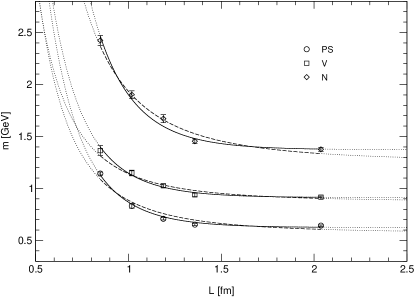
Figure 4: Box-size dependence of the pseudoscalar and vector meson masses and of the nucleon mass at $(\beta,\kappa)=(5.6,0.1575)$. The solid lines result from fits to an exponential, Eq. (38), while the dashed lines represent fits to a power law, Eq. (39). The curves are dotted outside the fit interval.

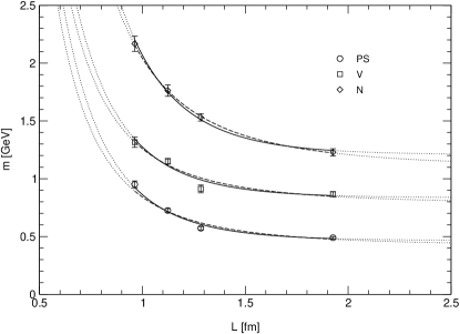
Figure 5: Fits as in Fig. 4 for $(\beta,\kappa)=(5.6,0.158)$.

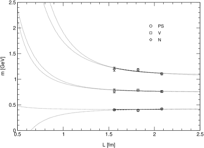
Figure 6: Fits as in Fig. 4 for $(\beta,\kappa)=(5.32144,0.1665)$. The fact that the pion and the rho show no monotonous increase of the finite-size shift towards decreasing box-size is ascribed to the smallness of the effect and statistics. (The simulations of the smaller lattices in particular at $\beta=5.32144$ were affected by sizeable fluctuations.) In the case of the nucleon the finite-size effect is somewhat more significant.

Table 8: Ratios of the pseudoscalar mass and the chiral symmetry breaking scale, and the relative finite-size effects according to Eq. (37).

$\beta$	$\kappa$	$L^{3}T$	$\displaystyle\frac{M_{\mathrm{PS}}}{4\pi Z_{A}^{-1}F_{\mathrm{PS}}}$	$R_{\mathrm{PS}}$	$R_{\mathrm{V}}$	$R_{N}$
5.32144	0.1665	$12^{3}32$	$0.34(6)$	-0.04(3)	0.02(5)	0.08(4)
		$14^{3}32$	$0.27(2)$	-0.07(3)	0.04(3)	0.07(3)
		$16^{3}32$	$0.26(2)$	0	0	0
5.6	0.1575	$10^{3}32$	$1.4(1)$	0.78(3)	0.49(5)	0.76(4)
		$12^{3}32$	$0.66(6)$	0.29(3)	0.25(3)	0.38(3)
		$14^{3}32$	$0.43(2)$	0.10(2)	0.12(2)	0.21(3)
		$16^{3}32$	$0.36(2)$	0.01(2)	0.02(2)	0.06(2)
		$24^{3}40$	$0.341(10)$	0	0	0
	0.1580	$12^{3}32$	$1.4(8)$	0.94(7)	0.52(6)	0.76(7)
		$14^{3}32$	$1.0(1)$	0.48(4)	0.33(4)	0.44(5)
		$16^{3}32$	$0.39(2)$	0.17(3)	0.05(5)	0.25(4)
		$24^{3}40$	$0.26(2)$	0	0	0

Figs. 4–6 show, for our three different quark masses, the pion, rho and nucleon masses in physical units as functions of the box-size. In Table 8 we list the relative differences of the masses measured at $L$ and $L_{\mathrm{max}}$,

$$R_{H}(L)=\frac{M_{H}(L)-M_{H}(L_{\mathrm{max}})}{M_{H}(L_{\mathrm{max}})},$$ (37)

where $H=\mathrm{PS},\mathrm{V},\mathrm{N}$ and $L_{\mathrm{max}}=24$ ($L_{\mathrm{max}}=16$) for $\beta=5.6$ ($\beta=5.32144$). For both quark masses at $\beta=5.6$ we find a large variation of the hadron masses over the considered range of lattice sizes. While the finite-size effects in the pion, rho and nucleon masses are relatively small (of the order of a few percent) if one compares only the two largest lattices at $\kappa=0.1575$, they rapidly grow on the smaller volumes ($\sim 50$–$80\%$ at $L=10$). The rate of the increase is hadron dependent: while at large $L$ the pion has the smallest relative finite-size effect, the relative shift in the pion mass grows strongest with decreasing $L$, until it exceeds the effect in the rho mass from $L=12$ and that in the nucleon mass from $L=10$ downwards. Considering the finite-size effects at $\kappa=0.158$ (corresponding to a lower quark mass) we notice that at a given value of $L$ the finite-size effects are generally much larger at $\kappa=0.158$ than at $0.1575$. Again we observe that the pion is subject to the strongest relative effect in the regime of small volumes. Finally, at $(\beta,\kappa)=(5.32144,0.1665)$ (corresponding to the lightest of our quark masses), we find rather small finite-size effects of only a few percent in the simulated $L$-range, for all considered hadrons. In view of the small $m_{\mathrm{PS}}L$ values (see Table 7) this is quite remarkable: if the finite-size effects would only depend on $m_{\mathrm{PS}}L$ we would expect the effects at $\beta=5.32144$ to be of about the same order of magnitude as those at the smaller volumes at $\beta=5.6$. On the other hand, due to the large lattice spacing the volumes at $\beta=5.32144$ are, in terms of the physical size, comparable with the larger volumes at $\beta=5.6$. This strongly suggests that there are, in fact, different mechanisms responsible for the observed mass shifts, and that the transition between them is in our case characterized by the absolute physical lattice size rather than the product $m_{\mathrm{PS}}L$. Quite independently of the pion mass the region in $L$ where finite-size shifts start to become large is located at around 1.5 fm in our simulations.

V.1 Fits of the volume dependence

First we attempted to describe the volume dependence of our simulated masses phenomenologically by fitting them to two different parameterizations. One of these parameterizations is inspired by Lüscher’s exponential leading-order mass shift formula (5) for the pion, while the other one is directly given by the power law observed by Fukugita et al., Eq. (10). Although neither of these approaches can a priori be expected to be valid over the entire range of considered lattice volumes, and although Lüscher’s formula strictly speaking has no free fit parameters, on practical grounds it is still interesting whether based on either of the two functional forms an empirical description can be found that connects small and medium-sized volumes to the asymptotic regime.

The curves in Figs. 4 and 5 show fits of the data for the pion, rho and nucleon masses ($H=\text{PS,V,N}$) to the exponential function

$$m_{H}(L)=m_{H}+cL^{-\frac{3}{2}}e^{-m_{\mathrm{PS}}L},$$ (38)

and, for comparison, to the power law

$$m_{H}(L)=m_{H}+cL^{-3}.$$ (39)

In the case of the pion (where $m_{H}=m_{\mathrm{PS}}$) the mass $m_{\mathrm{PS}}$ in Eq. (38) was treated as a fit parameter; the result was used as input for the fits of the rho and the nucleon data, so that all the fits displayed in Figs. 4 and 5 had two free parameters. As can be seen from the plots both parameterizations describe the data reasonably well within the fit interval, but regarding the asymptotic behavior the exponential ansatz is clearly superior. At $(\beta,\kappa)=(5.6,0.1575)$, for example, all infinite-volume masses $m_{H}$ resulting from the exponential fits are compatible with the data from the largest, $24^{3}$ lattice, which are assumed to bear no significant finite-size effects. In contrast, fitting the data to the power law yields numbers for $m_{H}$ that grossly underestimate the true asymptotic masses. Varying the right boundary of the fit interval we find that for small box-sizes ($L\lesssim 1.5$ fm) where the finite-size effects are of the order of several percent the power law provides an acceptable description of the data. At the two larger quark masses this corresponds to the regime of $m_{\mathrm{PS}}L\lesssim 4.5..4.8$, in accordance with the common rule of thumb that only for $m_{\mathrm{PS}}L\gtrsim 5$ finite-size mass shifts are exponentially suppressed. (In the light of our results at $(\beta,\kappa)=(5.32144,0.1665)$ it appears as if this rule of thumb could be relaxed as long as as the physical lattice extent $L$ remains sufficiently large.) We find that as soon as we include data from larger volumes (where the mass shifts are small) into the fits the exponential ansatz yields better values for both $\chi^{2}/\mathrm{dof}$ and $m_{H}$. In order to test whether this ansatz is suitable for an extrapolation from the small lattices to the infinite volume we fitted the masses at $(\beta,\kappa)=(5.6,0.1575)$ and $(5.6,0.158)$ only up to $L=16$. Assuming that the finite-size effects on the $24^{3}$ lattice are not significant it can be seen from Figs. 7 and 8 that the asymptotic pion masses are generally underestimated considerably, while in the case of the nucleon mass the extrapolation works rather well. In either case the the extrapolation tends to yield lower bounds to the infinite-volume masses, the systematic uncertainty of which can be estimated by varying the boundaries of the fit intervals.

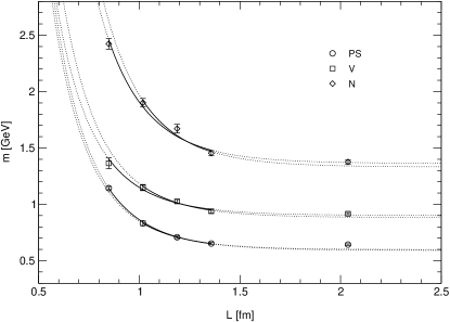
Figure 7: Infinite-volume extrapolation of the masses at $(\beta,\kappa)=(5.6,0.1575)$. The solid lines correspond to exponential fits according to Eq. (38). The curves are dotted outside the fit intervals.

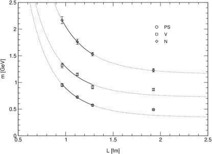
Figure 8: Extrapolations as in Fig. 7 for $(\beta,\kappa)=(5.6,0.158)$.

It should be mentioned that alternative fit formulae (obtained e.g. by changing the exponent of $L$ from $-3/2$ to $-1$ in Eq. (38), introducing an additional variable factor in the exponential of Eq. (38), or treating the exponent of $L$ as a free parameter in Eq. (39)) may also be used to describe the data. They do not, however, lead to significant improvements and/or require even more free parameters.

The main lesson we have learned from this exercise is the following: If one has got hadron masses from more than two different lattice volumes (at fixed coupling and quark mass) and wants to estimate the infinite-volume masses on the basis of a fit, one should use an exponential ansatz rather than the power law. Extrapolating the exponential fit will produce lower bounds to the true asymptotic masses, and these bounds are generally better than those that can be obtained with the power law.

V.2 Applicability of Chiral Perturbation Theory

In order to better understand why it is problematic to extrapolate from small volumes to the infinite volume on the basis of the simple formulae (38) and (39) one needs to appreciate their respective origin and scope. The power law (39) is supposed to originate from a distortion of the hadron wave function (or from a modification of the effect of virtual particles traveling around the lattice by a model-dependent form factor that accounts for the finite hadron extent Fukugita et al. (1992b)) at quite small volumes. Consequently, the $L^{-3}$-behavior is not expected to persist towards large volumes, which is in fact borne out by our data. On the other hand, the formula (38) essentially corresponds to Lüscher’s asymptotic formulae for the pion. Lüscher’s general formula for the volume dependence of stable particles in a finite volume represents the leading term of a large $L$ expansion, meaning that whenever the relative suppression factor

$$\frac{\text{subleading}}{\text{leading}}=O\left(e^{-(\bar{m}-m_{\pi})L}\right)$$ (40)

is not small, subleading effects may be of practical relevance.

V.2.1 Pion

In the case of the pion we also rely on effective field theory to provide us with an analytic expression for the elastic forward scattering amplitude $F_{\pi\pi}$. At leading order in the chiral expansion this amplitude is given by the constant expression $F_{\pi\pi}=-m_{\pi}^{2}/f_{\pi}^{2}$. Inserting this into the Lüscher formula eventually leads to Eq. (5), which has the functional form of our exponential ansatz (38). We have seen that the data can be described quite well by the parameterization (38). It is therefore instructive to compare our results for the parameter $c$ to the constant

$$C=\frac{3}{4(2\pi)^{3/2}}\frac{m_{\mathrm{PS}}^{3/2}}{(Z_{A}^{-1}f_{\mathrm{PS}})^{2}}$$ (41)

(cf. Eq. (5)), where at each $(\beta,\kappa)$ we take $m_{\mathrm{PS}}$ and $Z_{A}^{-1}F_{\mathrm{PS}}$ from the largest available lattice, respectively (see Table 6). For our simulation points $(\beta,\kappa)=(5.6,0.1575)$, $(5.6,0.158)$ and $(5.32144,0.1665)$ we have $C/\mathrm{GeV}^{-1/2}=1.089(61)$, $0.745(98)$ and $0.79(12)$, respectively. (Using $m_{\pi}=137$ MeV and $f_{\pi}=92.4$ MeV the natural value is $C=0.283\,\mathrm{GeV}^{-1/2}$.) Comparing the first two of these values to the results for $c$ in Tables 13 and 13 (exp,PS) we see that the relative factor between $c$ and $C$ is $O(10)$ assuming that $Z_{A}=O(1)$. The discrepancy is generally larger for smaller values of the left fit boundary, $L_{1}$, but decreases for increasing $L_{1}$.

The large differences between the coefficients $c$ from the fits to our pion data and $C$ from the Lüscher formula (with LO ChPT input) reflect the fact that not all of our data sets for the different volumes at $(\beta,\kappa)=(5.6,0.1575)$ and $(5.6,0.158)$ comply with the conditions under which the application of this formula is justified. Recall that these conditions are: (i) sufficiently large lattice volumes (because the Lüscher formula corresponds to the leading term in a large $L$ expansion), and (ii) small pion masses (because we take the pion scattering amplitude from chiral perturbation theory).

Quite recently, the finite-size shift of the pion mass has been determined using Lüscher’s formula with the $\pi\pi$ forward scattering amplitude taken from two-flavor chiral perturbation theory up to NNLO in the chiral expansion Colangelo and Dürr (2004). These results have then been compared to the leading order chiral expression for the pion mass in finite volume (including the large-$L$ suppressed terms neglected by the Lüscher formula) in order to estimate the effect of subleading terms in the large $L$ expansion. Both aspects of this investigation rely on chiral perturbation theory as an expansion in the pion mass $m_{\pi}$ and the particle momenta $p$, both of which have to be small compared to the chiral symmetry breaking scale that is usually identified with $4\pi f_{\pi}$. The conditions of applicability thus read

$$\frac{m_{\pi}}{4\pi f_{\pi}}\ll 1$$ (42)

and

$$\frac{p}{4\pi f_{\pi}}\ll 1.$$ (43)

In a periodic finite box of size $L$, where the particles’ momenta can only take discrete values $p_{k}=2\pi n_{k}/L$ with $n_{k}\in\mathbb{Z}$, the second condition directly translates into a bound on the box size,

$$L\gg\frac{1}{2f_{\pi}}\sim 1\mathrm{fm},$$ (44)

where we have used the physical value of $f_{\pi}$. (As shown in Ref. Colangelo and Dürr (2004) the pion mass dependence of $f_{\pi}$ predicted by ChPT at NNLO is rather mild.) While a priori it is not clear what the practical significance of the relations (42) and (44) is, we can identify on the basis of Tables 8 and 7 those data sets that stand the greatest chance of meeting these conditions. From Table 8 one can see that the ratios $M_{\mathrm{PS}}(L)/(4\pi Z_{A}^{-1}F_{\mathrm{PS}}(L))$ for all simulated volumes at $(\beta,\kappa)=(5.32144,0.1665)$ are relatively small and compatible with each other. The corresponding ratio at $(\beta,\kappa)=(5.6,0.158)$ is also relatively small for $L=L_{\mathrm{max}}$ (and, moreover, comparable to the numbers at $(5.32144,0.1665)$), but the value for the second largest lattice is already significantly larger. Considering only the largest lattice, respectively, $M_{\mathrm{PS}}/(4\pi Z_{A}^{-1}F_{\mathrm{PS}})$ is largest at $(\beta,\kappa)=(5.6,0.1575)$, but here the value at $L=16$ is still consistent with the one at $L_{\mathrm{max}}=24$. In view of this and recalling the relative finite-size mass shifts $R$ (Table 8) we infer from Table 7 that for $m_{\pi}=643$ MeV and $m_{\pi}=490$ MeV we can trust ChPT at most on the largest volumes with $L\approx 2$ fm (and possibly the $16^{3}$ lattice with $L\approx 1.4$ fm at $m_{\pi}=643$ MeV), while the lattices with $L<1.4$ fm are most probably too small. At $(\beta,\kappa)=(5.32144,0.1665)$, on the other hand, where $m_{\pi}=419$ MeV, all lattices are larger than 1.5 fm due to the relatively large lattice spacing, and hence appear large enough for ChPT to be applicable.

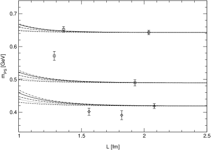
Figure 9: Volume dependence of our pion masses in the regime $L\gtrsim 1.3$ fm. The circles, squares and diamonds represent our data at $(\beta,\kappa)=(5.6,0.1575)$ ($m_{\pi}=643$ MeV), $(\beta,\kappa)=(5.6,0.158)$ ($m_{\pi}=490$ MeV) and $(\beta,\kappa)=(5.32144,0.1665)$ ($m_{\pi}=419$ MeV), respectively. The curves correspond to Lüscher’s formula with input from ChPT at LO (dashed), NLO (long-dashed) and NNLO (solid). The dotted curves show the full LO chiral expression. The dash-dotted curve is the full LO result shifted by the difference between the NNLO and the LO Lüscher formula.

In order to corroborate these findings we checked how our simulated pion masses $m_{\mathrm{PS}}(L)$, for $L\gtrsim 1.3$ fm, relate to the results of Ref. Colangelo and Dürr (2004). There, the chiral expression for the amplitude $F_{\pi\pi}$ has been written as an expansion in powers of $\xi$,

$$F_{\pi\pi}=16\pi^{2}\left[\xi F_{2}+\xi^{2}F_{4}+\xi^{3}F_{6}+O(\xi^{4})\right],$$ (45)

where the parameter $\xi$ is defined as

$$\xi=\left(\frac{m_{\pi}}{4\pi f_{\pi}}\right)^{2}.$$ (46)

Inserting the expansion (45) up to $F_{4}$ or $F_{6}$ into Lüscher’s formula (3) for the pion and using the chiral expression for the isospin invariant amplitude $A$ of Ref. Bijnens et al. (1996), the leading term in the large-$L$ expansion is obtained up to NLO and NNLO in the chiral expansion. (Correspondingly, inserting (45) into (3) only up to $F_{2}$ yields the LO expression (4).) In order to calculate the predicted finite size shift for the pion numerically for our three different pion masses we need to know the respective numerical value of the expansion parameter $\xi$. In order to avoid the difficulties associated with the renormalization of the pion decay constant one can use the analytic expression for the pion mass dependence of $f_{\pi}$ which is known to NNLO in ChPT. If we take the pion mass from the largest lattice as a first approximation to the asymptotic pion mass $m_{\pi}$, respectively, we obtain the curves displayed in Fig. 9. The dashed curves correspond to Lüscher’s formula (4) with $F_{\pi\pi}$ from ChPT at leading order. The long-dashed and solid curves show the NLO and NNLO predictions, respectively. For comparison, the dotted curves show the full leading-order chiral expression ($N_{f}=2$) for the pion mass in finite volume, given by

$$m_{\pi}(L)=m_{\pi}\left[1+\xi\sum_{n=1}^{\infty}\,m(n)\,\frac{K_{1}(\sqrt{n}\,m_{\pi}L)}{\sqrt{n}\,m_{\pi}L}\right],$$ (47)

where the multiplicity $m(n)$ counts the number of integer vectors $\mathbf{n}$ satisfying $n_{1}^{2}+n_{2}^{2}+n_{3}^{2}=n$ Colangelo and Dürr (2004). Since the modified Bessel function $K_{1}(x)$ falls off exponentially for large $x$, the sum in (47) is rapidly converging. For $n=1$ Eq. (47) corresponds precisely to the LO Lüscher formula (4). Finally, the dash-dotted curve in Fig. 9 represents the best currently available estimate of the full finite-size effect, obtained by adding to the Lüscher formula with $F_{\pi\pi}$ at NNLO the difference between Eq. (47) and the Lüscher formula with $F_{\pi\pi}$ at LO.

The main conclusion we draw from the plot is that for all our three pion masses and for our lattices with $L\gtrsim 1.3$ fm the finite-size effects predicted by ChPT are considerably smaller than our statistical errors. On the largest lattices with $L\simeq 2$ fm the maximal predicted finite-size correction (corresponding to the dash-dotted curve in the plot) is about 0.3% for the lightest pion and 0.05% for the heaviest one. This is in accordance with our presumption that for all practical purposes the finite-size effects in the pion masses are negligible on our largest lattices. At $L\simeq 1.3$ fm the finite-size shift ranges between 1% for the heaviest and about 3% for the lightest pion, which is of the order of the statistical uncertainties. For $L\gtrsim 1.3$ fm the differences between the full one-loop ChPT result and Lüscher’s formula with $F_{\pi\pi}$ at LO are comparably small, indicating that here the use of Lüscher’s asymptotic formula is indeed justified; the maximal difference in the relative effects is about 50% at $L\simeq 1.3$ fm for the smallest pion mass. By contrast, the difference between the relative effects predicted by Lüscher’s formula with $F_{\pi\pi}$ at NNLO and LO amounts, for the same lattice size, to a factor of 3.2 for the lightest and 4.5 for the heaviest pion.

Incidentally, a formula analogous to (47) exists also for the pion decay constant. (Recently also an asymptotic formula à la Lüscher has been derived for $f_{\pi}$ Colangelo and Haefeli (2004).) The only difference is that the relative finite size effect is negative and (for $N_{f}=2$) four times larger than that of the pion mass:

$$f_{\pi}(L)=f_{\pi}\left[1-4\xi\sum_{n=1}^{\infty}\,m(n)\,\frac{K_{1}(\sqrt{n}\,m_{\pi}L)}{\sqrt{n}\,m_{\pi}L}\right].$$ (48)

We have already seen that the volume dependence of our pion masses can be accounted for by chiral perturbation theory on the largest lattices at most, and there is no reason to believe that this should be different for the decay constant. But we can at least check whether we can recover the relative factor of minus four. Without going into the details we just state here that while we find the finite-size effect of the pion decay constant indeed to be negative, its magnitude is, on the smaller lattices at $(\beta,\kappa)=(5.6,0.1575)$ and $(5.6,0.158)$, about the same as that of the pion mass shift; on the second largest volume at $(\beta,\kappa)=(5.6,0.1575)$ the relative shift in $f_{\pi}(L)$ is about twice as big as the shift in $m_{\pi}(L)$. Unfortunately at $(\beta,\kappa)=(5.32144,0.1665)$, corresponding to our smallest quark mass, we can make no definite statement.

V.2.2 Nucleon

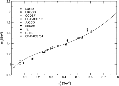
Figure 10: Nucleon mass data from various collaborations as a function of $m_{\pi}^{2}\propto m_{q}$, including our data. The curve corresponds to a fit of the data represented by the open symbols to Eq. (9). These data points are from simulations on relatively large and fine lattices. Note that the fit result is consistent with the physical pion and nucleon masses (indicated by the star).

Regarding the nucleon mass, replacing the simple exponential (38) by an ansatz corresponding more closely to Lüscher’s nucleon mass shift formula of Ref. Lüscher (1983) might be considered as the natural next step towards a better description of the volume dependence. (Although, as we have seen, the ansatz (38) describes the data already quite well.) But since Lüscher’s nucleon formula can be seen as a special case of the formula (7), let us instead confront our data for the nucleon mass directly with the formulae (II) and (7). Following Ref. Ali Khan et al. (2004) we fix $g_{A}$ and $f_{\pi}$ to the physical values $g_{A}=1.267$, $f_{\pi}=92.4$ MeV, and set the couplings $c_{2}$ and $c_{3}$ to $c_{2}=3.2\,\mathrm{GeV}^{-1}$, $c_{3}=-3.4\,\mathrm{GeV}^{-1}$. The remaining parameters $m_{0}$, $c_{1}$ and $e_{1}^{r}(\lambda)$ (where the renormalization scale $\lambda$ is chosen to be 1 GeV) are taken from a fit of data from various unquenched simulations with

$$a<\text{0.15~{}fm},\quad m_{\pi}L>5\quad\text{and}\quad m_{\pi}<\text{800~{}MeV}$$ (49)

to Eq. (9). In Ref. Ali Khan et al. (2004), data from the QCDSF Ali Khan et al. (2004), UKQCD Allton et al. (2002), CP-PACS Ali Khan et al. (2002) and JLQCD Aoki et al. (2003) collaborations have been used. These data are plotted in Fig. 10 (open symbols), complemented by the results from our largest lattices, namely the T$\chi$L results at $(\beta,\kappa,L)=(5.6,0.1575,24),(5.6,0.158,24)$ and the GRAL result at $(5.32144,0.1665,16)$. We also include the SESAM result at $(5.6,0.1575,16)$ in the plot, and recent results from CP-PACS for small quark masses but from quite coarse lattices Namekawa et al. (2004) (solid symbols). Although the conditions (49) are to some extent arbitrary we stick to them for definiteness. Consequently we refrain from repeating the fits of Ref. Ali Khan et al. (2004) with our or the new CP-PACS data, because only the T$\chi$L point at $(\beta,\kappa,L)=(5.6,0.1575,24)$ meets all of the requirements in (49). Instead we quote the result of fit 1 in Ref. Ali Khan et al. (2004) where $m_{0}=0.89(6)$ GeV, $c_{1}=-0.93(5)\,\mathrm{GeV}^{-1}$ and $e_{1}^{r}(\lambda=1\,\mathrm{GeV})=2.8(4)\,\mathrm{GeV}^{-3}$, consistent with phenomenology. The corresponding curve is represented by the solid line in Fig. 10. The fact that the T$\chi$L point at $(\beta,\kappa,L)=(5.6,0.1575,24)$ lies close to the curve without having been included into the fit hints to a small $O(a)$ effect at this point.

Note that we use the standard Wilson plaquette and quark action with errors at $O(a)$, whereas the data from the other collaborations have all been generated with $O(a)$-improved actions.

The other T$\chi$L point at $(\beta,\kappa,L)=(5.6,0.158,24)$, corresponding to a smaller pion mass, lies somewhat below the curve. Correcting it for the presumed finite-size effects in the pion and the nucleon mass would shift it even slightly further away from the curve (recall that in this regime of larger $L$ the finite-size effect is bigger for the nucleon than for the pion). The SESAM point at $(\beta,\kappa,L)=(5.6,0.1575,16)$ illustrates how finite-size effects appear in such a plot. Correcting it for the finite-size effects in the pion and the nucleon masses (see Table 8) would shift it to the lower left, towards the corresponding T$\chi$L point with $L=24$. The data points from our largest lattices generally tend to lie somewhat below the curve, and this is also true for the GRAL point with $(\beta,\kappa)=(5.32144,0.1665)$. In view of the fluctuations in $m_{\pi}(L)$ at this parameter set we plot in Fig. 10 the mean of the respective pion masses at $L=12,14,16$, with a corresponding error bar along the $m_{\pi}^{2}$ axis. Even with this uncertainty taken into account the deviation of the GRAL point from the fit curve is significant. Considering the relatively low cut-off of only about 1.5 GeV at this point (to be compared to a nucleon mass of 1.1 GeV) discretization errors might be responsible for the deviation. In case of the T$\chi$L data cut-off effects are expected to be less important, due to the smaller lattice spacings in these simulations.

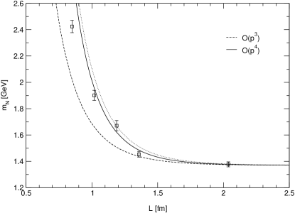
Figure 11: Volume dependence of the nucleon mass for $m_{\pi}=643$ MeV. The dashed curve represents the $O(p^{3})$ term only, while the solid curve also includes the $O(p^{4})$ contribution. The dotted curve results if the pion mass is reduced by 10% in the $O(p^{4})$ formula.

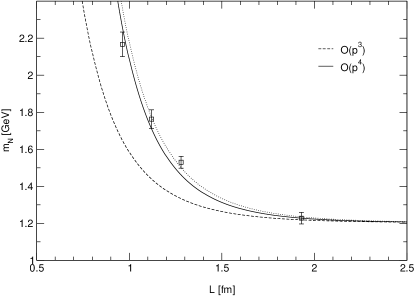
Figure 12: Same as Fig. 11 for $m_{\pi}=490$ MeV.

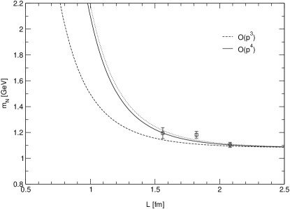
Figure 13: Same as Fig. 11 for $m_{\pi}=419$ MeV.

Using the parameters corresponding to the solid curve in Fig. 10 we can evaluate the finite-size formulae (II) and (7) and compare the results to our data. Our three sets of simulations with different lattice sizes correspond to pion masses of approximately 643, 490 and 419 MeV. Note that the latter two masses are lighter than the lightest of the pion masses investigated in Ref. Ali Khan et al. (2004) (732, 717 and 545 MeV). The curves in Figs. 11–13 have been computed from equations (II) and (7) with no free parameters. Like in Ref. Ali Khan et al. (2004) the solid curves correspond to the $O(p^{4})$ prediction

$$m_{N}(L)=m_{N}+\Delta_{a}(L)+\Delta_{b}(L),$$ (50)

where $m_{N}$ has been determined such that the calculated value $m_{N}(L_{\mathrm{max}})$ equals the simulated mass from the largest lattice with $L\!=\!L_{\mathrm{max}}$, respectively. Correspondingly, for the pion masses $m_{\pi}$ we also take the simulated value from the largest lattices. For the dashed curve, corresponding to the $O(p^{3})$ prediction, the $O(p^{4})$ contribution from $\Delta_{b}$ in (50) has been omitted, while $m_{N}$ has been left unchanged. For all our pion masses we find a surprisingly good overall description of our data by the $O(p^{4})$ prediction even down to lattice sizes of about 1 fm. Replacing $m_{\pi}$ from the largest, $L\!=\!16$ lattice at $(\beta,\kappa)=(5.32144,0.1665)$ by the mean of the pion masses from the $L=12,14,16$ lattices (as we did in Fig. 10) does not lead to a significant difference in the resulting curve. Since both the statistical and the theoretical errors of the simulated $m_{N}(L)$ are smallest for the largest lattice, we consider the $O(p^{4})$ finite-size corrected nucleon mass

$$\tilde{m}_{N}(L)=m_{N}(L)-\Delta_{a}(L)-\Delta_{b}(L),$$ (51)

taken at $L\!=\!L_{\mathrm{max}}$, as our best estimate of the asymptotic nucleon mass. Table 9 shows the predicted infinite-volume masses for our simulations. The last column gives the relative mass shift on the largest lattice, respectively. Just as it was the case for the pion, the finite size effect in the nucleon at $(\beta,\kappa,L)=(5.6,0.1575,24)$ is considerably smaller than the statistical uncertainty. At $(\beta,\kappa,L)=(5.6,0.158,24)$ and $(5.32144,0.1665,16)$, on the other hand, the finite-size effects according to Eq. (51) amount to about 2% of the respective asymptotic mass, which is comparable to the statistical errors.

Table 9: Finite-size shifts of the nucleon masses on the largest lattices as inferred from Eq. (50). $\Delta=(m_{N}-\tilde{m}_{N})/\tilde{m}_{N}$ is the relative deviation of the Monte Carlo value $m_{N}$ from the shifted mass $\tilde{m}_{N}=m_{N}-\Delta_{a}-\Delta_{b}$ (all values to be taken at $L_{\mathrm{max}}$). We consider $\tilde{m}_{N}(L_{\mathrm{max}})$ as the best estimate of the true asymptotic mass.

$\beta$	$\kappa$	$m_{\mathrm{PS}}\,[\mathrm{GeV}]$	$\tilde{m}_{N}(L_{\mathrm{max}})\,[\mathrm{GeV}]$	$m_{N}(L_{\mathrm{max}})\,[\mathrm{GeV}]$	$\Delta$
5.6	0.1575	0.6429(67)	1.370(19)	1.377(19)	0.53%
	0.1580	0.4896(94)	1.204(31)	1.228(31)	2.02%
5.32144	0.1665	0.4188(75)	1.081(20)	1.104(20)	2.08%

Compared to a fit-based extrapolation the advantage of a formula without free parameters is of course that one can directly calculate the amount by which one has to shift the nucleon mass in order to compensate for the finite-size effect associated with a given volume, and that one has control over the error. In practice, however, a remaining caveat is that the infinite-volume pion mass must be known. If one is working in a parameter regime where the finite-size effect in the pion mass is small (of the order of a few percent) one can apply the results of Ref. Colangelo and Dürr (2004) to obtain an estimate of the true asymptotic mass. If this is unclear, but data from several (more than two) different volumes are available, one might still revert to an exponential fit and extrapolate. Since we have seen that such a “naive” extrapolation systematically underestimates the true infinite-volume pion mass we illustrate, as an example, the impact of a by 10% smaller pion mass by the dotted curves in Figures 11–13. Although relative to the very nucleon mass shift the systematic error associated with the uncertainty in the pion mass grows with $L$, its absolute value becomes less and less significant compared to the statistical errors of the data. On the one hand this means that (assuming the formula to exactly reproduce the volume dependence of the data and the statistical uncertainties to be all of comparable size) in order to predict the asymptotic nucleon mass correctly (within the statistical errors) one needs to know $m_{\pi}$ the more accurately the smaller the physical size of the largest available lattice. If, on the other hand, $L$ is sufficiently large so that one can reliably extrapolate the pion mass, the asymptotic nucleon mass can be determined quite accurately, already on the basis of a single lattice.

V.3 Spatial Polyakov-type loops

At our two larger quark masses we have observed in all considered quantities (pion, rho and nucleon masses, pion decay constant) a drastic increase of the finite-size shifts below a lattice size of approximately 1.5 fm. But above this size the finite-size effects are relatively small, also at our smallest quark mass. As we will now show, this kind of transition behavior is reflected in the behavior of spatial Polyakov-type loops.

In the absence of dynamical quarks, i.e. in quenched QCD, the expectation value of the Polyakov loop, which is defined as

$$\bigl{\langle}{P}\bigr{\rangle}=\left\langle\frac{1}{L^{3}}\sum_{\mathbf{x}}\mathrm{Tr}\prod_{\tau=1}^{T}U_{4}(\mathbf{x},\tau)\right\rangle,$$ (52)

is zero in the confined phase, while in the deconfined phase $\left\langle{P}\right\rangle\neq 0$. Therefore in pure gauge theory $\left\langle{P}\right\rangle$ is an order parameter for the deconfining phase transition. This is due to the global $Z(3)$ symmetry of the pure $SU({3})$ gauge theory which is spontaneously broken at the phase transition. In full QCD the Polyakov loop is not an order parameter because the $Z(3)$ symmetry of the gluonic action is explicitly broken by the quark action, so that $\left\langle{P}\right\rangle$ is not exactly zero in the hadronic phase. In our simulations it is not the time extent $T$ which is varied, but the spatial lattice size $L$. Due to the space-time symmetry of the Euclidean metric, however, similar considerations also apply to Polyakov-type loops in the spatial directions (also known as Wilson lines). Let us, for definiteness, consider the mean Wilson line in $z$-direction, which is defined configuration-wise as

$$P_{z}=\frac{1}{L^{2}T}\sum_{x_{1},x_{2},\tau}\mathrm{Tr}\prod_{x_{3}=1}^{L}U_{3}(x_{1},x_{2},x_{3},\tau).$$ (53)

Table 10: Ensemble averages of the real and imaginary parts of the mean spatial Polyakov loop (in $z$-direction).

$\beta$	$\kappa$	$L^{3}T$	$\bigl{\langle}{\mathrm{Re}\,P_{z}}\bigr{\rangle}$	$\bigl{\langle}{\mathrm{Im}\,P_{z}}\bigr{\rangle}$
5.32144	0.1665	$12^{3}32$	-0.00056433(3)	-0.0003573(2)
		$14^{3}32$	-0.0000179(2)	-0.00003209(4)
		$16^{3}32$	0.00012251(3)	-0.00021856(4)
5.6	0.1575	$10^{3}32$	-0.0131032(3)	-0.006341(8)
		$12^{3}32$	-0.0029148(3)	0.0012405(6)
		$14^{3}32$	-0.00083854(3)	0.00008748(3)
		$16^{3}32$	0.00020948(3)	0.00004254(5)
		$24^{3}40$	-0.000078415(8)	-0.00009462(1)
	0.1580	$12^{3}32$	-0.003798(2)	0.005014(3)
		$14^{3}32$	-0.00135725(6)	0.0003214(3)
		$16^{3}32$	-0.00037040(4)	-0.00022400(4)
		$24^{3}40$	-0.00010810(2)	0.00012503(1)

As can be seen from Table 10, the expectation values $\left\langle{P_{z}}\right\rangle$ for all GRAL simulations are indeed significantly different from zero, even on the largest lattices. While for the larger lattices the deviation from zero is relatively small it becomes more pronounced as the lattices shrink. $\left\langle{\mathrm{Re}\,P_{z}}\right\rangle$ in particular takes increasingly negative values towards the smaller volumes. This can be understood by looking at the distribution of $P_{z}$.

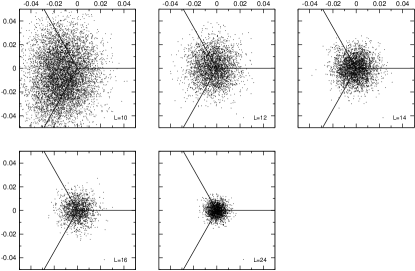
Figure 14: Distribution in the complex plane of the spatial Polyakov loop $P_{z}$ for the different lattices simulated at $(\beta,\kappa)=(5.6,0.1575)$. The lines indicate the three $Z(3)$ directions $1$, $e^{2\pi i/3}$ and $e^{4\pi i/3}$.

Fig. 14 shows the distribution in the complex plane of $P_{z}$ for the lattice volumes simulated at $(\beta,\kappa)=(5.6,0.1575)$. The lines in the plots indicate the three $Z(3)$ directions $1$, $e^{2\pi i/3}$ and $e^{4\pi i/3}$. Apart from the $L$-dependent fluctuations we observe for the larger lattices an approximately point-symmetric accumulation of the Wilson line around zero. This is reflected in the smallness of $\lvert{\left\langle{P_{z}}\right\rangle}\rvert$ and the corresponding statistical errors at large $L$ (Table 10). The situation is somewhat different for the smallest, $10^{3}$ lattice, where the distribution of Wilson lines is visibly shifted towards the $Z(3)$ directions $e^{2\pi i/3}$ and $e^{4\pi i/3}$, which leads to the relatively large negative value of $\left\langle{\mathrm{Re}\,P_{z}}\right\rangle$.

This shift can be understood e.g. by means of the 3-d Potts model with magnetic field that is recovered when the full QCD action is expanded first in the gauge coupling $\beta$ and then in inverse powers of the sea quark mass Antonelli et al. (1995). Introducing the quark action in QCD is then equivalent to switching on a magnetic field $h$ in the Potts model that breaks the $Z(3)$ symmetry of the system. Considering the phase of the spatial Polyakov loop as a spin that can take one of the three possible values $1$, $e^{2\pi i/3}$ and $e^{4\pi i/3}$, the magnetic field aligns the spins to preferred directions depending on the sign of $h$: for $h=-\lvert{h}\rvert$ (corresponding to antiperiodic spatial boundary conditions for sea quarks) the positive real axis is favored, whereas for $h=+\lvert{h}\rvert$ (periodic spatial boundary conditions for sea quarks) the two directions $e^{2\pi i/3}$ and $e^{4\pi i/3}$ (pointing towards negative values) are preferred. If we recall that we have used periodic spatial boundary conditions for sea quarks this explains the plot for $L=10$ in Fig. 14.

The implications of such a shift for finite-size effects in hadron masses have been explained in detail e.g. by Aoki et al. in the context of their comparative study of finite-size effects in quenched and full QCD simulations Aoki et al. (1994a). We briefly recapitulate their argument for our choice of boundary conditions: Let us consider a meson propagator $\Gamma(\tau)$ on a lattice of size $L^{3}$ with a sufficiently large time extent $T$. A hopping parameter expansion of $\Gamma(\tau)$ yields a representation of the meson propagator in terms of closed valence quark loops $C$ going through the meson source and sink. If we denote the corresponding link factors $\operatorname{Tr}\prod_{l\in C}U_{l}$ by $P(C)$ for Polyakov-type loops that wind around the lattice in a spatial direction, and $W(C)$ for ordinary Wilson-type loops, the meson propagator can be written as

$$-\bigl{\langle}{\Gamma(\tau)}\bigr{\rangle}=\sum_{C}\kappa_{\mathrm{val}}^{L(C)}\bigl{\langle}{W(C)}\bigr{\rangle}+\sum_{C}\kappa_{\mathrm{val}}^{L(C)}\sigma_{\mathrm{val}}\bigl{\langle}{P(C)}\bigr{\rangle},$$ (54)

where $L(C)$ is the length of the respective loop and the sign factor $\sigma_{\mathrm{val}}$ is equal to $+1$ for the periodic spatial boundary conditions used for valence quarks in our simulations. From the discussion above we know that in the case of periodic spatial boundary conditions for both sea and valence quarks the contribution of Polyakov-type loops to the meson propagator (54) is negative. Since mean values of Wilson-type loops are always positive, the two contributions in (54) have opposite sign, which leads to a faster decrease of the correlator and thus to a larger meson mass.

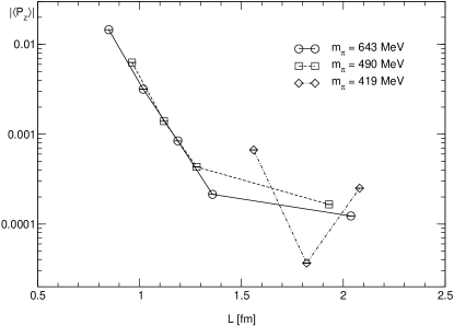
Figure 15: Absolute values of the complex ensemble averages of the spatial Polyakov loop $P_{z}$.

For fixed sea and valence quark mass this effect grows weaker for increasing lattice size because the contribution of the Polyakov-type loops decreases. This can clearly be seen from Fig. 15 for our larger pion masses. On the other hand, in a fixed lattice volume with periodic boundary conditions finite-size effects in hadron masses get increasingly significant both for decreasing sea and valence quark mass. This has been observed e.g. in Ref. Eicker (2001), where partially quenched chiral extrapolations of the pseudoscalar and vector masses were studied for the various sea and valence quark masses at $\beta=5.5$ and $5.6$. The sea quark mass dependence of the expectation value of the Wilson line can also be seen in Table 10 if one compares at $\beta=5.6$ the value for a given lattice size at $\kappa=0.1575$ with the corresponding value at $\kappa=0.158$. We find that in the same volume $\left\langle{\mathrm{Re}\,P_{z}}\right\rangle$ is more negative for the larger $\kappa$, corresponding to a smaller quark mass. This leads to a stronger cancellation of the two terms in (54) and hence to a larger finite-size effect in the hadron masses.

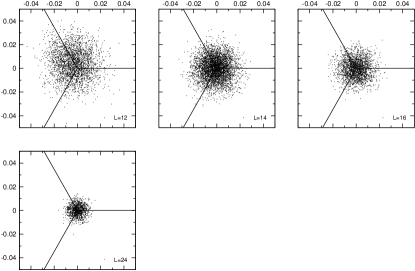
Figure 16: Same as Fig. 14 for $(\beta,\kappa)=(5.6,0.158)$.

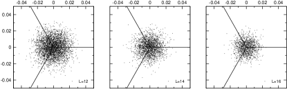
Figure 17: Same as Fig. 14 for $(\beta,\kappa)=(5.32144,0.1665)$.

For completeness, Figs. 16 and 17 show the distribution of the Wilson line for the simulated volumes at $(\beta,\kappa)=(5.6,0.158)$ and $(5.32144,0.1665)$.

VI Discretization Errors

One method that lends itself to checking on the significance of lattice artefacts in our simulations is to consider the PCAC relation

$$\partial_{\mu}A_{\mu}^{a}(x)=2mP^{a}(x)$$ (55)

between the isovector axial current

$$A_{\mu}^{a}(x)=\overline{q}(x)\gamma_{\mu}\gamma_{5}\frac{1}{2}\tau^{a}q(x)$$ (56)

and the associated density

$$P^{a}(x)=\overline{q}(x)\gamma_{5}\frac{1}{2}\tau^{a}q(x),$$ (57)

where $\tau^{a}$ denotes a Pauli matrix acting on the flavor indices of the quark field $q$. On the lattice, the bare quark mass $Z_{q}M_{q}$ can be extracted from ratios of correlation functions,

$$Z_{q}M_{q}=\frac{1}{2}\frac{\bigl{\langle}{\partial_{\mu}A_{\mu}^{a}(x)J^{a}}\bigr{\rangle}}{\bigl{\langle}{P^{a}(x)J^{a}}\bigr{\rangle}}+O(a),$$ (58)

where the (smeared) source $J^{a}$ is a suitable polynomial in the quark and gluon fields, and $Z_{q}\!=\!Z_{P}/Z_{A}$. The PCAC relation (55) is an operator identity that holds for the Wilson action up to $O(a)$ effects. Consequently, its lattice version holds—up to those effects—for any choice of boundary conditions, source operators and lattice sizes. This means in particular that at fixed $\beta$ and $\kappa$ any residual lattice size dependence of the PCAC quark mass (58) must be a lattice artefact. Figs. 18–20 show the volume dependence of the relative deviation of the PCAC quark mass $m_{q}(L)$ from its value $m_{q}$ on the largest lattices, for our three $(\beta,\kappa)$ combinations.

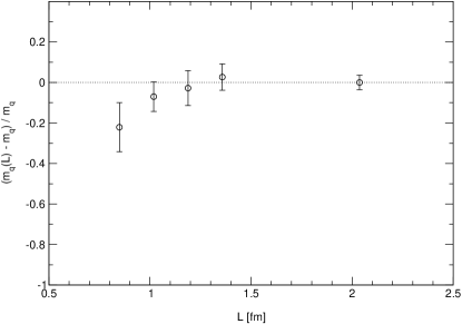
Figure 18: Box-size dependence of the relative shift in the PCAC quark mass at $(\beta,\kappa)=(5.6,0.1575)$.

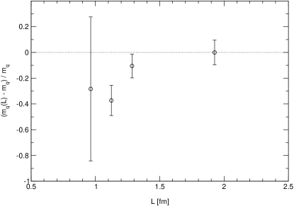
Figure 19: Same as Figure 18 for $(\beta,\kappa)=(5.6,0.158)$.

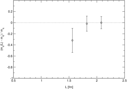
Figure 20: Same as Figure 18 for $(\beta,\kappa)=(5.32144,0.1665)$.

We find that at $(\beta,\kappa)=(5.6,0.1575)$ the discretization errors appear to be small for $L\gtrsim 1$ fm, while for $(\beta,\kappa)=(5.6,0.158)$ and $(5.32144,0.1665)$ they are small only for $L\gtrsim 1.3$ fm and $L\gtrsim 1.8$ fm, respectively. On the smaller lattices the cut-off shows up in quark mass shifts of 20–40% (with large error bars on the smallest lattices). The fact that the cut-off effects are small for $(\beta,\kappa)=(5.6,0.1575)$ and somewhat larger for $(\beta,\kappa)=(5.6,0.158)$ and $(5.32144,0.1665)$ is consistent with our observations in Section V, where in Fig. 10 we saw no significant lattice artefacts in the nucleon mass for $m_{\pi}=643$ MeV, while for $m_{\pi}=490$ MeV and $m_{\pi}=419$ MeV the nucleon mass displayed some deviation from the curve (which represents a fit to $O(a)$-improved data).

VII Summary

In order to investigate finite-size effects in stable light hadron masses obtained from Lattice QCD with two dynamical flavors of Wilson fermions we have complemented previous SESAM/T$\chi$L simulations at quark masses corresponding roughly to 85 and 50% of the strange quark mass by several runs at the same coupling of $\beta=5.6$, but on smaller lattices. In addition we have carried out exploratory simulations using three different lattice volumes at a stronger coupling of $\beta=5.32144$ in an attempt to push our analysis towards the regime of lighter quark masses. We have succeeded in simulating near $m_{s}/3$, which in terms of $m_{\pi}/m_{\rho}$ is close to the rho decay threshold of $0.5$. The physical extent of the investigated lattices ranges between 0.85 fm and 2.04 fm.

We have addressed, from a practical point of view, the question to what extent the volume dependence of the computed pion, rho and nucleon masses can be parameterized by simple functions, and if with these functions an extrapolation from small and intermediate lattices to the infinite volume is possible. To this end we have compared an exponential ansatz motivated by Lüscher’s mass-shift formula for the pion to the power law observed by Fukugita et al.. On the basis of various fits we conclude that while the power law may be used to describe the volume dependence of the masses at volumes smaller than roughly $(1.5~{}\mathrm{fm})^{3}$, over the full range of simulated lattices—and in particular with respect to the asymptotic behavior—the exponential ansatz is more appropriate. Although the extrapolation of simple exponential fits to the infinite volume in general provides only a lower bound to the asymptotic mass, this bound may be close to the true asymptotic value if the relative difference between the masses from the largest volumes incorporated in the fit is already quite small (of the order of a few percent). For small volumes alone, however, this is in general not the case.

The exponential parameterization corresponds in its functional form precisely to Lüscher’s asymptotic formula for the pion (with input from infinite-volume ChPT at leading order). Although we have found that the single exponential allows for a reasonable phenomenological description of our light hadron masses over a wide range of lattice volumes, a large coefficient multiplying the exponential attests to the fact that the data points from the small lattices lie outside the parameter regime in which the original formula holds. In the case of the pion we have illustrated this by a comparison of our data to Lüscher’s formula with input from ChPT up to NNLO and to the full LO ChPT result for the pion mass in finite volume. Of course, if an appropriate analytic prediction with controlled errors is available it is preferable to an extrapolation based on a fit with free parameters. We have found, however, that in the parameter regime of our simulations even the best currently available estimate for the pion finite-size effect, based on a combination of the asymptotic Lüscher formula with NNLO ChPT input and the full finite-volume (but LO) ChPT result, predicts mass shifts of a few percent only. This is comparable in size to the typical statistical errors and therefore hard to detect in practice. Our simulations at $\beta=5.32144$ probably are in a pion mass regime where the box-size dependence can be described by such a formula, but more statistics is needed to corroborate this assumption. While Lüscher’s formula with input at next-to-leading and next-to-next-to-leading order ChPT can be used to control the convergence of the chiral expansion, a full higher order result from ChPT for the pion mass in finite volume would be highly useful to fully assess the role of the sub-leading terms in the large-$L$ expansion.

For the nucleon, a promising finite-size mass formula has recently become available from relativistic Baryon ChPT. We have shown for three different pion masses (two of which are smaller than the ones considered by the QCDSF-UKQCD collaboration) that it describes our simulated nucleon masses remarkably well even down to box-sizes of about 1 fm. We have also seen that above this size it can, in principle, be used to estimate the infinite-volume mass already on the basis of a single measurement, provided that the corresponding asymptotic pion mass is known. If, as in our case, data from several lattice volumes are available, they can be combined to obtain a reliable estimate with controllable errors.

*

Appendix A Fit parameters

Table 11: Fit parameters for $(\beta,\kappa)=(5.6,0.1575)$. $d=2$ for “pow” (Eq. (39)) and $d=1/2$ for “exp” (Eq. (38)).

Fit type	$H$	$[L_{1},L_{2}]$	$m_{H}\,[\mathrm{GeV}]$	$c\,[\mathrm{GeV}^{-d}]$	$\chi^{2}/\mathrm{df}$	$\Delta(L_{\mathrm{max}})$	$\Delta(L\!=\!\infty)$
pow	PS	$10,24$	0.570(35)	41.2(7.1)	31.65	-5.57%	-11.40%
pow	V	$10,24$	0.872(19)	35.1(5.3)	3.34	-1.38%	-4.87%
pow	N	$10,24$	1.255(43)	88.5(9.3)	5.83	-2.99%	-8.84%
exp	PS	$10,24$	0.624(13)	65.9(4.2)	5.59	-2.41%	-2.91%
exp	V	$10,24$	0.9125(92)	63.5(5.6)	1.19	-0.17%	-0.51%
exp	N	$10,24$	1.372(22)	142.7(9.5)	2.37	0.18%	-0.32%

Table 12: Same as Table 13 for $(\beta,\kappa)=(5.6,0.158)$.

Fit type	$H$	$[L_{1},L_{2}]$	$m_{H}\,[\mathrm{GeV}]$	$c\,[\mathrm{GeV}^{-d}]$	$\chi^{2}/\mathrm{df}$	$\Delta(L_{\mathrm{max}})$	$\Delta(L\!=\!\infty)$
pow	PS	$12,24$	0.417(33)	55.3(9.2)	8.55	-2.67%	-14.81%
pow	V	$12,24$	0.780(59)	62.5(13.1)	5.22	-2.10%	-9.86%
pow	N	$12,24$	1.0894(92)	124.0(2.3)	0.07	-0.44%	-11.30%
exp	PS	$12,24$	0.466(20)	47.9(4.2)	3.86	-1.50%	-4.91%
exp	V	$12,24$	0.836(45)	53.1(10.0)	4.31	-1.27%	-3.41%
exp	N	$12,24$	1.208(20)	104.1(5.1)	0.50	1.30%	-1.65%

Table 13: Same as Table 13 for $(\beta,\kappa)=(5.32144,0.1665)$.

Fit type	$H$	$[L_{1},L_{2}]$	$m_{H}\,[\mathrm{GeV}]$	$c\,[\mathrm{GeV}^{-d}]$	$\chi^{2}/\mathrm{df}$	$\Delta(L_{\mathrm{max}})$	$\Delta(L\!=\!\infty)$
pow	PS	$12,16$	0.428(22)	-15.0(16.3)	2.09	-0.83%	2.23%
pow	V	$12,16$	0.743(32)	23.3(29.0)	0.77	0.54%	-2.08%
pow	N	$12,16$	1.037(63)	90.9(52.8)	1.87	0.98%	-6.05%
exp ($c\!=\!C$)	PS	$12,16$	0.4089(81)		2.04	-2.36%	-2.36%
exp	V	$12,16$	0.756(20)	18.4(26.7)	0.86	0.64%	-0.31%
exp	N	$12,16$	1.088(42)	74.9(50.5)	2.32	1.19%	-1.46%