Finite volume effects
for meson masses and decay constants

Abstract

We present a detailed numerical study of finite volume effects for masses and decay constants of the octet of pseudoscalar mesons. For this analysis we use chiral perturbation theory and asymptotic formulae à la Lüscher and propose an extension of the latter beyond the leading exponential term. We argue that such a formula, which is exact at the one-loop level, gives the numerically dominant part at two loops and beyond. Finally, we discuss the possibility to determine low energy constants from the finite volume dependence of masses and decay constants.

1 Introduction

In lattice QCD the determination of the mass and decay constant of the lowest-lying state with a given set of quantum numbers is entering the high-precision era. Even in the fully unquenched case (i.e. with sea- and valence-quarks being degenerate) the pion mass can be measured, for fixed bare parameters, with an accuracy at the percent level, and future progress towards the permille level is anticipated. However, to make contact with the real world, three extrapolations are needed. These are $(i)$ the continuum extrapolation, $(ii)$ the infinite volume extrapolation, and $(iii)$ the chiral extrapolation. In each case there is considerable help and an analytical guideline from an effective field theory framework.

This article is concerned with the extrapolation to infinite volume, where the situation is particularly favorable (for a compact review of the recent literature see [2]). As shown by Gasser and Leutwyler, chiral symmetry imposes strong constraints on the dynamics at low energy in QCD, even if the system is enclosed in a finite box. Accordingly, Chiral Perturbation Theory (ChPT) may be adapted to the finite volume case [3, 4, 5]. In this framework finite volume effects can be taken systematically into account, in a perturbative loop expansion. If the spatial volume $L^{3}$ is large enough internal degrees of freedom of the particle of interest play no role as far as finite volume effects are concerned and these are exclusively due to pion loops. This means that they first appear at next-to-leading order (NLO), i.e. at $O(p^{4})$ in the chiral counting. Another consequence is that they are exponentially small in the pion mass for any particle that couples to the pion field: the effect behaves like $e^{-M_{\pi}L}$ for pions, kaons, etas and nuclei. To date, a number of finite volume calculations have been performed at one-loop order. In the nucleon sector the corrections to the mass [6, 7], the magnetic moment [7] and the baryon axial charge [8] have been worked out. In the meson sector the original calculation for $M_{\pi}(L)$ and $F_{\pi}(L)$ [3] has been extended to the quenched case [9]. The same quantities have also been analyzed in a quark-meson model [10]. More recently, the finite volume shifts for $F_{K}(L)$ and $B_{K}(L)$ have been given in Ref. [11] and the extension to heavy-meson chiral perturbation theory has been described [12]. No full two-loop calculation of finite volume effects has appeared yet.

For some observables the Lüscher formula represents a convenient and powerful alternative [13]. It allows to estimate subleading (in the chiral counting) finite volume effects for the mass of a particle with less effort, while sticking to the leading order in an expansion in powers of $e^{-M_{\pi}L}$. The formula gives the finite volume shift $M_{P}(L)\!-\!M_{P}$ of a particle $P$ in terms of the infinite volume $\pi P$ forward scattering amplitude in the unphysical (Euclidean) region. For this amplitude the ChPT expression at a certain loop order is used. The approach via the Lüscher formula is economical, since only a chiral calculation in infinite volume is needed, and the loop in finite volume comes for free. Applications of the Lüscher formula to the mass of the nucleon [6, 14] and the pion [15] have been worked out. In the latter publication several orders in the ChPT input for the $\pi\pi$ scattering amplitude were compared and it was found that in a certain range of $M_{\pi}$ and $L$ subleading effects (in the chiral counting) can be large with respect to the leading contributions. An extension of the Lüscher formula has been constructed for pseudoscalar decay constants [16].

This article presents a resummed version of the Lüscher formulae for masses and decay constants (this has been briefly discussed by one of us in [2]), where the terms neglected in the large-$L$ expansion are $\sim\!e^{-(\sqrt{3}+1)/\sqrt{2}\cdot M_{\pi}L}$, rather than $e^{-\sqrt{2}M_{\pi}L}$. We proceed with the asymptotic expression for $M_{\pi}(L)\!-M_{\pi}$ to 3-loop order, and for $F_{\pi}(L)\!-\!F_{\pi},M_{K}(L)\!-\!M_{K},F_{K}(L)\!-\!F_{K}$ to 2-loop order, by using the available knowledge in the literature on the scattering amplitude or axial-vector matrix element. In all cases, the result may be given in a compact formula that does not involve any numerical integration.

2 Finite volume effects

Lattice calculations are necessarily done in a finite 4D volume which acts as an IR-cutoff. Typically a $L^{3}\!\times\!T$ geometry with periodic boundary conditions in all directions is chosen with $T\!\gg\!L$ and both large compared to the inverse temperature of the QCD phase transition or crossover. In order to determine the mass of a particle one considers a correlator of two properly chosen interpolating fields

$$C(t)=\int d^{3}x\;\langle\phi(x)\phi(0)\rangle\;e^{\mathrm{i}\mathbf{px}}\;\;\stackrel{{\scriptstyle T\to\infty}}{{\longrightarrow}}\;\;\sum_{n=0}^{\infty}c_{n}\,e^{-E_{n}t}$$ (1)

and tries to determine the energy levels (typically the lowest) at zero spatial momentum, $M_{n}(L)=E_{n}(\mathbf{p}=0)$. In the following, we will be concerned with the shift $M(L)-M$, where $M\!\equiv\!M(L\!=\!\infty)$, for the groundstate ($n\!=\!0$) due to the finite 3D volume $L^{3}$. Decay constants or, more generally, matrix elements suffer from analogous shifts at finite spatial volume. For not-too-small box length $L$ these shifts can be calculated analytically, thus offering a means to correct lattice data for this systematic effect. We now give a brief outline of the two main frameworks for such a calculation. A comment on cut-off effects and their interplay with finite volume effects is given in appendix B.

2.1 ChPT in finite volume

In QCD with light flavors the physics in the infrared region is controlled by chiral symmetry. As shown by Gasser and Leutwyler this still holds true if the system is enclosed in a finite box $L^{3}\!\times\!T$, provided both $L$ and $T$ are large enough that chiral symmetry is not restored [5]. They have shown that in an isotropic box with periodic boundary conditions for the meson fields the finite-volume dependence comes in exclusively through the propagators. The latter becomes periodic in all spatial directions, and in the limit $T\to\infty$ can be written as follows

$$G(x^{0},\mathbf{x})=\sum_{\mathbf{n}}G_{0}(x^{0},\mathbf{x}+\mathbf{n}L)$$ (2)

which is equivalent to replacing the integration over the spatial part of the momenta by a sum over multiples of $2\pi/L$. In other words, with periodic boundary conditions the Lagrangian remains the same as in infinite volume.

The expansion parameters in ChPT are

$${p\over 4\pi F_{\pi}}\qquad,\qquad{M_{\pi}\over 4\pi F_{\pi}}$$ (3)

and the theory can be meaningfully applied only if both are small. In a finite volume spatial momenta are discretized: $\mathbf{p}=2\pi\mathbf{n}/L$ with $\mathbf{n}$ a vector of integers. Therefore one can have “small” nonzero momenta and apply ChPT only if the condition

$$L\!\gg\!{1\over 2F_{\pi}}\!\sim\!1\,\mathrm{fm}$$ (4)

is satisfied. A priori there is no way to say how much $L$ has to be in excess of 1 fm. As a guideline we observe that the lowest non-trivial momentum in a 1 fm box is $1.2\,\mathrm{GeV}$, which is certainly beyond the realm of ChPT. Note, finally, that unlike $F_{\pi}L$ the combination $M_{\pi}L$ is not constrained. Both $M_{\pi}L\!\ll\!1$ and $M_{\pi}L\!\gg\!1$ are acceptable [3, 4, 5, 17], but they imply different ways to organize the chiral series,

$$M_{\pi}L\gg 1\quad\leftrightarrow\quad\mbox{``$p$-expansion''}\,\,$$ (5)

$$M_{\pi}L\ll 1\quad\leftrightarrow\quad\mbox{``$\epsilon$-expansion''}\;.$$ (6)

Here we shall restrict ourselves to the former case, where the chiral counting is

$$M_{\pi}^{2}\sim m\sim O(p^{2}),\qquad 1/L\sim p\sim O(p)\;.$$ (7)

With this setup Gasser and Leutwyler calculated the mass and decay constant shift in a theory with $N_{\!f\,}^{2}\!-\!1$ degenerate pseudo-Goldstone bosons, and obtained [3]

$$M_{\pi}(L) = M_{\pi}\left[1+{1\over 2N_{\!f\,}}\xi_{\pi}\,\tilde{g}_{1}(\lambda_{\pi})+O(\xi_{\pi}^{2})\right]$$ (8)

$$F_{\pi}(L) = \;F_{\pi}\left[1-\;{N_{\!f\,}\over 2}\,\xi_{\pi}\,\tilde{g}_{1}(\lambda_{\pi})+O(\xi_{\pi}^{2})\right]\;.$$ (9)

Here we have introduced the abbreviations (note the $F_{\pi}$ in the denominator for all $P$)

$$\xi_{P} \equiv {M_{P}^{2}\over(4\pi F_{\pi})^{2}}$$ (10)

$$\lambda_{P} \equiv M_{P}L$$ (11)

for $P\!=\!\pi$ (and $P\!=\!K,\eta$ will be used below) as well as the modified shape function

$$\tilde{g}_{1}(x)=\sum_{n=1}^{\infty}{4m(n)\over\sqrt{n}\,x}\;K_{1}(\sqrt{n}\,x)$$ (12)

where $K_{1}$ is a Bessel function of the second kind and the multiplicities $m(n)$ have been given in [15], but for convenience we reproduce them in Tab. 1. Given the asymptotic expansion $K_{1}(z)\!\sim\!\sqrt{\pi/(2z)}e^{-z}$, it is clear that in the $p$-regime eqns. (8, 9, 12) represent quickly converging expressions. Several observables have been worked out at one-loop order [6, 7, 8, 9, 11, 12, 18, 19], but to date no two-loop result obtained in this setup has appeared.

$n$	1	2	3	4	5	6	7	8	9	10	11	12	13	14	15	16	17	18	19	20
$m(n)$	6	12	8	6	24	24	0	12	30	24	24	8	24	48	0	6	48	36	24	24

Table 1: The multiplicities $m(n)$ in (12) for $n\leq 20$.

2.2 Lüscher formula

An entirely independent approach has been devised by Lüscher who has proven an elegant relation between the mass shift of the particle $P$ in a finite volume $L^{3}\!\times\!\infty$ and the $P\pi$ scattering amplitude in infinite volume [13]

$$M_{P}(L)-M_{P}=-\,{3\over 16\pi^{2}\lambda_{P}}\;\int_{-\infty}^{\infty}\!dy\;\mathcal{F}_{P}(\mathrm{i}y)\,e^{-\sqrt{M_{\pi}^{2}+y^{2}}L}+O(e^{-\bar{M}L})\;.$$ (13)

Here $\mathcal{F}_{P}(\nu)$ denotes the infinite volume forward ($t\!=\!0$) scattering amplitude of $P$ and $\pi$ in Minkowski space. The integration runs along the imaginary axis, i.e. $\mathcal{F}_{P}(\nu)$ is evaluated for

$$\nu=\mathrm{i}y$$ (14)

with real $y$, thus staying far away from the cuts. Only the real part of $\mathcal{F}_{P}(\mathrm{i}y)$ contributes to the integral, since the imaginary part is odd in $y$. An additional piece in the original formula, referring to the 3-particle vertex, is omitted here, since we assume $P$ to be a pseudo-Goldstone boson. The Lüscher formula (13) keeps only the leading term in an expansion in (fractional) powers of $e^{-\lambda_{\pi}}$. The generic bound $\bar{M}\!\geq\!\sqrt{3/2}M_{\pi}$ can be specified to $\bar{M}\!=\!\sqrt{2}M_{\pi}$ in a theory with pseudo-Goldstone bosons only.

Recently, an analogous “Lüscher-type” formula has been derived for the finite volume shift of the axial-vector decay constant $F_{P}$. It reads [16]

$$F_{P}(L)-F_{P}=\,+{3\over 8\pi^{2}\lambda_{P}}\;\int_{-\infty}^{\infty}\!dy\;\mathcal{N}_{P}(\mathrm{i}y)\,e^{-\sqrt{M_{\pi}^{2}+y^{2}}L}+O(e^{-\bar{M}L})$$ (15)

where $\mathcal{N}_{P}(\nu)$ is derived from the matrix element $\langle\pi\pi|A_{\mu}|P\rangle$ via a subtraction prescription we will specify below. Like in the mass formula (13) the finite volume shift of $F_{P}$ is expressed in terms of an infinite-volume amplitude, evaluated in the unphysical (Euclidean) region, thus far away from the cuts. Again, only the leading term in an expansion in (fractional) powers of $e^{-\lambda_{\pi}}$ is kept. Note the reverse overall sign, compared to (13), and the fact that the net physical effect is opposite to this prefactor; in other words $M_{P}(L)\!>\!M_{P}$ and $F_{P}(L)\!<\!F_{P}$.

To predict the shifts $M_{P}(L)\!-\!M_{P}$ and $F_{P}(L)\!-\!F_{P}$ in a lattice calculation with a known box length $L$, and thus to correct the data for this systematic effect, the formulae (13, 15) must be fed with an explicit representation of the amplitudes $\mathcal{F}_{P}(\nu)$ and $\mathcal{N}_{P}(\nu)$, respectively. This is the place where ChPT naturally enters, even if one opts for the Lüscher approach. Using existing knowledge about the relevant amplitude at $n$-loop order, one gets the leading piece, in the $e^{-\lambda_{\pi}}$ expansion, of the finite-volume shift of $M_{P}(L),F_{P}(L)$ to $n\!+\!1$-loop order. For instance, using the tree-level expressions $\mathcal{F}_{\pi}(\nu)\!=\!-M_{\pi}^{2}/F_{\pi}^{2}$ and $\mathcal{N}_{\pi}(\nu)\!=\!-2M_{\pi}/F_{\pi}$ in 2-flavor ChPT yields

$$M_{\pi}(L)-M_{\pi} = +\,{3\over 8\pi^{2}}{M_{\pi}^{2}\over F_{\pi}^{2}L}\,K_{1}(\lambda_{\pi})+O(e^{-\sqrt{2}\lambda_{\pi}})$$ (16)

$$F_{\pi}(L)-F_{\pi} = -\,{3\over 2\pi^{2}}{M_{\pi}\over F_{\pi}L}\,K_{1}(\lambda_{\pi})+O(e^{-\sqrt{2}\lambda_{\pi}})$$ (17)

in agreement [3] with the 1-loop chiral expressions (8) and (9). Because of the “elevator”-effect in the loop expansion and since the associated chiral calculation is in infinite volume, it is much easier to push to higher chiral orders in the Lüscher-type setup than with a straightforward ChPT-in-finite-volume calculation [20]. This offers a genuine opportunity to compare several chiral orders and thus to assess the chiral convergence behavior. Indeed, in [15] the finite volume shift in the pion mass was evaluated, using ChPT at LO/NLO/NNLO for $\mathcal{F}_{\pi}(\nu)$ to get the asymptotic piece of the full chiral expression at 1/2/3-loop order, and it was found that for some $(M_{\pi},L)$-combinations the chiral series converges well, if at least the NLO input is included. Still, one might worry whether the non-asymptotic pieces of order $O(e^{-\sqrt{2}\lambda_{\pi}})$ would prove numerically relevant [20]. In [15] a first attempt was made to discriminate those regions in the $(M_{\pi},L)$-plane where higher orders in the chiral expansion dominate against those regions where terms omitted in the Lüscher approach are more important. Below, we shall present a resummed version of the Lüscher-type formulae (13, 15), where the pieces $\propto\!e^{-\sqrt{2}\lambda_{\pi}}$ and $\propto\!e^{-\sqrt{3}\lambda_{\pi}}$ are included and the terms $O(e^{-(\sqrt{3}+1)/\sqrt{2}\cdot\lambda_{\pi}})$ estimated. On this basis a more precise assessment of the relevance of higher loop corrections versus higher powers of $e^{-\lambda_{\pi}}$ can be made.

Note finally that all Lüscher-type formulae build on the unitarity of the theory and thus hold for the full (unquenched) theory. In the (partially) quenched case it seems indispensable to start in the framework of subsect. 2.1, but even then the arguments for using the infinite volume Lagrangian reside on less solid grounds – see Ref. [9] for a lucid discussion.

3 The Lüscher formula resummed

In Lüscher’s derivation of the asymptotic formula for the finite volume correction to particle masses the first step is a proof that the leading exponential term is given by the sum of all diagrams in which only one propagator is taken in finite volume. This class of diagrams yields

$$M_{P}(L)-M_{P}=-{1\over 4M_{P}}\sum_{\mathbf{n}\neq\mathbf{0}}\int\!\!{d^{4}q\over(2\pi)^{4}}\;e^{\mathrm{i}\mathbf{q}\cdot\mathbf{n}L}\,G_{0}(q)\Gamma(\hat{p},q,-\hat{p},-q)+\ldots$$ (18)

where $G_{0}(q)\!=\!1/(M_{\pi}^{2}+q^{2})$ is the full propagator and $\Gamma(p_{1},p_{2},p_{3},p_{4})$ the four-point vertex function in infinite volume. Lüscher then concentrates on the leading exponential contributions (those with $|\mathbf{n}|=1$), and shows that, if one disregards terms which are exponentially suppressed with respect to $\exp(-\lambda_{\pi})$, three of the four integrations in (18) can be performed explicitly and the result (13) is obtained. The same reasoning, however, applies also to all other terms in the sum in (18): for each of the terms with $|\mathbf{n}|>1$, one can obtain its leading exponential contribution by performing exactly the same steps that Lüscher did for the $|\mathbf{n}|=1$ term and work out three of the four integrations explicitly. It is easy to keep track of the vector $\mathbf{n}$ in doing these manipulations, and to get the resummed formula

$$M_{P}(L)-M_{P}=-\,{1\over 32\pi^{2}\lambda_{P}}\;\sum_{n=1}^{\infty}{m(n)\over\sqrt{n}}\int_{-\infty}^{\infty}\!dy\;\mathcal{F}_{P}(\mathrm{i}y)\,e^{-\sqrt{n(M_{\pi}^{2}+y^{2})}L}+O(e^{-\bar{M}L})$$ (19)

where $m(n)$ has been given in Tab. 1 and $\mathcal{F}_{P}(\nu)$ is the $P\pi$ forward scattering amplitude as usual. The extension which we are proposing is done in the same spirit as the extension of the domain of integration in (19) to infinity (the contributions from the region $|y|>\sqrt{\bar{M}^{2}\!-\!M_{\pi}^{2}}$ are beyond the accuracy of the formula): being of “kinematical” nature, the extension comes at no cost and may be numerically relevant. In this case, actually, one even obtains an improvement in the algebraic accuracy of the formula: we now have $\bar{M}>\sqrt{3}M_{\pi}$ and not, as before, $\bar{M}\!=\!\sqrt{2}M_{\pi}$. In other words, the terms $O(e^{-\sqrt{2}\lambda_{\pi}})$ and $O(e^{-\sqrt{3}\lambda_{\pi}})$ are included now. To further clarify the meaning of (19) let us list the two main classes of exponentially suppressed contributions which are still missing:

1. All diagrams which have more than one pion loop in finite volume. Obviously, these contributions start at the two-loop level in the chiral expansion.

2. Contributions to the integral (18) which are due to singularities in either the propagator $G_{0}$ or the vertex function $\Gamma$ which are further away from the real axis than $M_{\pi}$. These singularities show up only if one considers the vertex function at one loop, or the propagator at two-loop accuracy and beyond. All these contributions appear only if one calculates finite-volume effects at the two-loop level in the chiral expansion.

In the first class we distinguish those diagrams where different loops factorize (i.e. loops which have no propagator in common) from those which do not. It is easy to see that the former sub-class yields corrections of order $e^{-2\lambda_{\pi}}$. For two-loop diagrams which do not factorize (e.g. the two-loop sunset diagram) on may rely on the general discussion by Lüscher (cf. in particular Eqn. (2.49) in Ref. [13]) and conclude that the sunset diagram decays exponentially at large $L$ as $\exp(-N_{\mathrm{\tiny sunset}}\lambda_{\pi})$ with $N_{\mathrm{\tiny sunset}}=(\sqrt{3}\!+\!1)/\sqrt{2}\simeq 1.93$. For the second class we remark that the singularities neglected in (19) are due to the exchange of at least two pions, hence starting at $\nu\!=\!\pm 2M_{\pi}$, and this gives terms of order $e^{-2\lambda_{\pi}}$. We have not tried to prove the statement that the algebraic accuracy of our formula is given by

$$\bar{M}\!=\!M_{\pi}(\sqrt{3}\!+\!1)/\sqrt{2}$$ (20)

beyond the two-loop level, since it appears to us to be a question of academic interest.

More interesting is the question of how accurate the formula (19) is numerically. A complete analysis of finite-volume effects for $M_{\pi}$ and $F_{\pi}$ at the two loop level, which is currently under way [21], will clarify this point. The partial results we have so far indicate that the formula is very accurate. We have tried to find an algebraic reason for this, and found out that at the two loop level all diagrams which do not appear in Eq. (19) are suppressed (besides an extra exponential factor) by some power of $1/L$. The numerical results, however, seem to go beyond what one would expect from such an argument.

An analogy to the low-temperature expansion seems more suggestive. In the effective theory the large volume and the low temperature expansions are in one-to-one correspondence [5]. In Ref. [22] Schenk discussed the propagation of pions through matter in a state of thermal equilibrium at inverse temperature $\beta$. If the temperature is not too high, the hadronic phase mainly consists of pions, with effects of other excitations such as $K,\eta,\rho...$ exponentially suppressed. Due to interactions with pions of the heat bath, the effective pion mass $M_{\pi}(\beta)$ is given by [22]

$$M_{\pi}(\beta)-M_{\pi}=-{1\over 2M_{\pi}}\int\!\!{d^{3}q\over(2\pi)^{3}2\omega_{q}}\;n_{\mathrm{B}}(\omega_{q})\;T^{I=0}_{\pi\pi}(s)+O(n_{\mathrm{B}}^{2})$$ (21)

with $\omega_{q}=\sqrt{M_{\pi}^{2}+\mathbf{q}^{2}}$ and the density $n_{\mathrm{B}}(x)\!=\!1/(e^{\beta x}-1)$. The details of the pion kinematics will be discussed in the next section, and the isospin index refers to the $t$-channel. One immediately verifies that (21) agrees with the modified Lüscher formula in one dimension to first order in the density $n_{\mathrm{B}}$ – the density factor $n_{\mathrm{B}}$ in the integrand is the outcome of the resummation over $\mathbf{n}$ in (18) if $\mathbf{n}$ is taken as a one-dimensional vector. Schenk has carried the expansion of (21) one step further and determined the contributions of order $n_{\mathrm{B}}^{2}$ to the pion mass at finite temperature: in this extension, effects generated by three-body collisions are explicitly accounted for. It turned out that these effects are numerically very small, in line with intuition – the rescattering of three pions into three pions is a rare process unless the density is very high. Although the argument cannot be formulated in the same way for the finite volume case, we do see that the outcome of the numerical analysis is the same.

4 Meson masses and decay constants in finite volume

We start with the resummed Lüscher formulae for the relative finite-size shift of pseudoscalar masses and decay constants

$$R_{M_{P}}\equiv{M_{P}(L)-M_{P}\over M_{P}}\! \!=\! \!-\frac{M_{\pi}}{32\pi^{2}M_{P}\lambda_{P}}\sum_{n=1}^{\infty}\frac{m(n)}{\sqrt{n}}\int_{-\infty}^{\infty}\!d\tilde{y}\,\,\mathcal{F}_{P}(\mathrm{i}\tilde{y})e^{-\sqrt{n(1+\tilde{y}^{2})}\,\lambda_{\pi}}+O(e^{-\bar{M}L})\qquad$$ (22)

$$R_{F_{P}}\equiv\,\,\,{F_{P}(L)-F_{P}\over F_{P}}\! \!=\! \!+\,\frac{M_{\pi}}{16\pi^{2}F_{P}\lambda_{P}}\,\sum_{n=1}^{\infty}\frac{m(n)}{\sqrt{n}}\int_{-\infty}^{\infty}\!d\tilde{y}\,\mathcal{N}_{P}(\mathrm{i}\tilde{y})e^{-\sqrt{n(1+\tilde{y}^{2})}\,\lambda_{\pi}}+O(e^{-\bar{M}L})\qquad$$ (23)

where all symbols on the r.h.s. refer to infinite volume quantities. The multiplicities $m(n)$ are given in Tab. 1, $\lambda_{P}$ has been defined in (11), and the dimensionless integration variable (which we will be using from here on) relates to the previous one via $\tilde{y}\!=\!y/M_{\pi}$. The amplitudes $\mathcal{F}_{P}(\tilde{\nu}),\mathcal{N}_{P}(\tilde{\nu})$ with $\tilde{\nu}\!=\!\nu/M_{\pi}$ are

$$\mathcal{F}_{P}(\tilde{\nu})\! \!=\! \!T^{I=0}_{\pi P}(0,-4M_{P}\nu)$$

$$\mathcal{N}_{P}(\tilde{\nu})\! \!=\! \!-\mathrm{i}\bar{A}^{I=0}_{P}(0,-4M_{P}\nu)$$ (24)

where $T^{I=0}_{\pi P}(t,u\!-\!s)$ is the $P\pi$-scattering amplitude with zero $t$-channel isospin, and $\bar{A}^{I=0}_{P}(t,u\!-\!s)$ is the subtracted amplitude for the decay of the meson $P$ with momentum $p$ into two pions in an isospin zero state (in the $t$-channel) via an axial current insertion. The subtraction removes the one-particle reducible contribution and is defined through

$$\bar{A}^{I=0}_{P}(t,u-s) = \frac{p^{\mu}}{M_{P}}(\bar{A}^{I=0}_{P})_{\mu}$$

$$(\bar{A}^{I=0}_{P})_{\mu} = (A_{P}^{I=0})_{\mu}-\mathrm{i}Q_{\mu}F_{P}\frac{T^{I=0}_{\pi P}(t,u-s)}{Q^{2}-M_{P}^{2}}$$

$$(A_{P}^{I=0})_{\mu} = \langle(\pi(p_{1})\pi(p_{2}))_{I=0}|A_{\mu}(0)|P(p)\rangle$$ (25)

with $Q\!=\!p\!-\!p_{1}\!-\!p_{2}$. Notice that the axial current in (25) must be normalized such that $\langle 0|A_{\mu}(0)|P(p)\rangle=\mathrm{i}p_{\mu}F_{P}$. The amplitudes $\mathcal{F}_{P}(\tilde{\nu}),\mathcal{N}_{P}(\tilde{\nu})$ for $P=\pi,K,\eta$ have all (with the exception of $\mathcal{N}_{\eta}(\tilde{\nu})$, see below) been calculated at least at the one-loop level in ChPT. They have the generic form

$$\mathcal{F}_{P}(\tilde{\nu}) = \;\!\mathcal{F}_{P}^{(2)}(\tilde{\nu})+\;\!\xi_{P}\mathcal{F}_{P}^{(4)}(\tilde{\nu})+\;\!\xi_{P}^{2}\mathcal{F}_{P}^{(6)}(\tilde{\nu})+\mathcal{O}(\xi_{P}^{3})$$

$$\mathcal{N}_{P}(\tilde{\nu}) = \mathcal{N}_{P}^{(2)}(\tilde{\nu})+\xi_{P}\mathcal{N}_{P}^{(4)}(\tilde{\nu})+\xi_{P}^{2}\mathcal{N}_{P}^{(6)}(\tilde{\nu})+\mathcal{O}(\xi_{P}^{3})$$

with $\xi_{P}$ defined in (10). Inserting such an expansion of the amplitude in (22, 23) leads to

$$R_{M_{P}} = -\sum_{n=1}^{\infty}\frac{m(n)}{2\sqrt{n}}\frac{1}{\lambda_{\pi}}\frac{M_{\pi}}{M_{P}}\xi_{P}\Big{[}I_{M_{P}}^{(2)}+\xi_{P}I_{M_{P}}^{(4)}+\xi_{P}^{2}I^{(6)}_{M_{P}}+\mathcal{O}(\xi_{P}^{3})\Big{]}$$ (26)

$$R_{F_{P}} = +\sum_{n=1}^{\infty}\frac{m(n)}{\sqrt{n}}\frac{1}{\lambda_{\pi}}\,\frac{F_{\pi}}{F_{P}}\,\xi_{\pi}\,\Big{[}\,I_{F_{P}}^{(2)}+\,\xi_{P}I_{F_{P}}^{(4)}+\,\xi_{P}^{2}I^{(6)}_{F_{P}}\,+\mathcal{O}(\xi_{P}^{3})\Big{]}$$ (27)

where the $I_{M_{P}}^{(2/4/6)},I_{F_{P}}^{(2/4/6)}$ can be written in terms of a few basic integrals, as reported in Sect. 5. Please note the relative factor $2$ in these two equations, to be consistent with [15, 16]. In the following we elaborate on the explicit form of (4) for the pion, kaon and eta.

4.1 Pion

The amplitudes $\mathcal{F}_{\pi}(\tilde{\nu}),\mathcal{N}_{\pi}(\tilde{\nu})$ defined in Eq. (4) have been given in Refs. [15, 16], respectively. We give them here for convenience.

4.1.1 Pion mass

Consider (Minkowski space) $\pi\pi$-scattering

$$\pi(p_{1})+\pi(p_{2})\rightarrow\pi(p_{3})+\pi(p_{4})\\$$

with the kinematics

$$s=(p_{1}+p_{2})^{2}\;,\qquad t=(p_{1}-p_{3})^{2}\;,\qquad u=(p_{1}-p_{4})^{2}\;\;.$$ (28)

Isospin decomposition allows one to construct the $t$-channel isospin zero amplitude

$$T^{I=0}_{\pi\pi}(t,u-s)=A(s,t,u)+3A(t,s,u)+A(u,s,t)$$ (29)

from the invariant amplitude $A(s,t,u)$ [23]. The amplitude entering the Lüscher formula follows by imposing the forward scattering kinematics $t\!=\!0$, viz.

$$\mathcal{F}_{\pi}(\tilde{\nu})=T^{I=0}_{\pi\pi}(0,-4M_{\pi}\nu)\;\;.$$ (30)

4.1.2 Pion decay constant

We adopt the notation of Ref. [16], which relates to the one used in Eq. (25) by means of the one pion in the initial state being transferred to an outgoing pion. Crossing symmetry relates the two via $p_{3}\!=\!-p$. The amplitude for the creation of three pions out of the vacuum with an axial current has been performed up to NLO in Ref. [24]. It is decomposed according to

$$\langle\pi^{1}(p_{1})\pi^{1}(p_{2})\pi^{3}(p_{3})|A^{3}_{\mu}(0)|0\rangle=(p_{1}+p_{2})_{\mu}\,G+(p_{1}-p_{2})_{\mu}\,H+p_{3\mu}\,F$$ (31)

with the three scalar functions $F\!=\!F(s_{1},s_{2},s_{3})$, $G\!=\!G(s_{1},s_{2},s_{3})$ and $H\!=\!H(s_{1},s_{2},s_{3})$. The superscripts on the pion states and axial current are isospin indices. We have employed the variables $s_{1}\!=\!(p_{2}+p_{3})^{2}$ and cyclic permutations. The combination which has two of the outcoming pions in an $I\!=\!0$ state in the $s_{3}$-channel is given by

$$\langle(\pi(p_{1})\pi(p_{2}))_{I=0}\pi^{3}(p_{3})|A^{3}_{\mu}(0)|0\rangle=(A_{\pi}^{I=0})_{\mu}$$

$$(A_{\pi}^{I=0})_{\mu}=(p_{1}+p_{2})_{\mu}\,G_{0}(s_{1},s_{2},s_{3})+(p_{1}-p_{2})_{\mu}\,H_{0}(s_{1},s_{2},s_{3})+(p_{3})_{\mu}\,F_{0}(s_{1},s_{2},s_{3})$$ (32)

with the isospin projected form factors

$$F_{0}(s_{1},s_{2},s_{3})\! \!=\! \!3F_{123}+G_{231}+G_{312}-H_{231}+H_{312}$$

$$G_{0}(s_{1},s_{2},s_{3})\! \!=\! \!3G_{123}+\frac{1}{2}\big{[}F_{231}+F_{312}+G_{231}+G_{312}+H_{231}-H_{312}\big{]}$$

$$H_{0}(s_{1},s_{2},s_{3})\! \!=\! \!3H_{123}+\frac{1}{2}\big{[}F_{231}-F_{312}-G_{231}+G_{312}-H_{231}-H_{312}\big{]}$$

where $X_{ijk}\!=\!X(s_{i},s_{j},s_{k})$ and $X\!=\!F,G,H$. The pole that the amplitude $(A_{\pi}^{I=0})_{\mu}$ has in the unphysical region $Q^{2}\!=\!M_{\pi}^{2}$, $Q=-(p_{1}+p_{2}+p_{3})$, needs to be subtracted as specified in (25)

$$(\bar{A}_{\pi}^{I=0})_{\mu}=(A_{\pi}^{I=0})_{\mu}-\mathrm{i}Q_{\mu}F_{\pi}\frac{T_{\pi\pi}^{I=0}(s_{3},s_{1}-s_{2})}{Q^{2}-M_{\pi}^{2}}$$ (33)

and in the end the result is evaluated in the forward kinematic configuration, i.e. for $s_{3}\!=\!0$. Hence the function $\bar{A}_{\pi}^{I=0}$ is a function of just one variable $\nu\!=\!(s_{2}-s_{1})/(4M_{\pi})$, viz.

$$\bar{A}_{\pi}^{I=0}(0,-4M_{\pi}\nu) = 2\nu h_{0}(\nu)+M_{\pi}\bar{f}_{0}(\nu)$$ (34)

$$h_{0}(\nu) = H_{0}(2M_{\pi}(M_{\pi}-\nu),2M_{\pi}(M_{\pi}+\nu),0)$$

$$\bar{f}_{0}(\nu) = \,\bar{F}_{0}(2M_{\pi}(M_{\pi}-\nu),2M_{\pi}(M_{\pi}+\nu),0)$$

where the bar on the $F_{0}$ form factor indicates that it is defined after the subtraction of the pion pole ($H_{0}$ remains unaffected). The amplitude which enters the formula for $F_{\pi}(L)$ is then

$$\mathcal{N}_{\pi}(\tilde{\nu})=-\mathrm{i}\,\bar{A}_{\pi}^{I=0}(0,-4M_{\pi}\nu)\;.$$ (35)

4.2 Kaon

The amplitudes $\mathcal{F}_{K}(\tilde{\nu})$ and $\mathcal{N}_{K}(\tilde{\nu})$ may be extracted from the form factors of the $K_{l4}$ decay, as calculated in Ref. [25] up to NLO. Furthermore, an explicit representation of $\mathcal{F}_{K}(\tilde{\nu})$ is found in the $\pi K$-scattering study of Ref. [26] which has been extended to NNLO in Ref. [27]. Below, we stick to the NLO input, both for $\mathcal{F}_{K}(\tilde{\nu})$ and $\mathcal{N}_{K}(\tilde{\nu})$. For the mass the finite volume corrections at 2-loop level are very small (see discussion below) and a NNLO input is therefore not of particular interest for a lattice application. For the decay constant the result of the Lüscher formula with NLO input is not particularly small (see below), and a NNLO refinement would be useful. However, in this case one of the ingredients (to be precise: one of the 2-loop form factors of the axial-vector matrix element discussed in [28]) is missing. In the following we establish the relation of the amplitudes $\mathcal{F}_{K}(\tilde{\nu})$ and $\mathcal{N}_{K}(\tilde{\nu})$ to results given in the literature.

4.2.1 Kaon mass

The $\pi K$-scattering amplitude $T_{\pi K}(s,t,u)$ has been calculated at NLO in Ref. [26]

$$\pi^{+}(p_{1})+K^{+}(p_{2})\rightarrow\pi^{+}(p_{3})+K^{+}(p_{4})$$ (36)

with the Mandelstam variables (28). This gives the $t$-channel isospin zero amplitude via

$$T^{I=0}_{\pi K}(t,u-s)=\frac{3}{2}[T_{\pi K}(s,t,u)+T_{\pi K}(u,t,s)]$$ (37)

from which the amplitude entering the Lüscher formula follows by applying the forward scattering kinematics, $t=0$, viz.

$$\mathcal{F}_{K}(\tilde{\nu})=T^{I=0}_{\pi K}(0,-4M_{K}\nu)\;\;.$$ (38)

4.2.2 Kaon decay constant

We need the matrix element of an axial current between a kaon and two pions, which occurs in the evaluation of the $K_{l4}$ decay. Ref. [25] defines the three scalar form factors $F,G,R$ through

$$(A_{K})_{\mu}=\frac{1}{\sqrt{2}}\langle\pi^{+}(p_{1})\pi^{-}(p_{2})|A_{\mu}^{4-\mathrm{i}5}(0)|K^{+}(p)\rangle$$

$$(A_{K})_{\mu}={-\mathrm{i}\over\sqrt{2}M_{K}}\Big{[}(p_{1}+p_{2})_{\mu}\,F+(p_{1}-p_{2})_{\mu}\,G+Q_{\mu}\,R\Big{]}$$ (39)

with $F\!=\!F(s,t,u),G\!=\!G(s,t,u),R\!=\!R(s,t,u)$ and the kinematic variables

$$s=(p_{1}+p_{2})^{2}\;,\qquad t=(p_{1}-p)^{2}\;,\qquad u=(p_{2}-p)^{2}\;,\qquad Q=p-p_{1}-p_{2}\;\;.$$ (40)

The combination with the pions in an $s$-channel isospin zero state is

$$(A_{K}^{I=0})_{\mu}={\mathrm{i}\over\sqrt{2}M_{K}}\Big{[}(p_{1}+p_{2})_{\mu}\,F^{+}+(p_{1}-p_{2})_{\mu}G^{-}+Q_{\mu}R^{+}\Big{]}$$ (41)

where

$$X^{\pm}={1\over 2}[X(s,t,u)\pm X(s,u,t)]$$

with $X=F,G,R$. Subtracting the pole at $Q^{2}=(p-p_{1}-p_{2})^{2}=M_{K}^{2}$ as defined in (25) and evaluating the amplitude $\bar{A}^{I=0}_{K}(s,t-u)$ in the forward scattering configuration $s=0$ yields

$$\bar{A}^{I=0}_{K}(0,-4M_{K}\nu)=-{3\mathrm{i}\over\sqrt{2}M_{K}}\Big{[}2\nu g^{-}(\nu)+M_{K}\bar{r}^{+}(\nu)\Big{]}$$ (42)

with

$$g^{-}(\nu)=G^{-}(0,M_{\pi}^{2}+M_{K}^{2}-2M_{K}\nu,M_{\pi}^{2}+M_{K}^{2}+2M_{K}\nu)$$ (43)

and analogously for $\bar{r}^{+}$. Here, the bar on the form factor $R^{+}$ indicates again that it is defined after subtraction of the kaon pole (the form factor $G^{-}$ remains unaffected by the subtraction). Finally, according to Eq.(4), the amplitude entering the Lüscher formula is

$$\mathcal{N}_{K}(\tilde{\nu})=-\mathrm{i}\bar{A}_{K}^{I=0}(0,-4M_{K}\nu)\;.$$ (44)

4.3 Eta

The decay constant of the $\eta$ is of no phenomenological interest, like for the other neutral members of the pseudoscalar octet. We therefore refrain from discussing the finite volume effects for this quantity (as a side remark, we notice that also the analogue of the $K_{l4}$ decay amplitude, the $\langle(2\pi)_{I=0}|A_{\mu}^{8}|\eta\rangle$ amplitude, is of no phenomenological interest and has never been calculated). We restrict ourselves to the finite volume effects on the $\eta$ mass.

The $\pi\eta$-scattering amplitude $T_{\pi\eta}(s,t,u)$ has been calculated to NLO in Ref. [29],

$$\pi^{0}(p_{1})+\eta(p_{2})\rightarrow\pi^{0}(p_{3})+\eta(p_{4})\\$$

with kinematic variables (28), and relates to the isospin zero amplitude in the $t$-channel through

$$T_{\pi\eta}^{I=0}(t,u-s)=3T_{\pi\eta}(s,t,u)\;\;.$$ (45)

The amplitude entering the Lüscher formula follows by applying the forward scattering kinematics, $t=0$, viz.

$$\mathcal{F}_{\eta}(\tilde{\nu})=T^{I=0}_{\pi\eta}(0,-4M_{\eta}\nu)\;\;.$$ (46)

5 Summary of the analytical results

In order to use the asymptotic formulae we have to feed them with the specific expressions for the scattering amplitude or the axial vector matrix element that are available in the literature. In this section we present such explicit formulae for $M_{P}(L)$ and $F_{P}(L)$ in two versions. We start with the complete expressions with some of the lengthier parts relegated to the appendix. The second step entails simplified versions of the unhandy parts, together with a discussion of how they relate to the complete version.

5.1 Full formulae

Evaluating (30) in the $SU(2)$ framework the fractional shift of the pion mass takes the form (26) with

$$I^{(2)}_{M_{\pi}} = -B^{0}$$

$$I^{(4)}_{M_{\pi}} = B^{0}\bigg{[}-{55\over 18}+4\bar{\ell}_{1}+{8\over 3}\bar{\ell}_{2}-{5\over 2}\bar{\ell}_{3}-2\bar{\ell}_{4}\bigg{]}+B^{2}\bigg{[}{112\over 9}-{8\over 3}\bar{\ell}_{1}-{32\over 3}\bar{\ell}_{2}\bigg{]}+S^{(4)}_{M_{\pi}}$$

$$I^{(6)}_{M_{\pi}} = B^{0}\bigg{[}{10049\over 1296}-{13\over 72}N+{20\over 9}\bar{\ell}_{1}-{40\over 27}\bar{\ell}_{2}-{3\over 4}\bar{\ell}_{3}-{110\over 9}\bar{\ell}_{4}-{5\over 2}\bar{\ell}_{3}^{\,2}-5\bar{\ell}_{4}^{\,2}$$ (47)

$$+\Big{(}16\bar{\ell}_{1}+{32\over 3}\bar{\ell}_{2}-11\bar{\ell}_{3}\Big{)}\bar{\ell}_{4}+\ell_{\pi}\Big{(}{70\over 9}\ell_{\pi}+12\bar{\ell}_{1}+{32\over 9}\bar{\ell}_{2}-\bar{\ell}_{3}+\bar{\ell}_{4}+{47\over 18}\Big{)}$$

$$+5\tilde{r}_{1}+4\tilde{r}_{2}+8\tilde{r}_{3}+8\tilde{r}_{4}+16\tilde{r}_{5}+16\tilde{r}_{6}\bigg{]}$$

$$+B^{2}\bigg{[}{3476\over 81}-{77\over 288}N+{32\over 9}\bar{\ell}_{1}+{464\over 27}\bar{\ell}_{2}+{448\over 9}\bar{\ell}_{4}-{32\over 3}(\bar{\ell}_{1}+4\bar{\ell}_{2})\bar{\ell}_{4}$$

$$+\ell_{\pi}\Big{(}{100\over 9}\ell_{\pi}+{8\over 3}\bar{\ell}_{1}+{176\over 9}\bar{\ell}_{2}-{248\over 9}\Big{)}-8\tilde{r}_{3}-56\tilde{r}_{4}-48\tilde{r}_{5}+16\tilde{r}_{6}\bigg{]}+S^{(6)}_{M_{\pi}}$$

where we use the abbreviations ($K_{i}$ denotes the modified Bessel function)

$$I_{M_{P}}^{2/4/6} \equiv I_{M_{P}}^{2/4/6}(\sqrt{n}\lambda_{\pi})\;,\qquad B^{0/2}\equiv B^{0/2}(\sqrt{n}\lambda_{\pi})$$ (48)

$$B^{0}(x) = 2K_{1}(x)\;,\qquad\qquad B^{2}(x)=2K_{2}(x)/x$$ (49)

$$\ell_{P} = \ln(M_{P}^{2}/\mu^{2})\;,\qquad\qquad N=16\pi^{2}$$ (50)

and the $\bar{\ell}_{i}$ which carry a mild logarithmic quark mass dependence [30]

$$\bar{\ell}_{i}=\bar{\ell}_{i}^{\mathrm{phys}}+2\log\Big{(}{M_{\pi}^{\mathrm{phys}}\over M_{\pi}}\Big{)}$$ (51)

with mass independent $\bar{\ell}_{i}^{\mathrm{phys}}$ as given in Tab. 2. The terms $S^{(4)}_{M_{\pi}},S^{(6)}_{M_{\pi}}$ are contributions from the loop functions at order $p^{4},p^{6}$. They are explicitly given in appendix A and their numerical importance is discussed below. Formula (47) has already appeared in [15].

The fractional shift in the pion decay constant takes the form (27) with

$$I^{(2)}_{F_{\pi}} = -2B^{0}$$

$$I^{(4)}_{F_{\pi}} = B^{0}\left[-\frac{7}{9}+2\bar{\ell}_{1}+\frac{4}{3}\bar{\ell}_{2}-3\bar{\ell}_{4}\right]+B^{2}\left[\frac{112}{9}-\frac{8}{3}\bar{\ell}_{1}-\frac{32}{3}\bar{\ell}_{2}\right]+S^{(4)}_{F_{\pi}}$$ (52)

and $S^{(4)}_{F_{\pi}}$ moved to the appendix. Formula (52) has already been given in [16].

With the abbreviation $x_{PQ}=M_{P}^{2}/M_{Q}^{2}$ the finite volume shift of the kaon mass is given by

$$I_{M_{K}}^{(2)} = 0$$

$$I_{M_{K}}^{(4)} = 3x_{\pi K}^{1/2}\bigg{\{}B^{0}\bigg{[}\frac{x_{\pi K}}{9}+8Nx_{\pi K}(4L_{1}^{\mathrm{r}}+L_{3}^{\mathrm{r}}-4L_{4}^{\mathrm{r}}-L_{5}^{\mathrm{r}}+4L_{6}^{\mathrm{r}}+2L_{8}^{\mathrm{r}})$$ (53)

$$+\ell_{\pi}\frac{x_{\pi K}^{2}}{4(1-x_{\pi K})}+\frac{\ell_{K}}{16}\Big{(}-\frac{4}{1-x_{\pi K}}+\frac{1-10x_{\pi K}+x_{\pi K}^{2}}{6(x_{\eta K}-1)}+\frac{7+x_{\pi K}}{2}\Big{)}$$

$$+\frac{\ell_{\eta}}{32}\Big{(}\frac{2}{3}+(1-x_{\pi K})(x_{\eta K}-1)+\frac{53}{9}x_{\pi K}-\frac{x_{\pi K}^{2}}{3}-\frac{1-10x_{\pi K}+x_{\pi K}^{2}}{3(x_{\eta K}-1)}\Big{)}\bigg{]}$$

$$+B^{2}\bigg{[}-8Nx_{\pi K}(4L_{2}^{\mathrm{r}}+L_{3}^{\mathrm{r}})-\ell_{\pi}\frac{5x_{\pi K}^{2}}{2(1-x_{\pi K})}$$

$$+\ell_{K}\frac{x_{\pi K}}{2}\Big{(}\frac{5}{1-x_{\pi K}}-\frac{1}{x_{\eta K}-1}\Big{)}+\ell_{\eta}\frac{x_{\pi K}x_{\eta K}}{2(x_{\eta K}-1)}\bigg{]}\bigg{\}}+S^{(4)}_{M_{K}}$$

and the finite volume correction for $F_{K}$ takes the form (27) with

$$I_{F_{K}}^{(2)} = -\frac{3}{4}B^{0}$$ (54)

$$I_{F_{K}}^{(4)} = \!\!\!B^{0}\bigg{[}\frac{3}{16}x_{\pi K}\Big{(}\frac{\ell_{K}-x_{\pi K}\ell_{\pi}}{1-x_{\pi K}}+\frac{\ell_{\eta}-x_{K\eta}\ell_{K}}{1-x_{K\eta}}+2\ell_{\pi}\Big{(}x_{\pi\eta}-\frac{9}{4}\Big{)}\Big{)}$$ (55)

$$+ \!\!\!\frac{3}{32}(2\ell_{K}+3x_{\eta K}\ell_{\eta})+12Nx_{\pi K}(4L_{1}^{\mathrm{r}}+L_{3}^{\mathrm{r}}-2L_{4}^{\mathrm{r}})-3NL_{5}^{\mathrm{r}}(1+x_{\pi K})\bigg{]}$$

$$+ \!\!\!B^{2}x_{\pi K}\bigg{[}\frac{15}{2}\frac{\ell_{K}-x_{\pi K}\ell_{\pi}}{1-x_{\pi K}}+\frac{3}{2}\frac{\ell_{\eta}-x_{K\eta}\ell_{K}}{1-x_{K\eta}}-24N(4L_{2}^{\mathrm{r}}+L_{3}^{\mathrm{r}})\bigg{]}+S^{(4)}_{F_{K}}$$

and $S^{(4)}_{M_{K}},S^{(4)}_{F_{K}}$ given in App. A and the convention (48) applied throughout, i.e. $I_{X_{K}}^{(4)}\!\equiv\!I_{X_{K}}^{(4)}(\sqrt{n}\lambda_{\pi})$ and $S_{X_{K}}^{(4)}\!\equiv\!S_{X_{K}}^{(4)}(\sqrt{n}\lambda_{\pi})$. Analogously, the eta mass in finite volume is given through

$$I_{M_{\eta}}^{(2)} = x^{3/2}_{\pi\eta}B^{0}$$

$$I_{M_{\eta}}^{(4)} = x_{\pi\eta}^{3/2}\bigg{\{}B^{0}\bigg{[}-\frac{2+x_{\pi\eta}}{3}+\ell_{\pi}x_{\pi\eta}\Big{(}\frac{2}{3(1-x_{\pi\eta})}-\frac{13}{6}\Big{)}$$ (56)

$$+\ell_{K}(2x_{K\eta}-x_{\pi\eta})+\ell_{\eta}\Big{(}\frac{x_{\pi\eta}}{6}-\frac{2}{3(1-x_{\pi\eta})}\Big{)}$$

$$+16N\Big{(}6(L_{1}^{\mathrm{r}}-L_{4}^{\mathrm{r}}+L_{6}^{\mathrm{r}}-L_{7}^{\mathrm{r}})+L_{3}^{\mathrm{r}}-L_{5}^{\mathrm{r}}+x_{\pi\eta}(6L_{7}^{\mathrm{r}}+3L_{8}^{\mathrm{r}})\Big{)}\bigg{]}$$

$$+B^{2}\bigg{[}9(1+\ell_{K})-32N(3L_{2}^{\mathrm{r}}+L_{3}^{\mathrm{r}})\bigg{]}\bigg{\}}+S^{(4)}_{M_{\eta}}\;\;.$$

Comparing (53) and (56) to (47) it is obvious that the $SU(3)$ breaking renders the expressions for $M_{K}(L),M_{\eta}(L)$ substantially more complicated than for $M_{\pi}(L)$. It is remarkable that to leading order the finite volume correction for the kaon mass vanishes [in the theory with virtual pions only, cf. Eq. (92) in app. C], while for the eta mass there is a suppression factor $(M_{\pi}/M_{\eta})^{2}$ [cf. Eq. (93) in app. C]. As we shall see in the numerical analysis, these finite volume corrections are practically negligible.

5.2 Simplified formulae

Beyond tree-level, the chiral representation of the amplitudes $\mathcal{F}_{P}(\tilde{\nu}),\mathcal{N}_{P}(\tilde{\nu})$ that enter the resummed asymptotic formulae tend to become rather complicated. As a result, the expressions $S^{(4/6)}_{M_{P}}$ and $S^{(4)}_{F_{P}}$ are not particularly handy, see App. A. In the immediate vicinity of $\nu\!=\!0$, however, a polynomial approximation to the chiral amplitudes reproduces them rather well. The reason behind is that the nonanalytic structure closest to the origin is the cut starting at $\nu\!=\!\pm M_{\pi}$. Therefore, for imaginary $\nu$ close to the origin [i.e. for $y\!\in\![-M_{\pi},M_{\pi}]$ with $y$ relating to $\nu$ via (14)] even a second order polynomial reproduces the amplitude rather accurately, while outside this region the quality of the representation does not matter, due to the suppression factor $\exp(-\sqrt{n(M_{\pi}^{2}+y^{2})}L)$. The advantage of such a polynomial representation is that all integrals can be performed analytically, and there is an analytic bound on the remainder.

For the pion mass and decay constant we find

$$S^{(4)}_{M_{\pi}} = \frac{13}{3}g_{0}B^{0}-\frac{1}{3}\Big{(}40g_{0}+32g_{1}+26g_{2}\Big{)}B^{2}+O\Big{(}B^{4}(\sqrt{n}\lambda_{\pi})\Big{)}$$

$$S^{(4)}_{F_{\pi}} = \frac{1}{6}\Big{(}8g_{0}-13g_{1}\Big{)}B^{0}-\frac{1}{3}\Big{(}40g_{0}-12g_{1}-8g_{2}-13g_{3}\Big{)}B^{2}+O\Big{(}B^{4}(\sqrt{n}\lambda_{\pi})\Big{)}$$ (57)

where the coefficients $g_{i}$ are the Taylor coefficients of the function

$$g(x)=\sigma\log\frac{\sigma-1}{\sigma+1}+2$$ (58)

with $\sigma=\sqrt{1-4/x}$ around the point $x=2$

$$g(2+\epsilon)=g_{0}+g_{1}\epsilon+{1\over 2}g_{2}\epsilon^{2}+{1\over 6}g_{3}\epsilon^{3}+O(\epsilon^{4})$$ (59)

with the explicit values

$$g_{0}=2-{\pi\over 2}\;,\quad g_{1}={\pi\over 4}-{1\over 2}\;,\quad g_{2}={1\over 2}-{\pi\over 8}\;,\quad g_{3}={3\pi\over 16}-{1\over 2}\;.$$ (60)

For $S^{(6)}_{M_{\pi}}$ a similar short-hand version follows in the same manner. We refrain from showing them here, because these contributions turn out to be numerically so small that one could simply drop them. In $S_{M_{K}}^{(4)},S_{F_{K}}^{(4)}$ and $S_{M_{\eta}}^{(4)}$ a polynomial expansion would not really simplify the representation, due to the different meson masses involved in the loop functions.

6 Numerical analysis

We are now in a position to evaluate the formulae for the relative finite volume corrections to $M_{P}$ and $F_{P}$, as presented in the previous section. To fully specify the meaning of our formulae we need to give, as the last ingredient, the quark mass dependence of the infinite-volume quantities $M_{\pi},M_{K},M_{\eta},F_{\pi},F_{K}$. In line with the setup of our calculation we use 2-flavor ChPT for the pion mass and decay constant and 3-flavor ChPT for the kaon and eta counterparts. In either case the low energy parameters are determined from phenomenology and summarized in Tab. 2. Regarding the $SU(2)$ low energy constants $\bar{\ell}_{i}$ and $\tilde{r}_{i}(\mu)$ we use the values obtained in Ref. [30, 23]; for the $SU(3)$ low energy constants $L_{i}^{\mathrm{r}}(\mu)$ we refer to the $O(p^{4})$ fit of Ref. [31]. In the former case, the full correlation matrix is given in [30] in the latter case it has been communicated privately [32], but in either case the final errors are almost the same, regardless whether the full correlation matrix is used or just the diagonal part.

$i$	$\bar{\bar{\bar{X}}}\!\!$$\bar{\ell}_{i}^{\mathrm{phys}}$
1	$-0.4\pm 0.6$
2	$4.3\pm 0.1$
3	$2.9\pm 2.4$
4	$4.4\pm 0.2$

$i$	$\bar{\bar{\bar{X}}}\!\!$$\tilde{r}_{i}(M_{\rho})$
1	$-1.5\times(1\pm 1)$
2	$3.2\times(1\pm 1)$
3	$-4.2\times(1\pm 1)$
4	$-2.5\times(1\pm 1)$
5	$3.8\pm 1.0$
6	$1.0\pm 0.1$

$i$	$\bar{\bar{\bar{X}}}\!\!$$L_{i}^{\mathrm{r}}(M_{\rho})\cdot 10^{3}$
1	$0.38\pm 0.18$
2	$1.59\pm 0.15$
3	$-2.91\pm 0.32$
4	$0.00\pm 0.80$
5	$1.46\pm 0.10$
6	$0.00\pm 0.30$
7	$-0.49\pm 0.24$
8	$1.00\pm 0.21$
9	$6.90\pm 0.70$

Table 2: $SU(2)$-framework: values at the physical pion mass of the low energy constants $\bar{\ell}_{i}$ from [30] together with the $p^{6}$ low energy constants $\tilde{r}_{i}(\mu\!=\!M_{\rho})$. Note that the $\bar{\ell}_{i}$ used in the formulae for $R_{M_{\pi}},R_{F_{\pi}}$ differ from these values by a term logarithmic in $M_{\pi}/M_{\pi}^{\mathrm{phys}}$, see (51). $SU(3)$-framework: $L_{i}^{\mathrm{r}}(\mu\!=\!M_{\rho})$ taken from the $O(p^{4})$ fit in [31] (the uncertainties in $L_{6}$ and $L_{9}$ are our estimate).

6.1 $M_{\pi}$ dependence of $F_{\pi}$

The quark mass dependence of $M_{\pi}$ and $F_{\pi}$ has been computed, up to 2 loops, in Refs. [33, 34, 30]. What we need in the present context is $F_{\pi}$ as a function of $M_{\pi}$, i.e. the single relationship that one gets after eliminating the quark mass. This relation has been given in [15], where also the $SU(2)$ low energy constant $F\!=\!(86.2\pm 0.5)\,\,\mathrm{MeV}$ has been found. We stress that with $M_{\pi}$ (or $F_{\pi}$) we mean simultaneously the pion mass (decay constant) in an infinite volume lattice simulation and in ChPT to the highest loop order available, i.e. to $O(p^{6})$ in the $SU(2)$ framework. Finally, we mention that the chiral expansion parameter $\xi_{\pi}\!\equiv\!(M_{\pi}/4\pi F_{\pi})^{2}$ remains small for pion masses up to $500\,\mathrm{MeV}$, see the discussion in [15] for details.

6.2 $M_{\pi}$ and $m_{s}$ dependence of $M_{K}$, $F_{K}$ and $M_{\eta}$

In the 3-flavor case we have two independent quark masses, the average down and up quark mass and the strange quark mass. We take the liberty to rewrite everything in terms of $M_{\pi}$ and $m_{s}$, for reasons that will become obvious soon. Then the 1-loop quark mass formulae read

$$M_{K}^{2} = \hskip 4.30554pt{\raisebox{7.3194pt}{\scriptsize$\circ$}}{M_{K}^{2}}+{1\over F_{\pi}^{2}}\bigg{[}M_{\pi}^{4}\Big{\{}-2k_{1}+{1\over 4N}(-\ell_{\pi}+{1\over 3}\hskip 4.30554pt{\raisebox{7.3194pt}{\scriptsize$\circ$}}{\ell}_{\eta})\Big{\}}$$ (61)

$$\hskip 48.36958pt+m_{s}B_{0}(M_{\pi}^{2}+m_{s}B_{0})\Big{\{}8(k_{1}+2k_{2})+{4\over 9N}\hskip 4.30554pt{\raisebox{7.3194pt}{\scriptsize$\circ$}}{\ell}_{\eta}\Big{\}}\bigg{]}$$

$$M_{\eta}^{2} = \hskip 4.30554pt{\raisebox{7.3194pt}{\scriptsize$\circ$}}{M_{\eta}^{2}}\,+{1\over F_{\pi}^{2}}\bigg{[}M_{\pi}^{4}\Big{\{}{16\over 9}(-k_{1}+2k_{3})+{1\over 3N}(-2\ell_{\pi}+\hskip 4.30554pt{\raisebox{7.3194pt}{\scriptsize$\circ$}}{\ell}_{K})\Big{\}}$$ (62)

$$\hskip 48.36958pt+M_{\pi}^{2}m_{s}B_{0}\Big{\{}{64\over 9}(k_{1}+3k_{2}-2k_{3})+{4\over 3N}(\hskip 4.30554pt{\raisebox{7.3194pt}{\scriptsize$\circ$}}{\ell}_{K}-{2\over 9}\hskip 4.30554pt{\raisebox{7.3194pt}{\scriptsize$\circ$}}{\ell}_{\eta})\Big{\}}$$

$$\hskip 48.36958pt+(m_{s}B_{0})^{2}\Big{\{}{128\over 9}(k_{1}+{3\over 2}k_{2}+k_{3})+{4\over 3N}(\hskip 4.30554pt{\raisebox{7.3194pt}{\scriptsize$\circ$}}{\ell}_{K}-{8\over 9}\hskip 4.30554pt{\raisebox{7.3194pt}{\scriptsize$\circ$}}{\ell}_{\eta})\Big{\}}\bigg{]}$$

$$F_{K} = F_{\pi}\,\,+{1\over F_{\pi}}\,\bigg{[}4(M_{K}^{2}-M_{\pi}^{2})L_{5}^{\mathrm{r}}+{1\over N}\Big{\{}{5\over 8}M_{\pi}^{2}\ell_{\pi}-{1\over 4}M_{K}^{2}\ell_{K}-{3\over 8}M_{\eta}^{2}\ell_{\eta}\Big{\}}\bigg{]}$$ (63)

with

$$k_{1}=2L_{8}^{\mathrm{r}}-L_{5}^{\mathrm{r}}\;,\qquad k_{2}=2L_{6}^{\mathrm{r}}-L_{4}^{\mathrm{r}}\;,\qquad k_{3}=3L_{7}^{\mathrm{r}}+L_{8}^{\mathrm{r}}$$

and with the abbreviations

$$\hskip 4.30554pt{\raisebox{7.3194pt}{\scriptsize$\circ$}}{M_{K}^{2}}=m_{s}B_{0}+{1\over 2}M_{\pi}^{2}\;,\qquad\hskip 4.30554pt{\raisebox{7.3194pt}{\scriptsize$\circ$}}{M_{\eta}^{2}}={1\over 3}(M_{\pi}^{2}+4m_{s}B_{0})$$ (64)

together with $N$ and $\ell_{P}$ as defined in (50) and accordingly $\hskip 4.30554pt{\raisebox{7.3194pt}{\scriptsize$\circ$}}{\ell}_{P}=\ln(\hskip 4.30554pt{\raisebox{7.3194pt}{\scriptsize$\circ$}}{M_{P}^{2}}/\mu^{2})$. Note that $\hskip 4.30554pt{\raisebox{7.3194pt}{\scriptsize$\circ$}}{M_{K}^{2}}$ and $\hskip 4.30554pt{\raisebox{7.3194pt}{\scriptsize$\circ$}}{M_{\eta}^{2}}$ are of hybrid nature – the $M_{\pi}^{2}$ part refers to 1-loop ChPT, while the part linear in $m_{s}$ is a tree-level contribution. This is unavoidable if we want to discuss the dependence of physical quantities on the pion mass, instead of on quark masses. In technical terms (61) is used to fix $m_{s}B_{0}$; we simply require that $M_{K}$ takes the physical value for $M_{\pi}\!=\!M_{\pi}^{\mathrm{phys}}$, the result is $B_{0}m_{s}=0.223\mathrm{GeV}^{2}$. The analogous requirement for $M_{\eta}$ implies that we must slightly readjust $L_{7}^{\mathrm{r}}$ to $-0.47\cdot 10^{-3}$ [well compatible with the error in Tab. 2], for all other low energy constants the central values in Tab. 2 are used. Even in the 3-flavor case we choose to describe the quark mass dependence of $M_{\pi}$ and $F_{\pi}$ through $SU(2)$ ChPT, as discussed in the previous subsection. Note that for $m_{s}\!=\!m_{s}^{\mathrm{phys}}$ this choice exactly reproduces what one would get in the $SU(3)$ framework, since the phenomenological $\bar{\ell}_{i}$ values know about the virtual strange quark loops. In actual lattice simulations $m_{s}$ is typically close to the physical value, and we expect this to remain a valid approximation. The resulting $M_{\pi}$ dependence of $F_{K},M_{K},M_{\eta}$ is shown in Fig. 1. One notices that $M_{\eta}\!\sim\!640\,\mathrm{MeV}$ for $M_{\pi}\!\sim\!500\,\mathrm{MeV}$, thus the expansion parameter $\xi_{P}$ remains small in the entire mass range $M_{\pi}\!\leq\!500\,\mathrm{MeV}$, even for $P\!=\!\eta$. In our numerical analysis we will use $\xi_{P}$ exactly as determined from Fig. 1 and ignore the uncertainty of this computed expansion parameter, since in a lattice computation one may iteratively determine $M_{P}(L)$ and $F_{\pi}(L)$ and thus $\xi_{P}$. We do, however, consider the uncertainties in the expansion coefficients $I_{M_{P}}^{(2/4/6)}$ and $I_{F_{P}}^{(2/4)}$ in (26) and (27), respectively, with details specified below. We have checked that even including the contribution of $\xi_{P}$ to the total error would barely change the errors in our main result, Figs. 2-5. In summary, the quark mass dependence of a quantity $X\!=\!F_{K},M_{K},M_{\eta}$ is considered a function of $M_{\pi}$ alone through

$$X=X(M_{\pi},m_{s}B_{0}\!=\!0.223\,\mathrm{GeV}^{2})$$ (65)

and an appropriate choice of the $SU(3)$ low energy constants, as given in Tab. 2.

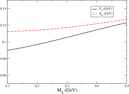
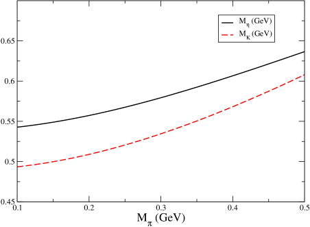
Figure 1: $M_{\pi}$ dependence (in infinite volume) of $F_{\pi},F_{K},M_{K},M_{\eta}$. For the latter three quantities the strange quark mass has been fixed as to reproduce $M_{K}^{\mathrm{phys}}$ at $M_{\pi}\!=\!M_{\pi}^{\mathrm{phys}}$.

6.3 Results

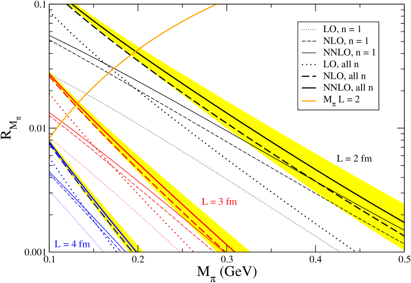
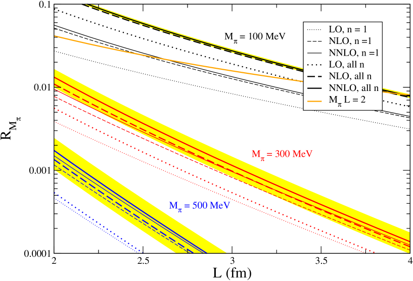
Figure 2: $R_{M_{\pi}}$ vs. $M_{\pi}$ for $L\!=\!2,3,4\,\mathrm{fm}$ (top) and vs. $L$ for $M_{\pi}\!=\!100,300,500\,\mathrm{MeV}$ (bottom). The result of the original (“$n\!=\!1$”) Lüscher formula (13) with LO/NLO/NNLO chiral input is to be compared to the resummed (“all $n$”) formula (19) which amounts to an approximate 1/2/3-loop ChPT calculation in finite volume. With NNLO input the low energy constants lead to a non-negligible error band; with NLO input the error is smaller (not shown), with LO input it is zero (see text). In the region above the $M_{\pi}L\!=\!2$ line one is not safely in the $p$-regime and our results should not be trusted.

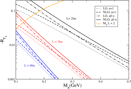
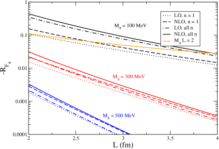
Figure 3: $-R_{F_{\pi}}$ vs. $M_{\pi}$ for $L\!=\!2,3,4\,\mathrm{fm}$ (left) and vs. $L$ for $M_{\pi}\!=\!100,300,500\,\mathrm{MeV}$ (right).

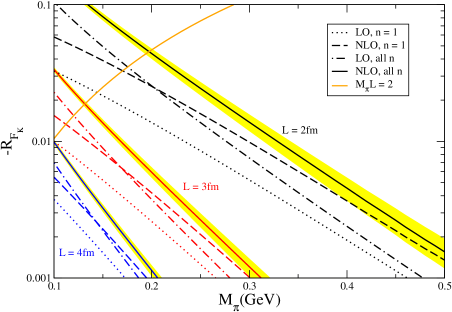
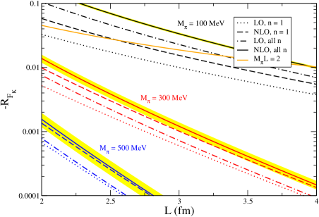
Figure 4: $-R_{F_{K}}$ vs. $M_{\pi}$ for $L\!=\!2,3,4\,\mathrm{fm}$ (left) and vs. $L$ for $M_{\pi}\!=\!100,300,500\,\mathrm{MeV}$ (right).

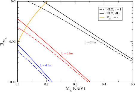
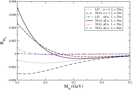
Figure 5: $R_{M_{K}}$ (left) and $R_{M_{\eta}}$ (right) vs. $M_{\pi}$ for $L\!=\!2,3,4\,\mathrm{fm}$.

We plot our results for $R_{M_{\pi}}$ in Fig. 2, both for $L\!=\!2,3,4\,\mathrm{fm}$ as a function of $M_{\pi}$ (top) and for $M_{\pi}\!=\!100,300,500\,\mathrm{MeV}$ as a function of $L$ (bottom). The result of the original (“$n\!=\!1$”) Lüscher formula (13) with LO/NLO/NNLO chiral input is shown with a thin dotted/dashed/full line, respectively. The resummed (“all $n$”) formula (19) with LO/NLO/NNLO chiral input is given with a thick dotted/dashed/full line, respectively. With NLO or NNLO input the pertinent low energy constants lead to a non-negligible error band, except for $R_{F_{\pi}}$ where the error with NLO input is of the order of the thickness of the line, with LO input it is zero. This is a consequence of our choice to disregard any uncertainty in the expansion parameter (here $\xi_{\pi}$), as discussed in the previous subsection. The area which corresponds – in the resummed scenario with NNLO input – to a situation with $M_{\pi}L\!\leq\!2$ should be disregarded, since there is no reason to hope that the resummed Lüscher formula would still capture the numerically dominating terms in a complete “ChPT in finite volume” formula to the corresponding order in the $p$-counting.

Fig. 3 contains our data for $-R_{F_{\pi}}$. They are organized in the same manner as in the previous figure, though only LO and NLO input is used, since the pertinent matrix element is known only to 1-loop order, as discussed in Sect. 4.

Finally, Figs. 4-5 contain the same information for $F_{K},M_{K},M_{\eta}$. In all these cases the asymptotic formulae with and without resummation may be compared, and the effect of going from LO to NLO input may be assessed.

$R_{M_{\pi}}$	$1.6\,\mathrm{fm}$	$1.8\,\mathrm{fm}$	$2.0\,\mathrm{fm}$	$2.2\,\mathrm{fm}$	$2.4\,\mathrm{fm}$	$2.6\,\mathrm{fm}$	$2.8\,\mathrm{fm}$	$3.0\,\mathrm{fm}$
$140\,\mathrm{MeV}$	.2099(127)	0.1292(82)	0.0830(55)	0.0552(38)	0.0377(27)	0.0264(19)	0.0188(14)	0.0136(10)
$160\,\mathrm{MeV}$	.1687(130)	0.1023(83)	0.0647(55)	0.0424(37)	0.0285(26)	0.0196(18)	0.0138(13)	0.0098(10)
$180\,\mathrm{MeV}$	.1366(130)	0.0817(82)	0.0509(53)	0.0328(35)	0.0217(24)	0.0147(17)	0.0102(12)	0.0071(09)
$200\,\mathrm{MeV}$	.1113(127)	0.0656(79)	0.0403(50)	0.0256(33)	0.0167(22)	0.0111(15)	0.0076(11)	0.0052(08)
$220\,\mathrm{MeV}$	.0912(123)	0.0529(75)	0.0320(47)	0.0200(31)	0.0129(20)	0.0084(14)	0.0056(09)	0.0038(06)
$240\,\mathrm{MeV}$	.0749(117)	0.0429(70)	0.0256(43)	0.0157(28)	0.0099(18)	0.0064(12)	0.0042(08)	0.0028(05)
$260\,\mathrm{MeV}$	.0618(110)	0.0349(65)	0.0205(39)	0.0124(25)	0.0077(16)	0.0049(10)	0.0032(07)	0.0021(05)
$280\,\mathrm{MeV}$	.0511(102)	0.0284(59)	0.0164(35)	0.0098(22)	0.0060(14)	0.0038(09)	0.0024(06)	0.0015(04)
$300\,\mathrm{MeV}$	0.0423(93)	0.0232(53)	0.0132(31)	0.0078(19)	0.0047(12)	0.0029(07)	0.0018(05)	0.0011(03)
$320\,\mathrm{MeV}$	0.0352(85)	0.0190(48)	0.0107(28)	0.0062(16)	0.0037(10)	0.0022(06)	0.0014(04)	0.0009(02)
$340\,\mathrm{MeV}$	0.0293(77)	0.0156(42)	0.0086(24)	0.0049(14)	0.0029(08)	0.0017(05)	0.0010(03)	0.0006(02)
$360\,\mathrm{MeV}$	0.0245(69)	0.0129(37)	0.0070(21)	0.0039(12)	0.0023(07)	0.0013(04)	0.0008(03)	0.0005(02)
$380\,\mathrm{MeV}$	0.0205(62)	0.0106(33)	0.0057(18)	0.0031(10)	0.0018(06)	0.0010(03)	0.0006(02)	0.0004(01)
$400\,\mathrm{MeV}$	0.0172(55)	0.0088(29)	0.0046(15)	0.0025(09)	0.0014(05)	0.0008(03)	0.0005(02)	0.0003(01)
$420\,\mathrm{MeV}$	0.0145(49)	0.0073(25)	0.0038(13)	0.0020(07)	0.0011(04)	0.0006(02)	0.0003(01)	0.0002(01)
$440\,\mathrm{MeV}$	0.0123(43)	0.0061(22)	0.0031(11)	0.0016(06)	0.0009(03)	0.0005(02)	0.0003(01)	0.0001(01)
$460\,\mathrm{MeV}$	0.0104(38)	0.0051(19)	0.0025(10)	0.0013(05)	0.0007(03)	0.0004(01)	0.0002(01)	0.0001(00)
$480\,\mathrm{MeV}$	0.0088(33)	0.0042(16)	0.0021(08)	0.0011(04)	0.0006(02)	0.0003(01)	0.0002(01)	0.0001(00)
$500\,\mathrm{MeV}$	0.0076(29)	0.0036(14)	0.0017(07)	0.0009(03)	0.0004(02)	0.0002(01)	0.0001(00)	0.0001(00)

Table 3: $R_{M_{\pi}}$ via the resummed Lüscher formula (22) with NNLO chiral input for $\mathcal{F}_{\pi}(\tilde{\nu})$, representing an approximate 3-loop result. The error includes the uncertainty of the $\bar{\ell}_{i}$ and the $O(p^{6})$ low energy constants, but no systematics. Entries with $M_{\pi}L\!<\!2$ are unlikely to really capture the physical finite size effect, and the first two columns are somewhat on the short side with respect to the condition (4).

$-R_{F_{\pi}}$	$1.6\,\mathrm{fm}$	$1.8\,\mathrm{fm}$	$2.0\,\mathrm{fm}$	$2.2\,\mathrm{fm}$	$2.4\,\mathrm{fm}$	$2.6\,\mathrm{fm}$	$2.8\,\mathrm{fm}$	$3.0\,\mathrm{fm}$
$140\,\mathrm{MeV}$	0.5844(43)	0.3683(24)	0.2414(14)	0.1633(09)	0.1134(06)	0.0804(04)	0.0581(03)	0.0426(02)
$160\,\mathrm{MeV}$	0.4551(36)	0.2828(20)	0.1827(12)	0.1218(07)	0.0833(05)	0.0581(03)	0.0413(02)	0.0298(02)
$180\,\mathrm{MeV}$	0.3580(30)	0.2194(17)	0.1397(10)	0.0917(06)	0.0618(04)	0.0424(03)	0.0297(02)	0.0211(01)
$200\,\mathrm{MeV}$	0.2840(25)	0.1715(14)	0.1076(08)	0.0696(05)	0.0461(03)	0.0312(02)	0.0215(02)	0.0150(01)
$220\,\mathrm{MeV}$	0.2267(22)	0.1350(12)	0.0834(07)	0.0531(05)	0.0347(03)	0.0231(02)	0.0156(01)	0.0107(01)
$240\,\mathrm{MeV}$	0.1820(19)	0.1068(11)	0.0650(06)	0.0408(04)	0.0262(03)	0.0171(02)	0.0114(01)	0.0077(01)
$260\,\mathrm{MeV}$	0.1467(16)	0.0848(09)	0.0509(05)	0.0314(03)	0.0198(02)	0.0128(01)	0.0084(01)	0.0056(01)
$280\,\mathrm{MeV}$	0.1188(14)	0.0677(08)	0.0399(05)	0.0243(03)	0.0151(02)	0.0095(01)	0.0061(01)	0.0040(01)
$300\,\mathrm{MeV}$	0.0965(13)	0.0541(07)	0.0315(04)	0.0188(03)	0.0115(02)	0.0072(01)	0.0045(01)	0.0029(00)
$320\,\mathrm{MeV}$	0.0786(11)	0.0434(06)	0.0249(04)	0.0146(02)	0.0088(01)	0.0054(01)	0.0033(01)	0.0021(00)
$340\,\mathrm{MeV}$	0.0642(10)	0.0350(05)	0.0197(03)	0.0114(02)	0.0067(01)	0.0040(01)	0.0025(00)	0.0015(00)
$360\,\mathrm{MeV}$	0.0527(09)	0.0282(05)	0.0156(03)	0.0089(02)	0.0052(01)	0.0031(01)	0.0018(00)	0.0011(00)
$380\,\mathrm{MeV}$	0.0433(08)	0.0228(04)	0.0124(02)	0.0070(01)	0.0040(01)	0.0023(00)	0.0014(00)	0.0008(00)
$400\,\mathrm{MeV}$	0.0356(07)	0.0185(04)	0.0099(02)	0.0055(01)	0.0031(01)	0.0017(00)	0.0010(00)	0.0006(00)
$420\,\mathrm{MeV}$	0.0294(06)	0.0150(03)	0.0079(02)	0.0043(01)	0.0024(01)	0.0013(00)	0.0008(00)	0.0004(00)
$440\,\mathrm{MeV}$	0.0244(05)	0.0122(03)	0.0063(01)	0.0034(01)	0.0018(00)	0.0010(00)	0.0006(00)	0.0003(00)
$460\,\mathrm{MeV}$	0.0202(05)	0.0100(02)	0.0051(01)	0.0027(01)	0.0014(00)	0.0008(00)	0.0004(00)	0.0002(00)
$480\,\mathrm{MeV}$	0.0169(04)	0.0082(02)	0.0041(01)	0.0021(01)	0.0011(00)	0.0006(00)	0.0003(00)	0.0002(00)
$500\,\mathrm{MeV}$	0.0141(04)	0.0067(02)	0.0033(01)	0.0017(00)	0.0009(00)	0.0004(00)	0.0002(00)	0.0001(00)

Table 4: $-R_{F_{\pi}}$ via the resummed Lüscher formula (23) with NLO chiral input for $\mathcal{N}_{\pi}(\tilde{\nu})$, representing an approximate 2-loop result. The error includes the uncertainty of the $\bar{\ell}_{i}$, but no systematics. Entries with $M_{\pi}L\!<\!2$ are unlikely to really capture the physical finite size effect, and the first two columns are somewhat on the short side with respect to the condition (4).

The main message to be extracted from Figs. 2-5 is that the relative finite volume shift vanishes indeed in proportion to $e^{-M_{\pi}L}$; in the logarithmic representation one has an almost linear fall-off pattern, and higher orders mainly affect the prefactor. The second point concerns the relative importance of higher orders in the chiral counting versus higher exponentials. For small pion masses (say $100\,\mathrm{MeV}$) resumming (i.e. higher exponentials) prove vital, while for large pion masses (say $500\,\mathrm{MeV}$) higher loop orders prove more relevant (though the effect is small in that regime). As has been discussed in Ref. [15] a large shift in $R_{M_{P}}$, when moving from LO to NLO input, does not necessarily signal a bad chiral convergence behavior, since the cut in the underlying $\mathcal{F}_{P}$ amplitude starts only at the NLO level. Unfortunately, the effect due to an upgrade to NNLO input can only be checked in the case of $R_{M_{\pi}}$, since only there the pertinent amplitude is known. Nonetheless, we believe that the regime in the $(M_{\pi},L)$ plane that leads to a nice convergence behavior in $R_{M_{\pi}}$ is indicative of the regime where the resummed formulae for $R_{F_{\pi}},R_{M_{K}},R_{F_{K}},R_{M_{\eta}}$ with NLO input yield a trustworthy result.

For $R_{M_{\pi}}$ and $R_{F_{\pi}}$ the numerical results to the highest loop order available (equivalent to an approximate 3-loop and 2-loop calculation in ChPT) have been collected in Tabs. 4 and 4, respectively. From the general discussion it is clear that the logarithms of the numbers in these tables may be interpolated with a low-order polynomial.

7 Two types of applications

We finish with a discussion of two prototype applications of our formulae. The first one is a “forward-type” application, in which our formulae are used to control a systematic error in a lattice calculation. The second one concerns a “backward-type” application, where one tries to determine QCD low energy constants from explicitly measuring finite-volume effects.

7.1 Finite volume effects and Marciano’s determination of $V_{us}$

An example of how an analytic finite volume calculation may help to control a systematic error is the following. Marciano pointed out that, modulo radiative corrections, the ratio $\frac{V_{us}}{V_{ud}}\frac{F_{K}}{F_{\pi}}$ is fixed by the ratio of branching ratios for $K_{\ell 2}$ and $\pi_{\ell 2}$ decays. Taking into account radiative corrections, he obtained the following relation [35]

$${|V_{us}|^{2}\over|V_{ud}|^{2}}{F_{K}^{2}\over F_{\pi}^{2}}=0.07602(23)(27)$$ (66)

where the errors represent the experimental and radiative correction uncertainties. He then suggested to combine the value for $V_{ud}$ obtained from superallowed nuclear beta decays with a value for $F_{K}/F_{\pi}$ from lattice simulations. We stress that the necessary accuracy to make an impact on the determination of $V_{us}$ is at the level of 1% or better, and indeed, both the determination of $V_{ud}$ as well as the ratio of branching ratios are known to well below 1%. This means that any improvement in the lattice calculation of $F_{K}/F_{\pi}$ will be immediately reflected in the value of $V_{us}$. In particular, being able to control systematic effects to well below 1% is of crucial importance.

With our results for $R_{F_{\pi}}$ and $R_{F_{K}}$ it is straightforward to calculate the finite-volume shift of the latter ratio

$${F_{K}(L)\over F_{\pi}(L)}={F_{K}\over F_{\pi}}\;\Big{\{}1+R_{F_{K}}-R_{F_{\pi}}+\mathcal{O}(R_{F}^{2})\Big{\}}$$ (67)

and thus to compare the magnitude of this effect to the typical size of the statistical error. A plot of the finite volume effect for the ratio of decay constants as a function of the pion mass and for a few volume sizes is provided in Fig. 6.

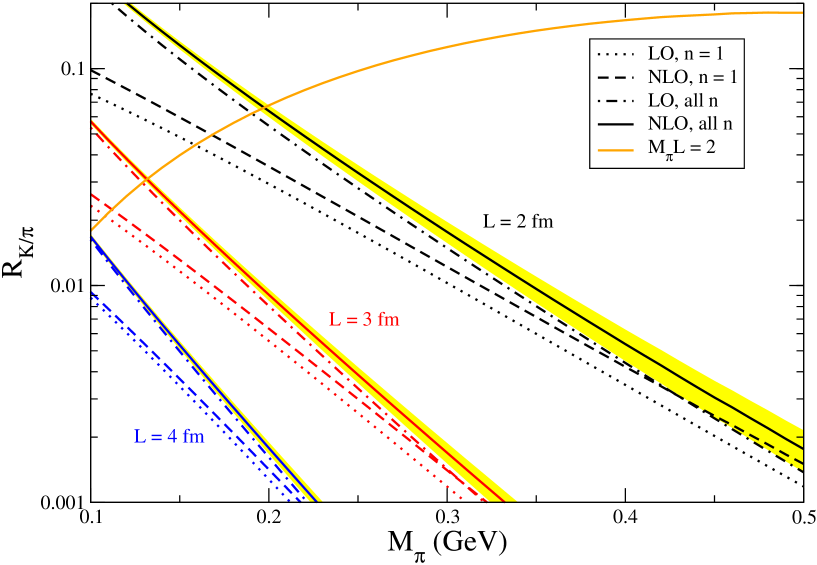
Figure 6: The relative finite volume effect $(F_{K}(L)F_{\pi})/(F_{\pi}(L)F_{K})-1$ vs. $M_{\pi}$ for $L\!=\!2,3,4\,\mathrm{fm}$. Above the $M_{\pi}L\!=\!2$ line one is not safely in the $p$-regime and our results should not be trusted.

In his analysis Marciano uses the MILC Collaboration result $F_{K}/F_{\pi}=1.201(8)(15)$ [36, 37]. Among the various data sets they have, those with the smallest $M_{\pi}L$ and thus most likely to be affected by sizeable finite volume corrections, have $M_{\pi}(L)\!\simeq\!311\,\mathrm{MeV}$, $L\!\simeq\!2.4\,\mathrm{fm}$ and $M_{\pi}(L)\!\simeq\!262\,\mathrm{MeV}$, $L\!\simeq\!2.89\,\mathrm{fm}$. Using (67) we find that with the parameters of the first set $F_{K}(L)/F_{\pi}(L)$ in the continuum deviates from the infinite volume result by $0.0099-0.0038=0.61$%, while the corresponding estimate for the second set reads $0.0067-0.0025=0.42$%. A systematic effect of half a percent needs to be taken into account in a high precision study, and from Fig. 6 one sees that other ($M_{\pi},L$) pairs to reach that level would be ($410\,\mathrm{MeV},2\,\mathrm{fm}$), ($230\,\mathrm{MeV},3\,\mathrm{fm}$) and ($150\,\mathrm{MeV},4\,\mathrm{fm}$).

We stress that the numerical example just discussed is for illustrative purposes only, because we do not know whether our formulae can be applied to the MILC Collaboration data. Lattice QCD with staggered fermions and $N_{\!f\,}\!=\!2$ or $N_{\!f\,}\!=\!2\!+\!1$ violates flavour (or taste) symmetry and low energy unitarity, properties our analysis relies on. Under the assumption that these effects disappear in the continuum limit , the finite volume shift of an observable like $F_{\pi}/F_{K}$ can be calculated in staggered chiral perturbation theory (this is what the MILC Collaboration does [39]), but one cannot enjoy the benefits of the Lüscher formula. We stress that no such conceptual issues arise with dynamical Wilson-type fermions. In such a case our continuum formulae can be directly applied to the data at finite lattice spacing with cut-off effects bringing only mild (i.e. numerically irrelevant) modifications as discussed in App. B.

7.2 Low energy constants from finite volume effects

In the present section we discuss whether one can use these finite volume effects to obtain information on the low energy constants from lattice calculations. At first sight this seems unpractical, because these effects are quite small and decay exponentially with $M_{\pi}L$. This means that, roughly speaking, if one wishes to obtain information on (a combination of) low energy constants to a certain accuracy, one has to calculate the corresponding particle mass or decay constant to an accuracy which is about two orders of magnitude higher, and this is a challenge. The asymptotic formulae provide a connection between finite volume effects on two-point functions and (infinite volume) four-point functions, and thus give us access to low energy constants that appear as local contributions to four-point functions. The question is then what alternative ways one has to measure these constants on the lattice. It is well known that the $P\pi$ scattering amplitudes which govern the finite volume corrections to the mass of the $P$ particle can be obtained more directly by evaluating the finite volume dependence of the energy of the state of two particles $P$ and $\pi$ enclosed in a box [40]. This method is more direct because the effect is suppressed only by powers of the volume rather than exponentially. Still, such a calculation is very difficult, also because the typical volume needed is quite large.

There is another important difference between the two methods. As we have seen in Sect. 5.2 the analytic representation of the finite volume effects is enormously simplified if one Taylor expands the amplitudes in the Lüscher-type formulae. Here, two terms in the Taylor expansion are enough for a very accurate representation. The extraction of the low energy constants from these effects can be viewed as a two-step process: one first determines the values of the first two Taylor coefficients of the amplitudes at $\nu=0$, and then from these the low energy constants. The chiral representation enters only in this second step. Analogously, if one uses the method with two particles in a box, one first determines the scattering lengths, and then extracts from these the relevant low energy constants. As discussed in [30], the scattering lengths have a badly converging chiral expansion, such that only at very small quark masses one would be able to reliably extract the low energy constants. This happens because one is evaluating the amplitude on top of the threshold singularity. At $\nu=0$, below threshold and away from any other singularity, the amplitude displays a better convergence. For all these reasons we believe it is worthwhile to explore this alternative route.

The quantities which are worth considering for our scope are $M_{\pi}$, $F_{\pi}$ and $F_{K}$. We write the relative finite volume shifts in the form

$$R_{X}=R_{X}^{0}+c_{X}\Big{(}\beta^{0}L_{X}^{0}+\beta^{2}L_{X}^{2}\Big{)}$$ (68)

where $R_{X}^{0}$ represents contributions independent of the low energy constants, and the coefficients $c_{X}$ are defined as

$$c_{M_{\pi}}=-\xi_{\pi}^{2}\;,\quad c_{F_{\pi}}=\xi_{\pi}^{2}\;,\quad c_{F_{K}}=12N\frac{F_{\pi}}{F_{K}}\xi_{\pi}\xi_{K}\;\;.$$ (69)

The functions $\beta^{0,2}$ are series of Bessel functions and depend on $\lambda_{\pi}$ only

$$\beta^{0,2}=\sum_{n=1}^{\infty}{m(n)\over\sqrt{n}\lambda_{\pi}}B^{0,2}(\sqrt{n}\lambda_{\pi})\;\;.$$ (70)

They are plotted in Fig. 7.

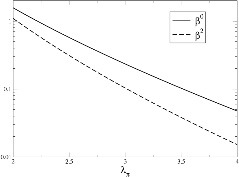
Figure 7: The functions $\beta^{0,2}$.

The $L_{X}^{0,2}$ are the combinations of low energy constants that appear in each of the quantities to next-to-leading order. In particular we read off from the formulae (22,23) and (47,52,55)

$$\begin{array}[]{llllll}L_{M_{\pi}}^{0}&=&2(\bar{\ell}_{1}+{2\over 3}\bar{\ell}_{2})-{5\over 4}\bar{\ell}_{3}-\bar{\ell}_{4}&L_{M_{\pi}}^{2}&=&-{4\over 3}(\bar{\ell}_{1}+4\bar{\ell}_{2})\\[4.2679pt] L_{F_{\pi}}^{0}&=&2(\bar{\ell}_{1}+{2\over 3}\bar{\ell}_{2})-3\bar{\ell}_{4}&L_{F_{\pi}}^{2}&=&-{8\over 3}(\bar{\ell}_{1}+4\bar{\ell}_{2})\\[4.2679pt] L_{F_{K}}^{0}&=&x_{\pi K}(4L_{1}^{\mathrm{r}}+L_{3}^{\mathrm{r}}-2L_{4}^{\mathrm{r}})-{1\over 4}(1+x_{\pi K})L_{5}^{\mathrm{r}}&L_{F_{K}}^{2}&=&-2x_{\pi K}(4L_{2}^{\mathrm{r}}+L_{3}^{\mathrm{r}})\;.\end{array}$$

It is interesting that both $M_{\pi}$ and $F_{\pi}$ are sensitive to the same combination of $\bar{\ell}_{1}$ and $\bar{\ell}_{2}$ (note that $\bar{\ell}_{3}$ and $\bar{\ell}_{4}$ can be pinned down directly from the quark mass dependence of $M_{\pi}$ and $F_{\pi}$, respectively). This means that one can determine the low energy constants which fix the $\pi\pi$ scattering amplitude also from the finite volume effects for $F_{\pi}$ where the $\pi\pi$ scattering amplitude does not appear. One should remark that the sensitivity to the combination $(\bar{\ell}_{1}+{2\over 3}\bar{\ell}_{2})$ is the same, whereas $F_{\pi}$ is a factor two more sensitive to the combination $(\bar{\ell}_{1}+4\bar{\ell}_{2})$.

To discuss the numerics we fix $M_{\pi}\!=\!300$ MeV and $L\!=\!2$ fm. In this setting $\beta^{0}\!=\!0.22$, $\beta^{2}\!=\!0.10$, and $c_{M_{\pi}}=-0.0026$, $c_{F_{\pi}}=0.0026$. A change of one unit in the combination $(\bar{\ell}_{1}+{2\over 3}\bar{\ell}_{2})$ then generates a shift of about 0.12% in both $M_{\pi}(L)$ and $F_{\pi}(L)$. According to Tab. 2 this linear combination is known from phenomenology to be

$$(\bar{\ell}_{1}+{2\over 3}\bar{\ell}_{2})_{|_{M_{\pi}=300\mathrm{MeV}}}=-0.1\pm 0.6\;\;.$$ (71)

On the other hand a change of one unit in $(\bar{\ell}_{1}+4\bar{\ell}_{2})$ modifies $F_{\pi}(L)$ by 0.07% and $M_{\pi}(L)$ by half that much. This linear combination, however, is known to be larger from phenomenology

$$(\bar{\ell}_{1}+4\bar{\ell}_{2})_{|_{M_{\pi}=300\mathrm{MeV}}}=9.1\pm 0.5\;\;.$$ (72)

This numerical example indicates that in order to get a reasonable account on these combinations of low energy constants, one would have to control the pion mass and decay constant for $M_{\pi}\!=\!300\,\mathrm{MeV}$ and $L\!=\!2\,\mathrm{fm}$ to less than 1 permille, which is a real challenge.

An alternative way, as already mentioned, would be to calculate the $\pi\pi$ $S$-wave $I\!=\!2$ scattering lengths via Lüscher’s method [40]. There are some results with dynamical fermions for this quantity [41], but not yet precise enough and for low enough pion masses that would allow an extraction of the relevant low energy constant. We mention in passing that both $a^{2}_{0}$ and $a^{0}_{0}$ (the latter is even more difficult to calculate on the lattice, and shows a very badly converging chiral expansion [30]) are sensitive to the combination $\bar{\ell}_{1}+2\bar{\ell}_{2}$, and therefore provide complementary information to the one that would be obtained from the finite volume effects we have discussed here.

The numerics for the $F_{K}$ case is similar. Again, in order to get a sensitivity comparable to the one which characterizes the phenomenological determination (notice that the $L_{i}^{\mathrm{r}}$ constants are usually given in units of $10^{-3}$) one would have to calculate $F_{K}$ to the permille accuracy.

8 Conclusions

In this paper we have carefully analyzed the finite volume effects on masses and decay constants of the lightest pseudoscalar mesons. The theoretical framework in which we carry out this analysis has been set up long ago by Gasser and Leutwyler [5] and by Lüscher [13]. The former two discussed how ChPT can be adapted to the case of a finite box and then be used to calculate finite volume effects. The latter author derived a formula valid for large volumes which expresses the finite volume effects in terms of an integral over a physical scattering amplitude. This formula does not rely on ChPT, but for QCD is best used in combination with ChPT: this is the tool to provide a representation of the necessary scattering amplitude as a function of quark masses. More recently a formula à la Lüscher for decay constants has been derived by two of us [16]. In the present paper we have proposed a resummation of the asymptotic formulae as the best tool to study finite volume effects for masses and decay constants. The resummation is a simple, “kinematical” extension of the asymptotic formulae, which however does improve the algebraic accuracy of the formula. Used in combination with the chiral representation for the scattering amplitude in the integral it yields an accurate determination of finite volume effects.

Our numerical results show that decay constants and masses of the pseudoscalars are in general little affected by the finite spatial size of the box (as soon as the box is large enough that ChPT can be applied, $L\!\geq\!2\,\mathrm{fm}$). For the smallest acceptable values of $M_{\pi}L$ (in the $p$-regime, in which we are working, this quantity has to be larger than one) they are typically of the order of a few percent for $M_{\pi}$, $F_{\pi}$ and $F_{K}$. We have seen that in the $p$-regime $M_{K}$ and $M_{\eta}$ are practically insensitive to the box size. Independently of the exact size of these corrections we could always check the convergence of the chiral expansion and conclude that these finite volume effects are under good theoretical control. This means that if one’s goal is to calculate masses or decay constants one can use the results of this paper to choose the volume in order to minimize the calculational costs. For example, by using a box of $2\,\mathrm{fm}$ size (which our results show to be sufficiently large) and explicitly correcting for the finite volume effects one can save computational costs with respect to a $2.5\,\mathrm{fm}$ size box which (for pion masses of about 300 MeV or larger) gives finite volume effects below 1%. The gain in CPU time that comes from such a reduction of the volume by almost a factor 2 can be used more fruitfully by pushing towards smaller lattice spacings and/or lighter quark masses.

Since our results are theory predictions, an explicit check by lattice calculations would of course be very welcome, but it would require a high precision. Once this level of accuracy will be reached, our formulae will become particularly useful. First, in order to correct for these effects in all applications which require a high precision, like the evaluation of the $F_{K}/F_{\pi}$ ratio which, as suggested by Marciano [35], leads to a determination of $V_{us}$ [39]. Second, if one wants to use these finite size effects as a means to determine low energy constants on the lattice. As we have discussed, despite the fact that these effects are exponentially suppressed and numerically quite small in all practical situations, they do offer the advantage of involving in two-point functions low energy constants which, otherwise, appear only in four-point functions. The latter are quantities which are very difficult to determine directly on the lattice, and it may therefore turn out to be easier to see them indirectly, through a small correction to an “easy” quantity like the pion mass or decay constant.

Acknowledgments

We are indebted to Peter Hasenfratz, Heiri Leutwyler and Rainer Sommer for useful discussions and/or comments on the manuscript. This work has been supported by the Schweizerischer Nationalfonds and partly by the EU “Euridice” program under code HPRN-CT2002-00311.

Appendix A The integrals $S_{M_{P}}^{(n)}$ and $S_{F_{P}}^{(n)}$

In this appendix we give explicitly the contributions from loop functions to the finite volume effects. These have been introduced and defined in Sect. 5. The expression for the pion related integrals have already been given in [15, 16]. We give them here for convenience:

$$S^{(4)}_{M_{\pi}} = {13\over 3}R_{0}^{0}-{16\over 3}R_{0}^{1}-{40\over 3}R_{0}^{2}$$

$$S_{M_{\pi}}^{(6)} = R_{0}^{0}\Big{(}{817\over 27}+{80\over 9}\bar{\ell}_{2}-5\bar{\ell}_{3}+{52\over 3}\bar{\ell}_{4}\Big{)}-{2\over 3}R_{0}^{1}\Big{(}{313\over 9}+{40\over 3}\bar{\ell}_{2}+32\bar{\ell}_{4}\Big{)}$$

$$+ R_{0}^{2}\Big{(}{292\over 27}-8\bar{\ell}_{1}-{128\over 9}\bar{\ell}_{2}-{160\over 3}\bar{\ell}_{4}\Big{)}+{4\over 3}R_{0}^{3}\Big{(}-{47\over 9}+4\bar{\ell}_{1}-4\bar{\ell}_{2}\Big{)}$$

$$+ {1\over 9}R_{1}^{0}\Big{(}1-{\pi^{2}\over 2}\Big{)}+{1\over 9}R_{1}^{1}\Big{(}128-{\pi^{2}\over 8}\Big{)}-{1\over 3}R_{1}^{2}\Big{(}{100\over 3}+{\pi^{2}\over 8}\Big{)}$$

$$+ {1\over 6}R_{2}^{0}\Big{(}7-{\pi^{2}\over 3}\Big{)}+{1\over 9}R_{2}^{1}\Big{(}16+{7\pi^{2}\over 8}\Big{)}+{\pi^{2}\over 24}R_{2}^{2}$$

$$- {46\over 9}R_{3}^{0}-{32\over 9}R_{3}^{1}-{32\over 3}R_{3}^{2}+{40\over 3}\Big{(}R_{4}^{0}+R_{4}^{1}\Big{)}$$

$$S^{(4)}_{F_{\pi}} = \frac{4}{3}\Big{(}R_{0}^{0}-R_{0}^{1}-10R_{0}^{2}\Big{)}-{13\over 6}R_{0}^{0\prime}+{8\over 3}R_{0}^{1\prime}+{20\over 3}R_{0}^{2\prime}$$ (73)

where the integrals $R_{i}^{k}$ are defined as

$$R_{0}^{k(\prime)}\! \!\equiv\! \!R_{0}^{k(\prime)}(\sqrt{n}\lambda_{\pi})=\left\{{\mathrm{Re}\atop\mathrm{Im}}\right.\int_{-\infty}^{\infty}\!d\tilde{y}\;\tilde{y}^{k}\,e^{-\sqrt{n(1+\tilde{y}^{2})}\,\lambda_{\pi}}\,g^{(\prime)}(2+2\mathrm{i}\tilde{y})\qquad\;\;\;\;\mathrm{for}\;\left\{{k\;\mathrm{even}\atop k\;\mathrm{odd}}\right.$$ (74)

$$R_{i}^{k}\;\;\! \!\equiv\! \!\;\;R_{i}^{k\;}(\sqrt{n}\lambda_{\pi})=\left\{{\mathrm{Re}\atop\mathrm{Im}}\right.\int_{-\infty}^{\infty}\!d\tilde{y}\;\tilde{y}^{k}\,e^{-\sqrt{n(1+\tilde{y}^{2})}\,\lambda_{\pi}}\,N^{2}\,K_{i}^{\pi\pi}(2+2\mathrm{i}\tilde{y})\;\;\;\;\mathrm{for}\;\left\{{k\;\mathrm{even}\atop k\;\mathrm{odd}}\right.$$ (75)

with $g^{(\prime)}$ defined in (58) and

$$K_{1}^{\pi\pi}(x) = {1\over N^{2}\sigma^{2}}\Big{[}g(x)-2\Big{]}^{2}$$

$$K_{2}^{\pi\pi}(x) = {1\over N^{2}}\Big{[}g(x)^{2}-4g(x)\Big{]}$$

$$K_{3}^{\pi\pi}(x) = {1\over 2N^{2}\sigma^{4}x}\Big{[}2g(x)^{3}-12g(x)^{2}+24g(x)+2\pi^{2}\sigma^{2}g(x)-16-\pi^{2}\sigma^{2}x\Big{]}$$

$$K_{4}^{\pi\pi}(x) = {1\over\sigma^{2}x}\Big{[}K_{0}^{\pi\pi}(x)+{1\over 2}K_{1}^{\pi\pi}(x)+{1\over 3}K_{3}^{\pi\pi}(x)+{(\pi^{2}-6)x\over 12N^{2}}\Big{]}$$ (76)

with $\sigma=\sqrt{1-4/x}$. As seen in (74), in $S^{(4)}_{F_{\pi}}$ integrals over the derivative of the function $g$ appear. This is a consequence of the subtraction procedure (33). In the practical implementation one writes $s_{1}=2M_{\pi}^{2}-2\nu M_{\pi}+(Q^{2}-M_{\pi}^{2})/2-s_{3}/2$ and $s_{2}=2M_{\pi}^{2}+2\nu M_{\pi}+(Q^{2}-M_{\pi}^{2})/2-s_{3}/2$ to trade $s_{1},s_{2}$ for $Q^{2}-M_{\pi}^{2},\nu$ and expands $A_{\pi}^{I=0}$ consistently in these new variables. For instance in $F_{0}$ one substitutes $\bar{J}(s_{1})\to\bar{J}(2M_{\pi}^{2}-2\nu M_{\pi})+\bar{J}^{\prime}(2M_{\pi}^{2}-2\nu M_{\pi})[Q^{2}-M_{\pi}^{2}-s_{3}]/2$.

The loop integrals for kaon and eta finite volume effects read:

$$S_{M_{K}}^{(4)} = 3\bigg{\{}\frac{3}{32}(1+x_{\pi K})^{2}S^{0,1}_{K\pi}-\frac{5}{8}(1+x_{\pi K})S^{1,1}_{K\pi}-\frac{19}{8}S^{2,1}_{K\pi}-\frac{3}{16}(1-x_{\pi K}^{2})S^{0,3}_{K\pi}$$

$$+ \frac{13}{8}(1-x_{\pi K})S^{1,3}_{K\pi}-\frac{3}{2}\left(x_{\pi K}S^{0,5}_{K\pi}+S^{2,5}_{K\pi}\right)+\frac{1}{96}(1+x_{\pi K})^{2}S^{0,1}_{\eta K}$$

$$- \frac{1}{8}(1+x_{\pi K})S^{1,1}_{\eta K}-\frac{3}{8}S^{2,1}_{\eta K}+\frac{1}{16}(1+x_{\pi K})(3x_{\eta K}+2x_{\pi K}-5)S^{0,3}_{\eta K}$$

$$+ \frac{3}{8}(1-2x_{\pi K}+x_{\eta K})S^{1,3}_{\eta K}-\frac{3}{2}\left(x_{\pi K}S^{0,5}_{\eta K}+S^{2,5}_{\eta K}\right)\bigg{\}}$$

$$S_{F_{K}}^{(4)} = \frac{M_{K}}{M_{\pi}}\bigg{[}-\frac{15}{16}(1+x_{\pi K})S^{1,1}_{K\pi}-\frac{57}{8}S^{2,1}_{K\pi}-\frac{9}{64}(1+x_{\pi K})^{2}S^{0,2}_{K\pi}$$

$$+ \frac{15}{16}(1+x_{\pi K})S^{1,2}_{K\pi}+\frac{57}{16}S^{2,2}_{K\pi}+\frac{9}{32}(1-5x_{\pi K})S^{0,3}_{K\pi}+\left(6-\frac{15}{8}x_{\pi K}\right)S^{1,3}_{K\pi}$$

$$+ \frac{15}{4}S^{2,3}_{K\pi}+\frac{9}{32}(1-x_{\pi K}^{2})S^{0,4}_{K\pi}-\frac{39}{16}(1-x_{\pi K})S^{1,4}_{K\pi}$$

$$- \frac{9}{4}\left(x_{\pi K}S^{0,5}_{K\pi}+2S^{2,5}_{K\pi}-x_{\pi K}S^{0,6}_{K\pi}-S^{2,6}_{K\pi}\right)$$

$$- \frac{3}{16}(1+x_{\pi K})S^{1,1}_{\eta K}-\frac{9}{8}S^{2,1}_{\eta K}-\frac{1}{64}(1+x_{\pi K})^{2}S^{0,2}_{\eta K}+\frac{3}{16}(1+x_{\pi K})S^{1,2}_{\eta K}$$

$$+ \frac{9}{16}S^{2,2}_{\eta K}+\left(\frac{27}{32}(x_{\eta K}-1)-\frac{3}{16}(1+x_{\pi K})\right)S^{0,3}_{\eta K}$$

$$+ \frac{3}{8}(4-2x_{\pi K}+3x_{\eta K})S^{1,3}_{\eta K}+\frac{9}{4}S^{2,3}_{\eta K}+\frac{3}{32}(5-3x_{\eta K})(1-x_{\pi K}^{2})S^{0,4}_{\eta K}$$

$$- \frac{9}{16}(1-2x_{\pi K}+x_{\eta K})S^{1,4}_{\eta K}-\frac{9}{4}\left(x_{\pi K}S^{0,5}_{\eta K}+2S^{2,5}_{\eta K}-x_{\pi K}S^{0,6}_{\eta K}-S^{2,6}_{\eta K}\right)\bigg{]}$$

$$S^{(4)}_{M_{\eta}} = x_{\pi\eta}^{2}T^{0,1}_{KK}-6x_{\pi\eta}T^{1,1}_{KK}-9T^{2,1}_{KK}+\frac{2}{3}x_{\pi\eta}^{2}T^{0,1}_{\eta\pi}$$ (77)

where we have introduced the following abbreviations

$$x_{PQ}=\frac{M_{P}^{2}}{M_{Q}^{2}}\;,\qquad\ell_{P}=\ln\left(\frac{M_{P}^{2}}{\mu^{2}}\right)\;\;.$$ (78)

The integrals $B^{2k}$ are proportional to modified Bessel functions

$$B^{2k}\equiv B^{2k}(\sqrt{n}\lambda_{\pi})=\int_{-\infty}^{\infty}\!d\tilde{y}\;\tilde{y}^{2k}\,e^{-\sqrt{n(1+\tilde{y}^{2})}\,\lambda_{\pi}}={\Gamma(k+1/2)\over\Gamma(3/2)}\Big{(}{2\over\sqrt{n}\lambda_{\pi}}\Big{)}^{k}K_{k+1}(\sqrt{n}\lambda_{\pi})$$ (79)

and the quantities $S^{k,I}_{PQ}$ and $T^{k,I}_{PQ}$ are integrals over functions $g_{PQ}^{I}$ which occur at one-loop order in the chiral expansion. They are all analytical along the integration line. The expressions $S^{k,I}_{PQ}$ and $T^{k,I}_{PQ}$ are defined as

$$S_{PQ}^{k,I} = \left\{{\mathrm{Re}\atop\mathrm{Im}}\right.Nx_{\pi K}^{(k+1)/2}\int_{-\infty}^{\infty}d\tilde{y}\;\tilde{y}^{k}\,e^{-\sqrt{n(1+\tilde{y}^{2})}\,\lambda_{\pi}}g_{PQ}^{(I)}(M_{K}^{2}+M_{\pi}^{2}+2\mathrm{i}M_{K}M_{\pi}\tilde{y})\qquad\mathrm{for}\left\{{k\;\mathrm{even}}\atop{k\;\mathrm{odd}}\right.$$

$$T_{PQ}^{k,I} = \left\{{\mathrm{Re}\atop\mathrm{Im}}\right.Nx_{\pi\eta}^{(k+1)/2}\int_{-\infty}^{\infty}d\tilde{y}\;\tilde{y}^{k}\,e^{-\sqrt{n(1+\tilde{y}^{2})}\,\lambda_{\pi}}g_{PQ}^{(I)}(\,M_{\eta}^{2}\,+M_{\pi}^{2}+2\mathrm{i}\,M_{\eta}M_{\pi}\tilde{y})\qquad\mathrm{for}\left\{{k\;\mathrm{even}}\atop{k\;\mathrm{odd}}\right.$$

with

$$\begin{array}[]{rclrcl}g_{PQ}^{(1)}(x)\!&\!=\!&\!\bar{J}_{PQ}(x)\;,&g_{PQ}^{(2)}(x)\!&\!=\!&\!M_{K}^{2}\bar{J}^{\prime}_{PQ}(x)\\ g_{PQ}^{(3)}(x)\!&\!=\!&\!K_{PQ}(x)\;,&g_{PQ}^{(4)}(x)\!&\!=\!&\!M_{K}^{2}K^{\prime}_{PQ}(x)\\ g_{PQ}^{(5)}(x)\!&\!=\!&\!\bar{M}_{PQ}(x)\;,&g_{PQ}^{(6)}(x)\!&\!=\!&\!M_{K}^{2}\bar{M}^{\prime}_{PQ}(x)\;.\end{array}$$

For completeness, we give the explicit expressions for the $g_{PQ}^{I}$ [25]. All functions can be expressed in terms of the subtracted scalar integral $\bar{J}(t)\!=\!J(t)\!-\!J(0)$ evaluated in four dimensions

$$J(t)=-\mathrm{i}\int\!\frac{d^{d}p}{(2\pi)^{d}}\;\;\frac{1}{((p+k)^{2}-M^{2})(p^{2}-m^{2})}$$ (80)

with $t=k^{2}$. The functions used in the text are then

$$\bar{J}(t) = -\frac{1}{N}\int_{0}^{1}dx~{}\ln\frac{M^{2}-tx(1-x)-\Delta x}{M^{2}-\Delta x}$$

$$= \frac{1}{2N}\left\{2+\frac{\Delta}{t}\ln\frac{m^{2}}{M^{2}}-\frac{\Sigma}{\Delta}\ln\frac{m^{2}}{M^{2}}-\frac{\sqrt{\rho}}{t}\ln\frac{(t+\sqrt{\rho})^{2}-\Delta^{2}}{(t-\sqrt{\rho})^{2}-\Delta^{2}}\right\}$$

$$\bar{J}^{\prime}(t) = -\frac{2}{N}\frac{M^{2}m^{2}}{(t-\Sigma)^{2}-\rho}\frac{1}{t^{2}}\bigg{[}2t+\Delta\ln\frac{m^{2}}{M^{2}}+\frac{t\Sigma-\Delta^{2}}{\sqrt{\rho}}\ln\frac{(t+\sqrt{\rho})^{2}-\Delta^{2}}{(t-\sqrt{\rho})^{2}-\Delta^{2}}\bigg{]}$$

$$K(t) = \frac{\Delta}{2t}\bar{J}(t)$$

$$K^{\prime}(t) = -\frac{\Delta}{2t}\left(\frac{\bar{J}(t)}{t}-\bar{J}^{\prime}(t)\right)$$

$$\bar{M}(t) = \frac{1}{12t}\left\{t-2\Sigma\right\}\bar{J}(t)+\frac{\Delta^{2}}{3t^{2}}\bar{J}(t)+\frac{1}{18N}-\frac{1}{6Nt}\left\{\Sigma+2\frac{M^{2}m^{2}}{\Delta}\ln\frac{m^{2}}{M^{2}}\right\}$$

$$\bar{M}^{\prime}(t) = \frac{1}{6t^{2}}\bigg{[}\frac{\Sigma t-4\Delta^{2}}{t}\bar{J}(t)+\frac{1}{2}(t^{2}-2t\Sigma+4\Delta^{2})\bar{J}^{\prime}(t)+\frac{1}{N}\left(\Sigma+\frac{2M^{2}m^{2}}{\Delta}\ln\frac{m^{2}}{M^{2}}\right)\bigg{]}$$ (81)

where

$$\Delta=M^{2}-m^{2}\;,\qquad\Sigma=M^{2}+m^{2}\;,\qquad\rho=\rho(t,M^{2},m^{2})=(t+\Delta)^{2}-4tM^{2}\;\;.$$ (82)

In the text these are used with subscripts

$$\bar{J}_{PQ}(t)=\bar{J}(t)~{}~{}~{}\mbox{with}~{}~{}~{}M=M_{P},m=M_{Q}~{}$$ (83)

and similarly for the other symbols. We add a remark concerning the analyticity properties of the loop functions. The asymptotic formula requires them to be evaluated for complex arguments. There is one case, where the representation of Eq.(A) does not yet provide an unambiguous analytic continuation, namely for $\bar{J}_{PQ}(M_{P}^{2}+M_{Q}^{2}+2\mathrm{i}M_{P}M_{Q}\tilde{y})$, because $\rho=-4M_{P}^{2}M_{Q}^{2}(1+\tilde{y}^{2})$. The correct analytical continuation is given by

$$\sqrt{\rho}=2\mathrm{i}M_{P}M_{Q}\omega\\$$

with $\omega=\sqrt{1+\tilde{y}^{2}}$, implying for the logarithm in Eq.(A) (for $t=M_{P}^{2}+M_{Q}^{2}+2\mathrm{i}M_{P}M_{Q}\tilde{y}$),

$$\ln\frac{(t+\sqrt{\rho})^{2}-\Delta^{2}}{(t-\sqrt{\rho})^{2}-\Delta^{2}}=\ln{\omega+\tilde{y}\over\omega-\tilde{y}}\left\{{+\mathrm{i}\pi\qquad\mathrm{for}\;{\tilde{y}<0}\atop-\mathrm{i}\pi\qquad\mathrm{for}\,{\tilde{y}>0}}\right.\;\;.$$ (84)

All loop functions are now well defined along the integration line in the asymptotic formulae.

Appendix B Cut-off effects

In this appendix we wish to discuss whether it is sufficient to calculate finite volume effects in continuum ChPT or whether cut-off effects should be taken care of when correcting actual lattice data for the effect of the finite spatial box length $L$.

Naive reasoning suggests that – because finite volume effects are due to the pion cloud around a particle and thus to pure IR physics – such shifts will be rather insensitive to the UV properties of the theory. This is what one expects to hold as long as the cut-off is large compared to the scale of chiral symmetry breaking, $\Lambda_{\mathrm{XSB}}\!\simeq\!1\,\mathrm{GeV}$. With a lattice regularization all momenta are cut off at $\pi/a$, and with a standard lattice spacing $a\!\simeq\!0.1\,\mathrm{fm}$ the resulting scale $\sim\!6\,\mathrm{GeV}$ is indeed much bigger than $\Lambda_{\mathrm{XSB}}$.

This intuitive argument can be refined in two ways. The first option is to invoke an extension of ChPT designed to take care of the effects of the finite lattice spacing $a$. Of course, the details of this theory need to be tailored to the action used, but generically the new Lagrangian follows from the old one by replacing the low energy constants, e.g. $\ell_{3}\to\ell_{3}+\mathrm{const}\,w_{3}$ – see Ref. [42] for a recent review. In consequence, the $O(p^{4})$ formula (8) takes the form

$$M_{\pi}(a,L)=M\,\Big{\{}1-{1\over 4}x\Big{[}\tilde{\ell}_{3}+\mathrm{const}\,\tilde{w}_{3}-\log(x)\Big{]}+{1\over 2N_{\!f\,}}x\tilde{g}_{1}(\lambda_{\pi})+O(x^{2})\Big{\}}$$ (85)

where $x\!=\!M^{2}/(4\pi F)^{2}$, $M\!=\!\sqrt{2Bm}$ and $\tilde{\ell}_{3}=\log(\Lambda_{3}^{2}/(4\pi F)^{2})$. In other words the very effect of such an extension concerns the particle mass in infinite volume, the fractional finite-size effect gets modified by $a$-effects only at $O(p^{4})$ in the chiral counting, viz.

$$M_{\pi}(a,L)=M_{\pi}(a)\,\Big{(}1+{1\over 2N_{\!f\,}}x\tilde{g}_{1}(\lambda_{\pi})+O(x^{2})\Big{)}\;.$$ (86)

The second option is to compare the generic one loop finite volume shift in the continuum to a version in which the pion propagator is discretized in the simplest possible way

$$g_{1}(M,L,0) = \int\!{dp_{0}\over 2\pi}\;\bigg{\{}{1\over L^{3}}\sum_{{2\pi\over L}\mathbf{Z}^{3}}\;{1\over\mathbf{p}^{2}+p_{0}^{2}+M^{2}}-\,\int\!{d^{3}\mathbf{p}\over(2\pi)^{3}}\;{1\over\mathbf{p}^{2}+p_{0}^{2}+M^{2}}\bigg{\}}$$ (87)

$$g_{1}(M,L,a) = \int\!{dp_{0}\over 2\pi}\;\bigg{\{}{1\over L^{3}}\sum_{\mathrm{finite}}\;{1\over\hat{\mathbf{p}}^{2}+p_{0}^{2}+M^{2}}-\!\int\limits_{-\pi/a}^{+\pi/a}\!\!{d^{3}\mathbf{p}\over(2\pi)^{3}}\;{1\over\hat{\mathbf{p}}^{2}+p_{0}^{2}+M^{2}}\bigg{\}}$$ (88)

[the definition $\hat{\mathbf{p}}^{2}\!=\!{4\over a^{2}}\sum_{i}\sin^{2}({a\over 2}p_{i})$ has been used and the finite sum runs over $p_{i}={2\pi\over L}n_{i}$ with $n_{i}\!\in\!\{0,...,N\!-\!1\}$ and $N\!=\!L/a$ an integer] and verify that the difference is small compared to the shift itself, i.e. $|g_{1}(M,L,0)\!-\!g_{1}(M,L,a)|\!\ll\!g_{1}(M,L,0)$ for standard values of $M,L,a$. With

$$g_{1}(M,L,0)\! \!=\! \!\int\limits_{0}^{\infty}\!dt\;{1\over 16\pi^{2}t^{2}}\sum\limits_{n\geq 1}m(n)\,e^{-nL^{2}/(4t)-M^{2}t}\,\,={1\over 4\pi^{2}}\sum\limits_{n\geq 1}m(n){M\,K_{1}(\sqrt{n}ML)\over\sqrt{n}L}$$ (89)

$$g_{1}(M,L,a)\! \!=\! \!\int\limits_{0}^{\infty}\!dt\;\Bigg{(}\bigg{[}{1\over L}\sum\limits_{n=0}^{N-1}\exp\Big{(}-{4t\over a^{2}}\sin^{2}({\pi n\over N})\Big{)}\bigg{]}^{3}-\bigg{[}{I_{0}({2t/a^{2}})\over a\,e^{{2t/a^{2}}}}\bigg{]}^{3}\Bigg{)}\,{e^{-tM^{2}}\over\sqrt{4\pi t}}$$ (90)

[cf. Tab. 1 for $m(n)$] and $M\!=\!300\,\mathrm{MeV},L\!=\!2\,\mathrm{fm},a\!=\!0.1\,\mathrm{fm}$ one finds $(4\pi/M)^{2}g_{1}(M,L,0)\!=\!0.4374$ and $(4\pi/M)^{2}g_{1}(M,L,a)\!=\!0.4400$, thus a difference of less than a percent in a quantity designed to correct actual data by – at most – a few percent. It is hence sufficient to calculate the finite volume effects in continuum ChPT. This conclusion was also reached in Ref. [9].

Appendix C Effects due to kaon and eta loops

Our formulae (22, 23) take only the effects due to virtual pion loops into account. In other words, they neglect the contribution to $M_{P}(L)\!-\!M_{P}$ and $F_{P}(L)\!-\!F_{P}$ coming from kaon and eta loops “around the world”. In this appendix we want to discuss to which extent this is justified.

Consider a soon-to-be standard $N_{\!f\,}\!=\!2\!+\!1$ simulation with $M_{\pi}\!=\!300\,\mathrm{MeV}$ and the strange quark fixed at its physical value and $M_{K}\!=\!530\,\mathrm{MeV}$ in consequence (see Fig. 1). With a box size $L\!=\!2\,\mathrm{fm}$ a first crude estimate says that the kaon loop effects will be down, relative to the pion loops, by a factor $e^{-(M_{K}-M_{\pi})L}=0.1$, and a 10% correction on the fractional finite volume effect is not exactly small. However, this correction should be compared to the absolute size of the effect and the statistical error and from Tabs. 4-4 and/or Figs. 2-5 it follows that it is safe to neglect such a correction at the permille level. Finally, we mention that one expects NNLO contributions for $R_{F_{\pi}},R_{F_{K}}$ to be of the same order of magnitude as for $R_{M_{\pi}}$ and this means that an additional pion loop could prove more important than a single kaon loop in finite volume.

We have verified that kaon and eta loops “around the world” prove numerically insignificant by comparing the pion-loop contributions to those of the kaons and etas in the full 1-loop expressions calculated in $SU(3)$ ChPT in finite volume. We find

$$R_{M_{\pi}} = {1\over 4}\xi_{\pi}\tilde{g}_{1}(\lambda_{\pi})-{1\over 12}\xi_{\eta}\tilde{g}_{1}(\lambda_{\eta})$$ (91)

$$R_{M_{K}} = {1\over 6}\xi_{\eta}\tilde{g}_{1}(\lambda_{\eta})$$ (92)

$$R_{M_{\eta}} = {1\over 2}\xi_{K}\tilde{g}_{1}(\lambda_{K})-{1\over 3}\xi_{\eta}\tilde{g}_{1}(\lambda_{\eta})+{M_{\pi}^{2}\over M_{\eta}^{2}}\Big{[}-{1\over 4}\xi_{\pi}\tilde{g}_{1}(\lambda_{\pi})+{1\over 6}\xi_{K}\tilde{g}_{1}(\lambda_{K})+{1\over 12}\xi_{\eta}\tilde{g}_{1}(\lambda_{\eta})\Big{]}$$ (93)

where $\lambda_{P}$ and $\tilde{g}_{1}$ have been defined in (11) and (12), respectively, and

$$R_{F_{\pi}} = -\xi_{\pi}\tilde{g}_{1}(\lambda_{\pi})-{1\over 2}\xi_{K}\tilde{g}_{1}(\lambda_{K})$$ (94)

$$R_{F_{K}} = -{3\over 8}\xi_{\pi}\tilde{g}_{1}(\lambda_{\pi})-{3\over 4}\xi_{K}\tilde{g}_{1}(\lambda_{K})-{3\over 8}\xi_{\eta}\tilde{g}_{1}(\lambda_{\eta})$$ (95)

$$R_{F_{\eta}} = -{3\over 2}\xi_{K}\tilde{g}_{1}(\lambda_{K})\;.$$ (96)

These formulae deserve a few comments. First, a few elementary checks: Our (91), (92) and (95) agree with $\Delta M_{\pi}/M_{\pi},\Delta M_{K}/M_{K},\Delta F_{K}/F_{K}$ as given in [11, 18] and both the $R_{M}$ and the $R_{F}$ become degenerate in the $SU(3)$ limit ($m_{u}=m_{d}=m_{s}$), and furthermore, these degenerate expressions agree with the result by Gasser and Leutwyler [3], eqns. (8) and (9), specified to $N_{\!f\,}\!=\!3$. Second, $R_{M_{K}}$ and $R_{F_{\eta}}$ have no $\tilde{g}(\lambda_{\pi})$ (in other words only kaon- and eta-loops contribute at one-loop order) and in $R_{M_{\eta}}$ the one-pion-loop contribution is suppressed by an extra factor $M_{\pi}^{2}/M_{\eta}^{2}$. Therefore, one expects $M_{K}(L)-M_{K}$, $M_{\eta}(L)-M_{\eta}$ and $F_{\eta}(L)-F_{\eta}$ to be small, and the numerical investigation in Sect. 6 specifies to which extent this is true. The numerical discussion also shows that, for a substantial range of pion masses, we have $M_{\eta}(L)<M_{\eta}$, in (apparent) contradiction to our statement in Sect. 2 that finite volume effects will lift the masses of the pseudo Goldstone bosons. However, this just indicates that the general rule may be overwhelmed by $SU(3)$ breaking effects. As our formulae show, the $SU(3)$ breaking effects are accidentally dominating (at one-loop level) only in the $R_{M_{P}}$ and not in the $R_{F_{P}}$, i.e. $R_{F_{P}}\!<\!0$ for $P=\pi,K,\eta$. Finally, we wish to elaborate on a point already raised in the work by Becirevic and Villadoro [11]. The main message of the one-loop formulae (91 - 96) is that finite volume effects and chiral logs are intimately related. In this particular case, where there is only a tadpole contribution, the finite volume shift follows from the quark mass dependence by the simple substitution $\log(M_{P}^{2}/\mu^{2})\to\log(M_{P}^{2}/\mu^{2})+\tilde{g}_{1}(\lambda_{P})$. In practice, this means that one cannot extract “chiral logs” and the pertinent low energy constants without controlling the finite volume effects.

References

- [1]
- [2] G. Colangelo, Nucl. Phys. Proc. Suppl. 140 (2005) 120 [hep-lat/0409111].
- [3] J. Gasser and H. Leutwyler, Phys. Lett. B 184, 83 (1987).
- [4] J. Gasser and H. Leutwyler, Phys. Lett. B 188, 477 (1987).
- [5] J. Gasser and H. Leutwyler, Nucl. Phys. B 307, 763 (1988).
- [6] A. Ali Khan et al. [QCDSF-UKQCD Collaboration], Nucl. Phys. B 689, 175 (2004) [hep-lat/0312030].
- [7] S.R. Beane, Phys. Rev. D 70, 034507 (2004) [hep-lat/0403015].
- [8] S.R. Beane and M.J. Savage, Phys. Rev. D 70, 074029 (2004) [hep-ph/0404131].
- [9] S.R. Sharpe, Phys. Rev. D 46, 3146 (1992) [hep-lat/9205020].
- [10] J. Braun, B. Klein and H.J. Pirner, Phys. Rev. D 71 (2005) 014032 [hep-ph/0408116].
- [11] D. Becirevic and G. Villadoro, Phys. Rev. D 69, 054010 (2004) [hep-lat/0311028].
- [12] D. Arndt and C.J.D. Lin, Phys. Rev. D 70, 014503 (2004) [hep-lat/0403012].
- [13] M. Lüscher, Commun. Math. Phys. 104, 177 (1986).
- [14] Y. Koma and M. Koma, Nucl. Phys. B 713, 575 (2005) [hep-lat/0406034].
- [15] G. Colangelo and S. Dürr, Eur. Phys. J. C 33, 543 (2004) [hep-lat/0311023].
- [16] G. Colangelo and C. Haefeli, Phys. Lett. B 590, 258 (2004) [hep-lat/0403025].
- [17] H. Neuberger, Phys. Rev. Lett. 60, 889 (1988). H. Neuberger, Nucl. Phys. B 300, 180 (1988). P. Hasenfratz and H. Leutwyler, Nucl. Phys. B 343, 241 (1990). F.C. Hansen, Nucl. Phys. B 345, 685 (1990). W. Bietenholz, Helv. Phys. Acta 66, 633 (1993) [hep-th/9402072].
- [18] S. Descotes-Genon, Eur. Phys. J. C 40, 81 (2005) [hep-ph/0410233].
- [19] W. Detmold and C.J.D. Lin, Phys. Rev. D 71, 054510 (2005) [hep-lat/0501007].
- [20] G. Colangelo, S. Dürr and R. Sommer, Nucl. Phys. Proc. Suppl. 119, 254 (2003) [hep-lat/0209110].
- [21] G. Colangelo and C. Haefeli, work in progress
- [22] A. Schenk, Phys. Rev. D 47, 5138 (1993).
- [23] J. Bijnens, G. Colangelo, G. Ecker, J. Gasser and M. E. Sainio, Phys. Lett. B 374, 210 (1996) [hep-ph/9511397]. J. Bijnens, G. Colangelo, G. Ecker, J. Gasser and M.E. Sainio, Nucl. Phys. B 508, 263 (1997) [Erratum-ibid. B 517, 639 (1998)] [hep-ph/9707291].
- [24] G. Colangelo, M. Finkemeier and R. Urech, Phys. Rev. D 54, 4403 (1996) [hep-ph/9604279].
- [25] J. Bijnens, G. Colangelo and J. Gasser, Nucl. Phys. B 427, 427 (1994) [hep-ph/9403390].
- [26] V. Bernard, N. Kaiser and U.G. Meissner, Nucl. Phys. B 357 129 (1991).
- [27] J. Bijnens, P. Dhonte and P. Talavera, JHEP 0405, 036 (2004) [hep-ph/0404150].
- [28] G. Amoros, J. Bijnens and P. Talavera, Nucl. Phys. B 585, 293 (2000) [Erratum-ibid. B 598, 665 (2001)] [hep-ph/0003258].
- [29] V. Bernard, N. Kaiser and U. G. Meissner, Phys. Rev. D 44, 3698 (1991).
- [30] G. Colangelo, J. Gasser and H. Leutwyler, Nucl. Phys. B 603, 125 (2001) [hep-ph/0103088].
- [31] G. Amoros, J. Bijnens and P. Talavera, Nucl. Phys. B 602, 87 (2001) [hep-ph/0101127].
- [32] J. Bijnens, private communication.
- [33] J. Gasser and H. Leutwyler, Annals Phys. 158, 142 (1984).
- [34] U. Bürgi, Nucl. Phys. B 479,392 (1996). [hep-ph/9602429].
- [35] W.J. Marciano, Phys. Rev. Lett. 93, 231803 (2004) [hep-ph/0402299].
- [36] C. Aubin et al. [MILC Collaboration], Nucl. Phys. Proc. Suppl. 129, 227 (2004) [hep-lat/0309088].
- [37] C. Aubin et al., Phys. Rev. D 70, 094505 (2004) [hep-lat/0402030].
- [38] B. Bunk, M. Della Morte, K. Jansen and F. Knechtli, Nucl. Phys. B 697, 343 (2004) [hep-lat/0403022]. A. Hart and E. Muller, Phys. Rev. D 70, 057502 (2004) [hep-lat/0406030]. C. Aubin and C. Bernard, Phys. Rev. D 68, 034014 (2003) [hep-lat/0304014]. S.R. Sharpe and R.S. Van de Water, hep-lat/0409018. S. Dürr and C. Hoelbling, Phys. Rev. D 69, 034503 (2004) [hep-lat/0311002]. E. Follana, A. Hart and C.T.H. Davies [HPQCD Collaboration], Phys. Rev. Lett. 93, 241601 (2004) [hep-lat/0406010]. S. Dürr, C. Hoelbling and U. Wenger, Phys. Rev. D 70, 094502 (2004) [hep-lat/0406027]. K.Y. Wong and R.M. Woloshyn, Phys. Rev. D 71, 094508 (2005) [hep-lat/0412001]. S. Dürr and C. Hoelbling, Phys. Rev. D 71, 054501 (2005) [hep-lat/0411022]. F. Maresca and M. Peardon, [hep-lat/0411029]. D.H. Adams, [hep-lat/0411030]. Y. Shamir, Phys. Rev. D 71, 034509 (2005) [hep-lat/0412014]. C. Bernard, Phys. Rev. D 71, 094020 (2005) [hep-lat/0412030].
- [39] C. Aubin et al. [MILC Collaboration], Phys. Rev. D 70, 114501 (2004) [hep-lat/0407028].
- [40] M. Lüscher, Commun. Math. Phys. 105, 153 (1986).
- [41] T. Yamazaki et al. [CP-PACS Collaboration], Phys. Rev. D 70, 074513 (2004) [hep-lat/0402025].
- [42] O. Bär, Nucl. Phys. Proc. Suppl. 140, 106 (2005) [hep-lat/0409123].
- [43] B. Borasoy and R. Lewis, Phys. Rev. D 71, 014033 (2005) [hep-lat/0410042].