Search for the pentaquark resonance signature in lattice QCD

Abstract

Claims concerning the possible discovery of the $\Theta^{+}$ pentaquark, with minimal quark content $uudd\bar{s}$, have motivated our comprehensive study into possible pentaquark states using lattice QCD. We review various pentaquark interpolating fields in the literature and create a new candidate ideal for lattice QCD simulations. Using these interpolating fields we attempt to isolate a signal for a five-quark resonance. Calculations are performed using improved actions on a large $20^{3}\times 40$ lattice in the quenched approximation. The standard lattice resonance signal of increasing attraction between baryon constituents for increasing quark mass is not observed for spin-${1\over 2}$ pentaquark states. We conclude that evidence supporting the existence of a spin-${1\over 2}$ pentaquark resonance does not exist in quenched QCD.

I Introduction

The recently reported observations of a baryon state with strangeness $S=+1$ some 100 MeV above the $NK$ threshold has sparked considerable interest in excited hadron spectroscopy. Because this state has minimal quark content $uudd\bar{s}$, its discovery would be the first direct evidence for baryons with an exotic quark structure — namely, baryons whose quantum numbers cannot be described in terms of a 3-quark configuration alone.

I.1 Phenomenology

The experimental findings were reported in real Nakano et al. (2003); Stepanyan et al. (2003); Kubarovsky et al. (2004); Barth et al. (2003) and quasi-real photoproduction experiments Airapetian et al. (2004), and further positive sightings were reported in $K$-nucleus collisions Barmin et al. (2003), $pp$ Abdel-Bary et al. (2004) and $pA$ Aleev et al. (2004); Aslanyan et al. (2004) reactions, and in neutrino Asratyan et al. (2004); Camilleri (2004) and deep inelastic electron scattering Chekanov et al. (2004), for a total of around a dozen positive results. Currently only the charge and strangeness of this state, which has been labeled $\Theta^{+}$, are known; its spin, parity and isospin are as yet undetermined, although there are hints Lorenzon (2004) that it may be isospin zero. The mass of the $\Theta^{+}$ is found to be around $M_{\Theta^{+}}=1540$ MeV. However, its most striking feature is its exceptionally narrow width. In most cases the width has been smaller than the experimental resolution, while analysis of $NK$ scattering data suggests that the width cannot be greater than $\sim 1$ MeV Nussinov (2003); Arndt et al. (2003); Haidenbauer and Krein (2003); Cahn and Trilling (2004); Gibbs (2004). Such a narrow state, 100 MeV above threshold, presents a challenge to most theoretical models Jennings and Maltman (2004); Close and Dudek (2004); Burns et al. (2005); Maltman (2004).

Subsequently, a number of null results have been reported from $e^{+}e^{-}$ Schael et al. (2004); Lin (2004); Armstrong (2004); Bai et al. (2004); Abe et al. (2004); Aubert et al. (2004) and $p\bar{p}$ Litvintsev (2004) colliders, as well as from $pp$ Christian (2004), $\gamma p$ Stenson (2004), hadron-$p$ Engelfried (2004); Napolitano et al. (2004), hadron-nucleus Longo et al. (2004), $pA$ Knopfle et al. (2004); Antipov et al. (2004), $\mu A$ Brona and Badelek (2004), and nucleus-nucleus Pinkenburg (2004) fixed target experiments. The production mechanism for the $\Theta^{+}$ in these reactions would be via fragmentation, and although the fragmentation functions are not known, these results suggest that if the $\Theta^{+}$ exists, its production mechanism, along with its quantum numbers, is exotic. For more detailed accounts of the current experimental status of pentaquark searches see Refs. Hicks (2004, 2005); Dzierba et al. (2004).

While the experimental verification of the $\Theta^{+}$ and the determination of its quantum numbers await definitive confirmation, it is timely to examine the theoretical predictions for the masses of $S=+1$ pentaquark states. Numerous model studies have been carried out recently aimed at revealing the dynamical nature of the $\Theta^{+}$, ranging from Skyrmion models Diakonov et al. (1997); Praszalowicz (2003), QCD sum rules Sugiyama et al. (2004); Zhu (2003), hadronic models Sibirtsev et al. (2004); Oh et al. (2004) and quark models Jaffe and Wilczek (2003); Stancu and Riska (2003); Karliner and Lipkin (2003); Carlson et al. (2003); Maltman (2004), to name just a few.

I.2 Lattice pentaquark studies

While models can often be helpful in obtaining a qualitative understanding of data, we would like to see what QCD predicts for the masses of the pentaquark states. Currently lattice QCD is the only quantitative method of obtaining hadronic properties directly from QCD, and several, mainly exploratory, studies of pentaquark masses have been performed Csikor et al. (2003); Sasaki (2004a); Mathur et al. (2004); Ishii et al. (2005, 2004); Alexandrou et al. (2004a); Chiu and Hsieh (2004); Takahashi et al. (2004); Csikor et al. (2004); Sasaki (2004b).

A crucial issue in lattice QCD analyses of excited hadrons is exactly what constitutes a signal for a resonance. As evidence of a resonance, most lattice studies to date have sought to find the empirical mass splitting between the $\Theta^{+}$ and the $NK$ threshold at the unphysically large quark masses used in lattice simulations. This leads to the assumption that in the negative parity channel the $\Theta^{+}$ will be about 100 MeV above the S-wave $NK$ threshold. However, as we will argue below, at sufficiently large quark masses the true signal for a $\Theta^{+}$ resonance on the lattice, as with all other excited states studied on the lattice Leinweber et al. (2004a); Melnitchouk et al. (2003); Zanotti et al. (2003), should be the presence of binding, in which case the resonance mass would be below the $NK$ threshold.

In the positive parity channel, where the $N$ and $K$ must be in a relative P-wave, in a finite lattice volume the energy of the $NK$ state will typically be above the mass of the experimental $\Theta^{+}$ candidate. Observation of a pentaquark mass below the P-wave $NK$ threshold would then be a clear signal for a $\Theta^{+}$ resonance. In all of the lattice studies, with the exception of Chiu & Hsieh Chiu and Hsieh (2004), the mass of the positive parity state has been found to be too large to be interpreted as a candidate for the $\Theta^{+}$.

One should note that in obtaining a relatively low mass positive parity state, Chiu & Hsieh Chiu and Hsieh (2004) perform a linear chiral extrapolation of the pentaquark mass in $m_{\pi}^{2}$ using only the lightest few quark masses, for which the errors are relatively large. Although linear extrapolations of hadron properties are common in the literature, these invariably neglect the non-analyticities in $m_{\pi}^{2}$ arising from the long-range structure of hadrons associated with the pion cloud Young et al. (2002); Leinweber et al. (2004b). Csikor et al. Csikor et al. (2003) and Sasaki Sasaki (2004a) use a slightly modified extrapolation, in which the squared pentaquark mass is fitted and extrapolated as a function of $m_{\pi}^{2}$. As a cautionary note, since the chiral behaviour of pentaquark masses is at present unknown, extrapolation of the lattice results to physical quark masses can lead to large systematic uncertainties, which are generally underestimated in the literature.

The ordering of the $NK$ and $\Theta^{+}$ states in the negative parity channel presents some challenges for lattice analyses. Sasaki Sasaki (2004b) and Csikor et al. Csikor et al. (2004) argue that if the $\Theta^{+}$ is more massive than the $NK$ threshold, then one needs to extract from the correlators more than the lightest state with which the operators have overlap. It has been suggested Sasaki (2004b) that if one can find an operator that has negligible coupling to the $NK$ state, then one can fit the correlation function at intermediate Euclidean times to extract the mass of the heavier state. The idea of simply choosing an operator that does not couple to the $NK$ threshold is problematic, however, because there is no way to determine a priori the extent to which an operator couples to a particular state. Our approach instead will be to use a number of different interpolating fields, which will enhance the ability to couple to different states. This approach has also been adopted by Fleming Fleming (2005), and by the MIT group Negele (2004).

Extracting multiple states in lattice QCD is usually achieved by performing a correlation matrix analysis, which we adopt in this work, or via Bayesian techniques. The analysis of Sasaki Sasaki (2004a) uses a single interpolating field and employs a standard analysis with an exponential fit to the correlation function. Csikor et al. Csikor et al. (2003), Takahashi et al. Takahashi et al. (2004) and Chiu & Hsieh Chiu and Hsieh (2004) have, on the other hand, performed correlation matrix analyses using several different interpolating fields. In the negative parity sector, these authors extract from their correlation matrices both a ground state and an excited state. In all of these studies the positive parity state is found to lie significantly higher than the negative parity ground state.

Since the S-wave $NK$ scattering state lies very near the lowest energy state observed on the lattice, the issue of extracting a genuine $\Theta^{+}$ resonance from lattice simulations presents an important challenge, and a number of ideas have been proposed to distinguish between a true resonance state and the scattering of the free $N$ and $K$ states in a finite volume Mathur et al. (2004); Ishii et al. (2005, 2004); Alexandrou et al. (2004a). Using the Bayesian fitting techniques, Mathur et al. Mathur et al. (2004) have examined the volume dependence of the residue of the ground state, noting that each state — the pentaquark, $N$, and $K$ — is volume normalised such that the residue of the $NK$ state is proportional to the inverse spatial lattice volume. The analysis suggests that the lowest-lying state is the $NK$ scattering state, but leaves open the question of the existence of a higher-lying pentaquark resonance state.

However, conflicting results are reported by Alexandou et al. Alexandrou et al. (2004a), who find that ratios of the weights in the correlation function are more consistent with single particle states than scattering states. At the same time, the broad distribution of $u$ and $\bar{s}$ quarks presented there suggests to us the formation of an $NK$ scattering state.

Using a single interpolating field, Ishii et al. Ishii et al. (2005, 2004) have introduced different boundary conditions in the quark propagators in an attempt to separate a genuine pentaquark resonance state from the $NK$ scattering state. Here the quark propagators mix such that the effective mass of the $NK$ scattering state changes, while the mass of a genuine resonance is unchanged. Again, the lowest-lying state displays the properties of an $NK$ scattering state, but leaves open the issue of whether a higher-lying pentaquark resonance exists.

In identifying the nature of excited states, one should also explore the possibility that the excited state could be a two-particle state. Since we expect that our interpolating fields may couple to all possible two-particle states to some degree, we compare the results of our correlation matrix analysis to all the possible two-particle states. In the negative parity sector this includes the S-wave $NK$, $NK^{*}$, and $\Delta K^{*}$ (isospin-1 only) channels, as well as the $N^{\prime}K$, where $N^{\prime}$ is the lowest positive parity excitation of the nucleon. In the positive parity channel we consider the S-wave $N^{*}K$ two-particle state, where $N^{*}$ is the lowest-lying negative parity excitation of the nucleon, in addition to the P-wave $NK$ and $NK^{*}$ states.

I.3 Lattice resonance signatures

Our approach to assessing the existence of a genuine pentaquark resonance is complementary to the aforementioned approaches. In the following we search for evidence of attraction between the constituents of the pentaquark state, which is vital to the formation of a resonance. Doing so requires careful measurement of the effective mass splitting between the pentaquark state and the sum of the free $N$ and $K$ masses measured on the same lattice. As discussed in detail below, attraction between the constituents of every baryon resonance ever calculated on the lattice Leinweber et al. (2004a); Melnitchouk et al. (2003); Zanotti et al. (2003) has been sufficient to render the resonance mass lower than the sum of the free decay channel masses when calculated at sufficiently large quark mass. If the behaviour of the pentaquark is similar to that of every other resonance on the lattice, then searching for a signal of a pentaquark resonance above the $NK$ threshold at the large quark masses typically considered in lattice QCD will mean that one is simply looking in the wrong place.

One might have some concern as to whether the standard lattice resonance signature should appear for exotic pentaquark states where quark-antiquark annihilation cannot reduce the quark content to a “three-quark state”. Clearly the approach to the infinite quark mass limit will be different. However, the heavy quark limit is far from the quark masses explored in this investigation, where evidence of nontrival Fock-space components (such as those including $q\bar{q}$ loops) in the hadronic wave functions is abundant. For example, the quenched and unquenched $\Delta$ masses differ by more than $100$ MeV at the quark masses considered here with the mass lying lower in the presence of dynamical fermions. We consider quark masses as light as $0.05$ GeV, which is much less than the hadronic scale, $1.5$ GeV, associated with pentaquark quantum numbers. In short, the traditional resonances explored in lattice QCD cannot be considered simply as “three-quark states”, so that there is little reason to expect the lattice resonance signature to be qualitatively different for “ordinary” and pentaquark baryons.

In the process of searching for attraction it is essential to explore a large number of interpolating fields having the quantum numbers of the putative pentaquark state. In Sec. II we consider a comparatively large collection of pentaquark interpolating fields and create new interpolators designed to maximise the opportunity to observe attraction in the pentaquark state. We study two types of interpolating fields: those based on a nucleon plus kaon configuration, and those constructed from two diquarks coupled to an $\bar{s}$ quark.

The technical details of the lattice simulations are discussed in Sec. III, where we outline the construction of correlation functions from interpolating fields, and the correlation matrix analysis, as well as the actions used in this study. It is essential to use a form of improved action, as large scaling violations in the standard Wilson action could lead to a false signature of attraction. Our simulations are therefore performed with the nonperturbatively ${\cal O}(a)$-improved FLIC fermion action Zanotti et al. (2002, 2005); Boinepalli et al. (2004), which displays nearly perfect scaling, providing continuum limit results at finite lattice spacing Zanotti et al. (2005). The simulations are carried out on a large, $20^{3}\times 40$, lattice, with the ${\cal O}(a^{2})$–tadpole-improved Luscher-Weisz plaquette plus rectangle gauge action Luscher and Weisz (1985). The lattice spacing is 0.128 fm, as determined via the Sommer scale, $r_{0}=0.49$ fm, in an analysis incorporating the lattice Coulomb potential Edwards et al. (1998).

In Sec. IV we present our results for the even and odd parity pentaquark states, in both the isoscalar and isovector channels. As we will see, there is no evidence of attraction in the pentaquark channel; on the contrary, we find evidence of repulsion. As the quark masses increase and the quark distributions become more localised, the mass splitting between the lowest-lying pentaquark state and the sum of the free $N$ and $K$ masses is generally observed to increase. Moreover, the standard lattice resonance signature of the resonance mass lying lower than the sum of the free decay channel masses at sufficiently large quark mass is absent. As we conclude in Sec. V, evidence supporting the existence of a spin-${1\over 2}$ pentaquark resonance does not exist in quenched QCD.

II Interpolating Fields

In this section we review the interpolating fields which have been used in recent pentaquark studies, in both the QCD sum rule approach and in lattice QCD calculations. We then propose new interpolators designed to maximise the opportunity to observe attraction between the pentaquark constituents at large quark masses. Two general types of interpolating fields are considered: those based on an “$NK$” configuration (either $nK^{+}$ or $pK^{0}$), and those based on a “diquark-diquark-$\bar{s}$” configuration. We examine both of these types, and discuss the relations between them.

II.1 $NK$-type interpolating fields

The simplest “$NK$”-type interpolating field is referred herein as the “colour-singlet” form,

$$\chi_{NK}={1\over\sqrt{2}}\epsilon^{abc}(u^{Ta}C\gamma_{5}d^{b})\left\{u^{c}(\bar{s}^{e}i\gamma_{5}d^{e})\ \mp\ (u\leftrightarrow d)\right\}\ ,$$ (1)

where the $\mp$ corresponds to the isospin $I=0$ and $1$ channels, respectively. One can easily verify that the field $\chi_{NK}$ transforms negatively under the parity transformation $q\to\gamma_{0}\,q$, and therefore the negative parity state will propagate in the upper-left Dirac quadrant of the correlation function, contrary to the more standard “positive-parity” interpolators Leinweber et al. (2004a). Note that the colour-index sum here corresponds to a “molecular” (or “fall-apart”) state with both the “$N$” and “$K$” components of Eq. (1) colour singlets. For negative parity the field $\chi_{NK}$ couples the ( large $\times$ large ) $\times$ large$\ \times$ ( large $\times$ large ) components of Dirac spinors, and should therefore produce a strong signal. For the positive parity projection (see Sec. III.1 below), it involves one lower (or small) component, coupling
( large $\times$ large ) $\times$ small $\times$ ( large $\times$ large ), which is known to lead to a weaker signal in this channel Leinweber et al. (2004a).

Some authors Csikor et al. (2003); Takahashi et al. (2004) have argued that $\chi_{NK}$ is a poor choice of interpolator for accessing the pentaquark resonance, and that an interpolator that suppresses the colour-singlet $NK$ channel may provide better overlap with a pentaquark resonance, should it exist. Csikor et al. Csikor et al. (2003), Mathur et al. Mathur et al. (2004), Takahashi et al. Takahashi et al. (2004) and Chiu et al. Chiu and Hsieh (2004) (in lattice calculations), and Zhu Zhu (2003) (in a QCD sum rule calculation), have considered a slightly modified form in which the colour indices between the $N$ and $K$ components of the interpolating field are mixed,

$$\chi_{\widetilde{NK}}={1\over\sqrt{2}}\epsilon^{abc}(u^{Ta}C\gamma_{5}d^{b})\left\{u^{e}(\bar{s}^{e}i\gamma_{5}d^{c})\ \mp\ (u\leftrightarrow d)\right\}\ ,$$ (2)

for $I=0$ and 1, respectively. We refer to this alternative colour assignment as a “colour-fused” interpolator, whereby the coloured three-quark and $q\bar{q}$ pair are fused to form a colour-singlet hadron. Of course, for 1/3 of the combinations the colours $e$ and $c$ will coincide, so that the “colour-singlet”–“colour-singlet” state will also arise from the field $\chi_{\widetilde{NK}}$. Upon constructing the correlation functions associated with each of these interpolators, one encounters a sum of $\left(3!\times 3\right)^{2}=324$ colour combinations with a non-trivial contribution to the correlation function. However, only 1/9 of these terms will be common to the colour-singlet and colour-fused correlators. It will be interesting therefore to see if increased binding between the pentaquark constituents can be observed.

In Zhu’s QCD sum rule (QCDSR) calculation Zhu (2003) interpolating fields based on the Ioffe current were also considered, such as

$$\gamma_{5}\,\chi^{\rm QCDSR}_{\widetilde{NK}} = {1\over\sqrt{2}}\epsilon^{abc}(u^{Ta}C\gamma_{\mu}u^{b})\gamma_{5}\,\gamma_{\mu}d^{e}(\bar{s}^{e}i\gamma_{5}d^{c})+(u\leftrightarrow d)\ .$$ (3)

It is well known that the Ioffe current,

$$\epsilon^{abc}(u^{Ta}C\gamma_{\mu}\,u^{b})\gamma_{5}\,\gamma_{\mu}d^{c}\,,$$ (4)

can be written as a linear combination of the standard lattice interpolator,

$$\epsilon^{abc}(u^{Ta}C\gamma_{5}\,d^{b})u^{c}\,,$$ (5)

and an alternate interpolator whose overlap with the ground state is suppressed by a factor of $\sim$ 100 Leinweber (1995)

$$\epsilon^{abc}(u^{Ta}Cd^{b})\gamma_{5}\,u^{c}\,.$$ (6)

In the QCD sum rule approach, the interpolator of Eq. (6) can be used to subtract excited state contributions, while the nucleon is accessed via the interpolator of Eq. (5) Leinweber (1995, 1997). However, in the lattice approach, the interpolator of Eq. (6) plays little to no role in accessing the lowest-lying state properties for either positive or negative parities Melnitchouk et al. (2003).

II.2 Diquark-type interpolating fields

The other type of interpolating field which has been discussed is one in which the non-strange quarks are coupled into two sets of diquarks, together with the antistrange quark. Jaffe and Wilczek Jaffe and Wilczek (2003) suggested that the lowest energy diquark state would have two scalar diquarks in a relative P-wave coupled to the $\bar{s}$. The lowest mass pentaquark would then be one containing two scalar diquarks. The configuration of two isospin $I=0$ diquarks gives a purely $I=0$ interpolating field,

$$\chi_{JW} = \epsilon^{abc}\epsilon^{aef}\epsilon^{bgh}(u^{Te}C\gamma_{5}d^{f})(u^{Tg}C\gamma_{5}d^{h})C\bar{s}^{Tc}\ .$$ (7)

If the interpolating field is local, the two diquarks in $\chi_{JW}$ are identical, but because their colour indices are antisymmetrised, this field vanishes identically. The field $\chi_{JW}$ would be non-zero if the diquark fields were non-local. On the other hand, the use of non-local fields significantly increases the computational cost of lattice calculations. While this remains an important avenue to explore in future studies, in this work we focus on the construction of pentaquark operators from local fields.

A variant of the scalar field $\chi_{JW}$ can be utilised by observing that the antisymmetric tensors in Eq. (7) can be expanded in terms of Kronecker-$\delta$ symbols,

$$\epsilon^{abc}\epsilon^{dec} = \delta^{ad}\delta^{be}-\delta^{ae}\delta^{bd}\ ,$$ (8)

which enables the interpolating field $\chi_{JW}$ to be rewritten as

$$\chi_{JW} = \epsilon^{abc}(u^{Ta}C\gamma_{5}d^{b})\left\{(u^{Tc}C\gamma_{5}d^{e})-(u^{Te}C\gamma_{5}d^{c})\right\}C\bar{s}^{Te}\ .$$ (9)

One can then define two interpolating fields,

$$\chi_{SS} = {1\over\sqrt{2}}\epsilon^{abc}(u^{Ta}C\gamma_{5}d^{b})(u^{Tc}C\gamma_{5}d^{e})C\bar{s}^{Te}\ ,$$ (10)

$$\chi_{\widetilde{SS}} = {1\over\sqrt{2}}\epsilon^{abc}(u^{Ta}C\gamma_{5}d^{b})(u^{Te}C\gamma_{5}d^{c})C\bar{s}^{Te}\ ,$$ (11)

which are equal but do not individually vanish. Clearly these fields transform negatively under parity, and, as with $\chi_{NK}$ and $\chi_{\widetilde{NK}}$, couple ( large $\times$ large ) $\times$ ( large $\times$ large ) $\times$ large components for negative parity states, making them ideal for lattice simulations Leinweber et al. (2004a).

To determine the isospin of $\chi_{SS}$, one can express the second diquark as a sum of colour symmetric and antisymmetric components,

$$\chi_{SS} = {1\over\sqrt{2}}\ \epsilon^{abc}(u^{Ta}C\gamma_{5}d^{b})\left\{\frac{1}{2}(u^{Tc}C\gamma_{5}d^{e}-u^{Te}C\gamma_{5}d^{c})\right.$$ (13)

$$\hskip 91.04872pt\left.+\ \frac{1}{2}(u^{Tc}C\gamma_{5}d^{e}+u^{Te}C\gamma_{5}d^{c})\right\}C\bar{s}^{Te}\ .$$

The first term in the braces in Eq. (13), which is isoscalar, is equivalent to the field $\chi_{JW}$, and vanishes for the reasons discussed above. The second term, which does not vanish, is isovector, so that the field $\chi_{SS}$ is pure isospin $I=1$.

An interesting question is how much, if any, overlap exists between the diquark-type field $\chi_{SS}$ and the $NK$-type fields in Sec. II.1. This can be addressed by performing a Fierz transformation on the fields. For the field $\chi_{SS}$, one finds:

$$\chi_{SS} = {1\over 4}\epsilon^{abc}(u^{Ta}C\gamma_{5}d^{b})\big{\{}-(\bar{s}^{e}u^{e})\gamma_{5}d^{c}\ +\ (\bar{s}^{e}\gamma_{\mu}u^{e})\gamma^{\mu}\gamma_{5}d^{c}\ +\ {1\over 2}(\bar{s}^{e}\sigma_{\mu\nu}u^{e})\sigma^{\mu\nu}\gamma_{5}d^{c}$$ (14)

$$\hskip 113.81102pt+\ (\bar{s}^{e}\gamma_{\mu}\gamma_{5}u^{e})\gamma^{\mu}d^{c}\ -\ (\bar{s}^{e}\gamma_{5}u^{e})d^{c}\big{\}}\ .$$

The last two terms in Eq. (14) resemble $NK$-type interpolating fields, similar to those introduced in Sec. II.1, while the second term corresponds to an $NK^{*}$-type configuration.

Note that for the $NK$-like terms in Eq. (14) the colour structure corresponds to the colour-singlet operator $\chi_{NK}$. It has been suggested that the colour-singlet $NK$ interpolating field would have significant overlap with the $NK$ scattering state and hence not couple strongly to a pentaquark resonance. On the other hand, Fierz transforming the field $\chi_{\widetilde{SS}}$, in analogy with Eq. (14), would give rise to an $NK$-like term corresponding to the colour-fused $\chi_{\widetilde{NK}}$ operator. Since the fields $\chi_{SS}$ and $\chi_{\widetilde{SS}}$ are equivalent, however, this demonstrates that selection of the operator $\chi_{\widetilde{SS}}$ (with the colour-fused $NK$ configuration) over the operator $\chi_{SS}$ (with the colour-singlet $NK$ configuration) would be spurious.

Several authors Sasaki (2004a); Ishii et al. (2005, 2004); Chiu and Hsieh (2004) have also used a variant of the field $\chi_{JW}$ in lattice simulations, in which a scalar diquark is coupled to a pseudoscalar diquark Sugiyama et al. (2004),

$$\chi_{PS} = \epsilon^{abc}\epsilon^{aef}\epsilon^{bgh}(u^{Te}Cd^{f})(u^{Tg}C\gamma_{5}d^{h})C\bar{s}^{Tc}\ .$$ (15)

In this case the two diquarks are not identical and so the field does not vanish. Since both diquarks in $\chi_{PS}$ are isoscalar, this field has isospin zero and transforms positively under parity. For positive parity it couples ( large $\times$ small ) $\times$ ( large $\times$ large ) $\times$ large components of Dirac spinors and is therefore suitable for lattice simulations. For the negative parity projection, it couples ( large $\times$ small ) $\times$ ( large $\times$ large ) $\times$ small, so that the signal will be doubly suppressed relative to the other negative parity state interpolators. Since it has been used in the literature, for completeness we also include $\chi_{PS}$ in our analysis. To be consistent with the parity assignments of the other interpolating fields discussed above, one can use a modified form,

$$\chi_{PS} \to \gamma_{5}\ \chi_{PS}\ ,$$ (16)

which then transforms negatively under parity. The effect of this is merely to switch the positive and negative parity components propagating in the $\{(1,1),(2,2)\}$ and $\{(3,3),(4,4)\}$ elements of the correlation function (see Sec. III.1 below).

III Lattice Techniques

In this section we discuss the techniques used to extract bound state masses in lattice calculations. We first outline the computation of two-point correlation functions, both at the baryon level, and at the quark level in terms of the interpolating fields introduced in Sec. II. To study more than one interpolating field, we perform a correlation matrix analysis to isolate the individual states, and describe the basic steps in this analysis. Finally, we present some details of the lattice simulations, including the gauge and fermion actions used. Throughout this work we shall use the Pauli representation of the Dirac $\gamma$-matrices defined in Appendix B of Sakurai Sakurai (1982). In particular, the $\gamma$-matrices are Hermitian with $\sigma_{\mu\nu}=[\gamma_{\mu},\ \gamma_{\nu}]/(2i)$.

III.1 Two-point correlation functions

III.1.1 Baryon level

Let us define a function, $\mathcal{G}$, of the interpolating field $\chi$ at Euclidean time $t$ and momentum ${\vec{p}}$ as

$$\mathcal{G}(t,{\vec{p}}) = \sum_{\vec{x}}\ \exp({-i{\vec{p}}\cdot{\vec{x}}})\left\langle 0\left|T\ \chi(x)\ \bar{\chi}(0)\ \right|0\right\rangle\ ,$$ (17)

where we have suppressed the Dirac indices. Inserting a complete set of intermediate momentum, energy and spin states $|B,p^{\prime},s\rangle$,

$$\mathcal{G}(t,{\vec{p}})={\sum_{s,p^{\prime},B}}\sum_{\vec{x}}\exp({-i{\vec{p}}\cdot{\vec{x}}})\ \langle 0|\ \chi(x)\ |B,p^{\prime},s\rangle\langle B,p^{\prime},s|\ \bar{\chi}(0)\ |0\rangle\ ,$$ (18)

and using translational invariance, one can write the function $\mathcal{G}$ as

$$\mathcal{G}(t,{\vec{p}}) = \sum_{s,B}\exp(-E_{B}t)\ \langle 0|\ \chi(0)\ |B,p,s\rangle\langle B,p,s|\ \bar{\chi}(0)\ |0\rangle\ ,$$ (19)

where $E_{B}=\sqrt{M_{B}^{2}+\vec{p}^{2}}$ is the energy of the state $|B\rangle$ and $M_{B}$ is its mass.

Despite having a specific intrinsic parity, the interpolating field $\chi$ in fact has overlap with both positive and negative parity states. The overlap of $\chi$ with the intermediate state $|B^{\mp}\rangle$, where the superscript denotes parity $-1$ or $+1$, at the source can be parameterised by a coupling strength $\lambda^{B^{\mp}}$,

$$\langle 0|\chi(0)|B^{-},p,s\rangle = \lambda^{B^{-}}\sqrt{{M_{B^{-}}\over E_{B^{-}}}}\ u_{B^{-}}(p,s)\ ,$$ (20)

$$\langle 0|\chi(0)|B^{+},p,s\rangle = \lambda^{B^{+}}\sqrt{{M_{B^{+}}\over E_{B^{+}}}}\ \gamma_{5}\ u_{B^{+}}(p,s)\ ,$$ (21)

where $E_{B^{\mp}}$ and $M_{B^{\mp}}$ correspond to the energies and masses of the negative and positive parity states, respectively. Note that in Eq. (21) the matrix $\gamma_{5}$ premultiplies the spinor $u_{B^{+}}$, since the interpolating fields that we use in this analysis all transform negatively under parity. This is in contrast to the more standard case where the fields have positive parity Leinweber et al. (2004a), in which case the definitions of $\lambda^{B^{\mp}}$ in Eqs. (20) and (21) are interchanged.

At large Euclidean times the function $\mathcal{G}$ can be written

$$\mathcal{G}(t,{\vec{p}})\to\lambda^{B^{-}}\bar{\lambda}^{B^{-}}{\left(\gamma\cdot p+M_{B^{-}}\right)\over 2M_{B^{-}}}\exp(-E_{B^{-}}t)+\ \lambda^{B^{+}}\bar{\lambda}^{B^{+}}{\left(\gamma\cdot p-M_{B^{+}}\right)\over 2M_{B^{+}}}\exp(-E_{B^{+}}t)\ ,$$ (22)

where $p$ is the on-shell four-momentum vector, and $\bar{\lambda}^{B^{\mp}}$ is the coupling strength of the field $\bar{\chi}$ at the source to the state $|B^{\mp}\rangle$. In our lattice simulations the source is smeared, so that $\lambda^{B^{\mp}}$ and $\bar{\lambda}^{B^{\mp}}$ are not necessarily equal. With fixed boundary conditions in the time direction, one can project out states with definite parity using the matrix Melnitchouk et al. (2003); Lee and Leinweber (1999)

$$\Gamma^{\mp}={1\over 2}\left(1\mp{M_{B^{\pm}}\over E_{B^{\pm}}}\gamma_{4}\right)\ .$$ (23)

The parity-projected two-point correlation function can then be expressed as the spinor trace of the function $\mathcal{G}(t,{\vec{p}})$,

$$G^{\mp}(t,{\vec{p}}) = {\rm tr}[\Gamma^{\mp}\mathcal{G}(t,{\vec{p}})]\$$ (24)

$$= \sum_{B}\lambda^{B^{\mp}}\bar{\lambda}^{B^{\mp}}\exp{(-E_{B^{\mp}}t)}\ .$$ (25)

Because of the exponential suppression (at large Euclidean times) of states with energies greater than the ground state energy, in the large-$t$ limit the correlation function for $\vec{p}=0$ (which we use in practice in this analysis) will be dominated by the ground state with mass $m_{0}^{\mp}$,

$$G^{\mp}(t,\vec{0}) \stackrel{{\scriptstyle t\to\infty}}{{=}} \lambda^{\mp}_{0}\bar{\lambda}^{\mp}_{0}\exp{(-m^{\mp}_{0}t)}\ ,$$ (26)

where $\bar{\lambda}^{\mp}_{0}$ and $\lambda^{\mp}_{0}$ are the ground state couplings for the negative and positive parity states at the source and sink, respectively. The effective mass of the baryon $B^{\mp}$ is then defined in terms of ratios of the correlation function at successive time slices,

$$M^{\mp}_{\rm eff}(t) = \ln{\left(G^{\mp}(t,\vec{0})\over G^{\mp}(t+1,\vec{0})\right)}\ .$$ (27)

In the large-$t$ limit one therefore picks out the state with the lowest mass,

$$M^{\mp}_{\rm eff}(t) \stackrel{{\scriptstyle t\to\infty}}{{=}} m_{0}^{\mp}\ .$$ (28)

In order to study masses of excited states, one can in principle attempt to fit the correlation function at finite $t$ with a sum of exponentials corresponding to the ground state plus one or more excited states. In practice this is difficult, however, due to the large statistics required for a reliable extraction of the masses. An alternative approach is to use several interpolating fields, and extract masses of an orthogonal set of operators using a correlation matrix analysis, as we discuss in Sec. III.2 below.

III.1.2 Quark level

The two-point correlation functions discussed above are all derived at the hadronic level. They can be expressed in a form suitable for actual lattice simulations by substituting the interpolating fields in Sec. II and performing the appropriate Wick contractions of the time-ordered products of fields. We use the notation $\langle 0|Tu^{a}_{\alpha}(x)\bar{u}^{b}_{\beta}(0)|0\rangle=U^{ab}_{\alpha\beta}(x,0)$ for the $u$ quark, and similarly for the $d$ and $s$ quarks, where $\alpha$ and $\beta$ represent Dirac spinor indices.

For the “molecular” $NK$ interpolating field $\chi_{NK}$ in Eq. (1) the diagonal ($pK^{0}/pK^{0}$ and $nK^{+}/nK^{+}$) correlation function is given by

$$\mathcal{G}^{NK/NK} = \sum_{a^{\prime}b^{\prime}c^{\prime}d^{\prime}e^{\prime}}\epsilon^{a^{\prime}b^{\prime}c^{\prime}}\delta^{d^{\prime}e^{\prime}}\ \sum_{abcde}\epsilon^{abc}\delta^{de}$$ (34)

$$\times\left\{-{\rm tr}\left[\gamma_{5}S^{dd^{\prime}*}(x,0)\gamma_{5}\left(\gamma_{5}D^{ee^{\prime}}(x,0)\gamma_{5}\right)^{T}\right]\right.$$

$$\times\left\{U^{cc^{\prime}}(x,0)\ {\rm tr}\left[U^{aa^{\prime}}(x,0)\left(C\gamma_{5}D^{bb^{\prime}}(x,0)\gamma_{5}C\right)^{T}\right]\right.$$

$$\left.-U^{ca^{\prime}}(x,0)\left(C\gamma_{5}D^{bb^{\prime}}(x,0)\gamma_{5}C\right)^{T}\ U^{ac^{\prime}}(x,0)\right\}$$

$$+\ U^{cc^{\prime}}\ {\rm tr}\left[U^{aa^{\prime}}(x,0)\left(\gamma_{5}D^{eb^{\prime}}(x,0)C\gamma_{5}\right)^{T}\ \gamma_{5}S^{dd^{\prime}*}(x,0)\gamma_{5}\left(C\gamma_{5}D^{be^{\prime}}(x,0)\gamma_{5}\right)^{T}\right]$$

$$\left.-\ U^{ca^{\prime}}(x,0)\left(\gamma_{5}D^{eb^{\prime}}(x,0)\gamma_{5}C\right)^{T}\ \gamma_{5}S^{dd^{\prime}*}(x,0)\gamma_{5}\left(C\gamma_{5}D^{be^{\prime}}(x,0)\gamma_{5}\right)^{T}\ U^{ac^{\prime}}(x,0)\right\}\ .$$

The propagators in Eq. (LABEL:eq:cf_NK:sing) are defined from source $0$ to point $x$, and we have used the relation $(\gamma_{5}S^{ab}(x,0)\gamma_{5})^{*}_{\alpha\beta}=S^{ba}(0,x)_{\beta\alpha}$ for the anti-strange quark propagator. Note that the first two terms in Eq. (LABEL:eq:cf_NK:sing) correspond to a product of the $N$ and $K$ correlation functions, whereas the last two terms have a mixed flavour and colour structure. The correlation function for the operator of Eq. (2) with mixed colour labels can be obtained from $\mathcal{G}^{NK/NK}$ by interchanging the $c\leftrightarrow e$ and $c^{\prime}\leftrightarrow e^{\prime}$ colour indices.

For the $pK^{0}/nK^{+}$ interference correlation function, one has

$$\mathcal{G}^{pK^{0}/nK^{+}} = \sum_{a^{\prime}b^{\prime}c^{\prime}d^{\prime}e^{\prime}}\epsilon^{a^{\prime}b^{\prime}c^{\prime}}\delta^{d^{\prime}e^{\prime}}\ \sum_{abcde}\epsilon^{abc}\delta^{de}$$ (41)

$$\times\left\{-{\rm tr}\left[U^{ab^{\prime}}(x,0)\left(C\gamma_{5}D^{ba^{\prime}}(x,0)C\gamma_{5}\right)^{T}\right]\ \right.$$

$$\times\ U^{ce^{\prime}}(x,0)\gamma_{5}\left(\gamma_{5}S^{dd^{\prime}*}(x,0)\gamma_{5}\right)^{T}\ \gamma_{5}D^{ec^{\prime}}(x,0)$$

$$+\ U^{cb^{\prime}}(x,0)\left(C\gamma_{5}D^{ba^{\prime}}(x,0)C\gamma_{5}\right)^{T}U^{ae^{\prime}}(x,0)\gamma_{5}\left(\gamma_{5}S^{dd^{\prime}*}(x,0)\gamma_{5}\right)^{T}\gamma_{5}D^{ec^{\prime}}(x,0)$$

$$+\ U^{ce^{\prime}}(x,0)\gamma_{5}\left(\gamma_{5}S^{dd^{\prime}*}(x,0)\gamma_{5}\right)^{T}\ \gamma_{5}D^{ea^{\prime}}(x,0)C\gamma_{5}\left(U^{ab^{\prime}}(x,0)\right)^{T}C\gamma_{5}D^{bc^{\prime}}(x,0)$$

$$\left.-\ U^{cb^{\prime}}(x,0)\left(\gamma_{5}D^{ea^{\prime}}(x,0)C\gamma_{5}\right)^{T}\left(\gamma_{5}S^{dd^{\prime}*}(x,0)\gamma_{5}\right)\left(U^{ae^{\prime}}(x,0)\gamma_{5}\right)^{T}C\gamma_{5}D^{bc^{\prime}}(x,0)\right\}\ ,$$

for the colour-singlet interpolating field $\chi_{NK}$, with a similar replacement $c\leftrightarrow e$, $c^{\prime}\leftrightarrow e^{\prime}$ for the colour-fused field $\chi_{\widetilde{NK}}$.

Similarly, the correlation function for the $\chi_{SS}$ “diquark” interpolating field in Eq. (10) is given by

$$\mathcal{G}^{SS/SS} = -\sum_{a^{\prime}b^{\prime}c^{\prime}d^{\prime}e^{\prime}}\epsilon^{a^{\prime}b^{\prime}c^{\prime}}\delta^{d^{\prime}e^{\prime}}\ \sum_{abcde}\epsilon^{abc}\delta^{de}C\gamma_{5}S^{ee^{\prime}*}(x,0)\gamma_{5}C$$ (43)

$$\times \left\{\ {\rm tr}\left[(U^{cc^{\prime}}(x,0))^{T}C\gamma_{5}D^{dd^{\prime}}(x,0)\ C\gamma_{5}\right]{\rm tr}\left[(U^{aa^{\prime}}(x,0))^{T}C\gamma_{5}D^{bb^{\prime}}(x,0)\ C\gamma_{5}\right]\right.$$ (47)

$$-\ {\rm tr}\left[(U^{ac^{\prime}}(x,0))^{T}C\gamma_{5}D^{bb^{\prime}}(x,0)\ C\gamma_{5}(U^{ca^{\prime}}(x,0))^{T}C\gamma_{5}D^{dd^{\prime}}(x,0)\ C\gamma_{5}\right]$$

$$+\ {\rm tr}\left[(U^{ac^{\prime}}(x,0))^{T}C\gamma_{5}D^{bd^{\prime}}(x,0)\ C\gamma_{5}\right]{\rm tr}\left[(U^{ca^{\prime}}(x,0))^{T}C\gamma_{5}D^{db^{\prime}}(x,0)\ C\gamma_{5}\right]$$

$$\left.-\ {\rm tr}\left[(U^{aa^{\prime}}(x,0))^{T}C\gamma_{5}D^{bd^{\prime}}(x,0)\ C\gamma_{5}(U^{cc^{\prime}}(x,0))^{T}C\gamma_{5}D^{db^{\prime}}(x,0)\ C\gamma_{5}\right]\right\}.$$

Following the parity projection in Eq. (23), the correlation functions $G^{\mp}$ can be made real by including both the $U$ and $U^{*}$ gauge field configurations in the ensemble averaging used to construct the lattice correlation functions. This provides an improved unbiased estimator which is strictly real. This is easily implemented at the correlation function level by observing that

$$M^{-1}(\{U_{\mu}^{*}\})=\left[C\gamma_{5}\,M^{-1}(\{U_{\mu}\})\,(C\gamma_{5})^{-1}\right]^{*}$$

holds for quark propagators. For a more detailed discussion of this issue see Refs. Melnitchouk et al. (2003); Leinweber et al. (1991).

III.2 Correlation matrix analysis

In the previous section we described how the mass of the ground state is extracted from the two-point correlation function by fitting a constant to the effective mass. Excited state masses can be extracted either by fitting the correlation function with several exponentials (which is, in general, quite difficult to do reliably), or by using more than one interpolating field. In the latter approach, which was implemented in the $N^{*}$ spectrum analysis in Ref. Melnitchouk et al. (2003) and which we adopt in this work, a set of linearly independent operators will, in general, overlap with more than one state. We use a correlation matrix analysis to convert a set of $N$ linearly independent operators into a set of $N$ orthogonal operators.

In principle, to access the entire spectrum of states would require an infinite tower of operators. In practice we use a $2\times 2$ correlation matrix (in particular, for the $NK$-type interpolating fields), which enables us to access two states in each channel. If the analysis is performed at large enough Euclidean times, the contributions from the $N>2$ excited states will be exponentially suppressed, as found in the earlier $N^{*}$ analysis Melnitchouk et al. (2003).

Generalising the two-point correlation function in Eq. (24) to the case of two different interpolating fields $\chi_{i}$ and $\bar{\chi}_{j}$ at the sink and source, respectively, the momentum-space two-point correlation function matrix $G_{ij}$ (at $\vec{p}=0$) can be written as

$$G_{ij}(t) = \sum_{\alpha=0}^{N-1}\lambda^{\alpha}_{i}\bar{\lambda}^{\alpha}_{j}\exp(-m_{\alpha}t)\ ,$$ (49)

where $\alpha$ denotes each of the $N$ states in the tower of excited states, and we have suppressed the parity labels. If the operators $\chi_{i}$, $\chi_{j}$ are orthogonal, the matrix $G_{ij}$ will be diagonal, with the only $t$ dependence coming from the exponential factor, in which case one would have a recurrence relation,

$$G_{ij}(t) = \exp(-m_{\alpha}\ \Delta t)\ G_{ij}(t+\Delta t)\,\delta_{ij}\ .$$ (50)

In general the operators will not be orthogonal, and a new set of operators must be created from a linear combination of the old operators using the eigenvalue equation. In the event that the number of states matches the number of interpolators, an orthogonal set of interpolators can be constructed by diagonalising the correlation matrix subject to the condition

$$G_{ij}(t+\Delta t)\,u^{\alpha}_{j}=\lambda^{\alpha}\,G_{ik}(t)\,u^{\alpha}_{k}\ ,$$ (51)

or,

$$\left(G^{-1}(t)\,G(t+\Delta t)\right)_{ij}\,u^{\alpha}_{j}=\lambda^{\alpha}\,u^{\alpha}_{i}\ ,$$ (52)

where $u_{j}^{\alpha}$ are real eigenvectors, and the corresponding eigenvalue is $\lambda^{\alpha}=\exp(-m_{\alpha}\ \Delta t)$.

A real symmetric matrix is diagonalised by its eigenvectors. However, since our smearing prescriptions are different at the source and the sink, the correlation matrix is real but non-symmetric. Consequently, one has to solve the additional left-eigenvalue equation

$$v^{\alpha}_{i}\,G_{ij}(t+\Delta t) = \lambda^{\alpha}\,v^{\alpha}_{k}\,G_{kj}(t)\ ,$$ (53)

for eigenvectors $v_{i}^{\alpha}$, or equivalently

$$v^{\alpha}_{i}\,\left(G(t+\Delta t)\,G^{-1}(t)\right)_{ij} = \lambda^{\alpha}\,v^{\alpha}_{j}\ .$$ (54)

The eigenvectors $u^{\alpha}$ and $v^{\alpha}$ diagonalise the correlation matrix at times $t$ and $t+\Delta t$,

$$v^{\alpha}_{i}\,G_{ij}(t+\Delta t)\,u^{\beta}_{j} = \lambda^{\alpha}\,v^{\alpha}_{i}\,G_{ij}(t)\,u^{\beta}_{j}$$ (55)

$$= \lambda^{\beta}\,v^{\alpha}_{i}\,G_{ij}(t)\,u^{\beta}_{j}\ ,$$ (56)

and if $\lambda^{\alpha}\neq\lambda^{\beta}$ for $\alpha\neq\beta$ then,

$$v^{\alpha}_{i}\,G_{ij}(t+\Delta t)\,u^{\beta}_{j} \propto \delta^{\alpha\beta}\ .$$ (57)

The projected correlation matrix $v^{\alpha}_{i}G_{ij}(t)u^{\alpha}_{j}$ thus describes the single state $\alpha$.

In the present analysis, for each state considered our aim will be to optimise the results at every quark mass. We use the covariance matrix to find where the $\chi^{2}$/dof for a least squares fit to the effective masses is $<1.5$ for all quark masses. Stepping back one time slice, we then apply the correlation matrix analysis. If the correlation matrix analysis is successful, i.e., the correlation matrix is invertible and the eigenvalues are real and positive, we proceed to the next step. If the correlation matrix analysis fails, we take another step back in time, and continue stepping back until the analysis is successful for a given quark mass.

The mass of the state derived from the projected correlation matrix is then compared with the mass obtained using the standard analysis techniques. Any mixing of the ground state with excited states will result in masses from the unprojected operators which lie between the true ground and excited state masses. Therefore, in the case of the ground state mass, if the new mass is smaller then we use the result derived from the correlation matrix; otherwise, we keep the standard analysis result. For an excited state, on the other hand, the result from the correlation matrix analysis is used if the new mass is larger than that from the standard analysis.

III.3 Lattice simulations

Having outlined the techniques used to extract excited baryon masses and the choice of interpolating fields, we next describe the gauge and fermion actions used in this analysis. A more detailed account of the actions has been given by Zanotti et al. Zanotti et al. (2002).

III.3.1 Gauge action

For the gauge fields, we use the Luscher-Weisz mean-field improved plaquette plus rectangle action Luscher and Weisz (1985). The gauge action is given by

$$S_{\rm G}\! = \!\frac{5\beta}{3}\sum_{\rm{sq}}\frac{1}{3}{\cal R}e\,{\rm{tr}}[1-U_{\rm{sq}}(x)]\ -\ \frac{\beta}{12u_{0}^{2}}\sum_{\rm{rect}}\frac{1}{3}{\cal R}e\,{\rm{tr}}[1-U_{\rm{rect}}(x)]\,,$$ (58)

where the operators $U_{\rm{sq}}(x)$ and $U_{\rm{rect}}(x)$ are defined as

$$U_{\rm{sq}}(x) = U_{\mu}(x)\,U_{\nu}(x+\hat{\mu})\,U^{\dagger}_{\mu}(x+\hat{\nu})\,U^{\dagger}_{\nu}(x)\ ,$$ (59a)

$$U_{\rm{rect}}(x) = U_{\mu}(x)\,U_{\nu}(x+\hat{\mu})\,U_{\nu}(x+\hat{\nu}+\hat{\mu})\,U^{\dagger}_{\mu}(x+2\hat{\nu})\,U^{\dagger}_{\nu}(x+\hat{\nu})\,U^{\dagger}_{\nu}(x)$$ (59b)

$$+ U_{\mu}(x)\,U_{\mu}(x+\hat{\mu})\,U_{\nu}(x+2\hat{\mu})\,U^{\dagger}_{\mu}(x+\hat{\mu}+\hat{\nu})\,U^{\dagger}_{\mu}(x+\hat{\nu})\,U^{\dagger}_{\nu}(x)\ .$$

The link product $U_{\rm{rect}}(x)$ denotes the rectangular $1\times 2$ and $2\times 1$ plaquettes, and for the tadpole improvement factor we use the plaquette measure,

$$u_{0}=\left\langle\frac{1}{3}{\cal R}e\,{\rm{tr}}\langle U_{\rm{sq}}\rangle\right\rangle^{1/4}\ .$$ (60)

The gauge configurations are generated using the Cabibbo-Marinari pseudoheat-bath algorithm with three diagonal SU(2) subgroups looped over twice. The simulations are performed using a parallel algorithm with appropriate link partitioning, as described in Ref. Bonnet et al. (2001).

The calculations are performed on a $20^{3}\times 40$ lattice at $\beta=4.53$. The scale is set via the Sommer scale $r_{0}$, obtained from the static quark potential Edwards et al. (1998),

$$V({\rm\bf r})=V_{0}+\sigma r-e\left[\frac{1}{{\rm\bf r}}\right]+l\left(\left[\frac{1}{{\rm\bf r}}\right]-\frac{1}{r}\right)\ ,$$

where $V_{0}$, $\sigma$, $e$ and $l$ are fit parameters, and $\left[\frac{1}{{\rm\bf r}}\right]$ denotes the tree-level lattice Coulomb term,

$$\left[\frac{1}{{\bf r}}\right] = 4\pi\int\,\frac{d^{3}{\rm\bf k}}{(2\pi)^{3}}\cos({\rm\bf k}\cdot{\rm\bf r})\,D_{44}(0,{\rm\bf k})\ ,$$ (61)

with $D_{44}(k)$ the time-time component of the gluon propagator. Note that $D_{44}(k_{4},{\rm\bf k})$ is gauge independent in the Breit frame ($k_{4}=0$) since $k_{4}^{2}/k^{2}=0$. In the continuum limit, the Coulomb term reduces to

$$\left[\frac{1}{{\rm\bf r}}\right]\rightarrow\frac{1}{r}\ .$$ (62)

Knowledge of $V_{0},\sigma$ and $e$ allows one to calculate $r_{0}$, which is defined by

$$r_{0}^{2}\left.\frac{\partial V(r)}{\partial r}\right|_{r=r_{0}}=1.65\ .$$ (63)

Using the phenomenological value of $r_{0}=0.49\ {\rm fm}$, the spacing of our lattice is $a=0.128(2)\ {\rm fm}$.

III.3.2 Fat-link irrelevant fermion action

For the quark fields, we use the Fat-Link Irrelevant Clover (FLIC) fermion action Zanotti et al. (2002), which provides a new form of nonperturbative ${\cal O}(a)$ improvement Leinweber et al. (2002). This action has previously been used to study hadronic masses Zanotti et al. (2002), as well as the excited baryon spectrum Melnitchouk et al. (2003). Here fat links are generated by smearing links with their nearest transverse neighbours in a gauge covariant manner (APE smearing). This has the effect of reducing the problem of exceptional configurations common to Wilson-style actions Boinepalli et al. (2004), and minimising the effect of renormalisation on the action improvement terms. Since only the irrelevant, higher-dimensional terms in the action are smeared, while the relevant, dimension-four operators are left untouched, the short-distance behaviour of the quark and gluon interactions is retained. The use of fat links DeGrand (1999) in the irrelevant operators also removes the need to fine tune the clover coefficient in removing all ${\cal O}(a)$ artifacts.

The smearing procedure involves replacing a link, $U_{\mu}(x)$, with a sum of the link and $\alpha$ times its staples Falcioni et al. (1985); Albanese et al. (1987),

$$\!\!U_{\mu}(x)\rightarrow U_{\mu}^{\prime}(x)=(1-\alpha)\,U_{\mu}(x)$$ (64)

$$\hskip 28.45274pt+\ \frac{\alpha}{6}\sum_{\nu=1\atop\nu\neq\mu}^{4}\Big{[}U_{\nu}(x)\,U_{\mu}(x+\nu a)\,U_{\nu}^{{\dagger}}(x+\mu a)\,+\ U_{\nu}^{{\dagger}}(x-\nu a)\,U_{\mu}(x-\nu a)\,U_{\nu}(x-\nu a+\mu a)\Big{]}\,,$$

followed by projection back to SU(3). The unitary matrix $U_{\mu}^{\rm FL}$ which maximises

$${\cal R}e\,{\rm{tr}}\left[U_{\mu}^{\rm FL}\,U_{\mu}^{{}^{\prime}\dagger}\right]$$

is selected by iterating over the three diagonal SU(2) subgroups of SU(3). The entire procedure of smearing followed immediately by projection is repeated $n$ times. The fat links used in this work are created with $\alpha=0.7$ and $n=6$, as discussed in Ref. Zanotti et al. (2002). The mean-field improved FLIC action is given by Zanotti et al. (2002)

$$S_{\rm SW}^{\rm FL}=S_{\rm W}^{\rm FL}-\frac{iC_{\rm SW}\ \kappa r}{2(u_{0}^{\rm FL})^{4}}\ \bar{\psi}(x)\,\sigma_{\mu\nu}\,F_{\mu\nu}\psi(x)\ ,$$ (65)

where $F_{\mu\nu}$ is constructed using fat links, and the plaquette measure $u_{0}^{\rm FL}$ is calculated via Eq. (60) using the fat links. The factor $C_{\rm SW}$ is the (Sheikholeslami-Wohlert) clover coefficient Sheikholeslami and Wohlert (1985), defined to be 1 at tree-level. The quark hopping parameter is $\kappa=1/(2m+8r)$, and we use the conventional choice of the Wilson parameter, $r=1$. In Eq. (65) the mean-field improved Fat-Link Irrelevant Wilson action is given by

$$S_{\rm W}^{\rm FL}= \sum_{x} \bar{\psi}(x)\psi(x)+\kappa\sum_{x,\mu}\bar{\psi}(x)\bigg{[}\gamma_{\mu}\bigg{(}\frac{U_{\mu}(x)}{u_{0}}\psi(x+\hat{\mu})-\frac{U^{\dagger}_{\mu}(x-\hat{\mu})}{u_{0}}\psi(x-\hat{\mu})\bigg{)}$$ (66)

$$\hskip 91.04872pt-\ r\ \bigg{(}\frac{U_{\mu}^{\rm FL}(x)}{u_{0}^{\rm FL}}\psi(x+\hat{\mu})+\frac{U^{{\rm FL}\dagger}_{\mu}(x-\hat{\mu})}{u_{0}^{\rm FL}}\psi(x-\hat{\mu})\bigg{)}\bigg{]}\ .$$

As shown by Zanotti et al. Zanotti et al. (2002), the mean-field improvement parameter for the fat links is very close to 1, so that the mean-field improved coefficient for $C_{\rm SW}$ is adequate Zanotti et al. (2002). A further advantage is that one can now use highly improved definitions of $F_{\mu\nu}$ (involving terms up to $u_{0}^{12}$), which give impressive near-integer results for the topological charge Bilson-Thompson et al. (2002, 2003). In particular, we employ an ${\cal O}(a^{4})$ improved definition of $F_{\mu\nu}$, as used by Bilson-Thompson et al. Bilson-Thompson et al. (2002, 2003).

A fixed boundary condition in the time direction is implemented by setting $U_{t}(\vec{x},N_{t})=0\ \forall\ \vec{x}$ in the hopping terms of the fermion action, and periodic boundary conditions are imposed in the spatial directions. Gauge-invariant Gaussian smearing Gusken (1990) in the spatial dimensions is applied at the source to increase the overlap of the interpolating operators with the ground states. The source-smearing technique Gusken (1990) starts with a point source, $\psi_{0}({\vec{x}}_{0},t_{0})$, at space-time location $({\vec{x}}_{0},t_{0})=(1,1,1,8)$, and proceeds via the iterative scheme,

$$\psi_{i}(x,t)=\sum_{x^{\prime}}F(x,x^{\prime})\,\psi_{i-1}(x^{\prime},t)\,,$$ (67)

where

$$F(x,x^{\prime}) = \frac{1}{(1+\alpha)}\Big{(}\delta_{x,x^{\prime}}+\frac{\alpha}{6}\sum_{\mu=1}^{3}\big{[}U_{\mu}(x)\,\delta_{x^{\prime},x+\widehat{\mu}}\ +\ U_{\mu}^{\dagger}(x-\widehat{\mu})\,\delta_{x^{\prime},x-\widehat{\mu}}\big{]}\Big{)}\,.$$ (68)

Repeating the procedure $N$ times gives the following fermion field:

$$\psi_{N}(x,t)=\sum_{x^{\prime}}F^{N}(x,x^{\prime})\,\psi_{0}(x^{\prime},t)\,.$$ (69)

The parameters $N$ and $\alpha$ govern the size and shape of the smearing function and in our simulations we use $N=35$ and $\alpha=6$.

Six quark masses are used in the calculations, and the strange quark mass is taken to be the third largest ($\kappa=1.2885$) quark mass in each case. At this $\kappa$ the $s\bar{s}$ pseudoscalar mass is 697 MeV, which compares well with the experimental value of $2M_{\rm K}^{2}-M_{\pi}^{2}=693$ MeV motivated by leading order chiral perturbation theory. The smallest pion mass considered is $m_{\pi}=464$ MeV. We have also considered two smaller masses, but find that the signal for these becomes quite noisy, and do not include them in the analysis. The analysis for the $NK$-type interpolators is based on a sample of 200 configurations and the analysis for the $PS$ and $SS$-type interpolators is based on an ensemble of 340 configurations. The error analysis is performed by a second-order, single-elimination jackknife, with the $\chi^{2}$ per degree of freedom obtained via covariance matrix fits.

IV Results and Discussion

In this section we present the results of our lattice simulations of pentaquark masses, in both the $J^{P}={1\over 2}^{-}$ and ${1\over 2}^{+}$ channels, and for isospin $I=0$ and 1. In addition to extracting the masses, we also study the mass differences between the candidate pentaquark states and the free two-particle states. This analysis is actually crucial in determining the nature of the states observed on the lattice, and the identification of true resonances.

IV.1 Signatures of a resonance

At sufficiently small quark masses, the standard lattice technology will find, at large Euclidean times, the $NK$ decay channel as the ground state of all the five-quark interpolating fields discussed in Sec. II. In previous analyses of pentaquark masses, the observation of a signal at a mass slightly above the $NK$ threshold has been interpreted Csikor et al. (2003); Sasaki (2004a) as a candidate for a pentaquark resonance. A robust test of whether a signal is a resonance or a scattering state should involve an analysis of the binding of the state as a function of the quark mass. In a simple model with an attractive potential between the meson and baryon, the resonance would be expected to sit lower in the potential with increasing quark mass. For sufficiently large quark masses, a bound state will appear (lighter than its decay products), and therefore become accessible using standard lattice technology. This behaviour has in fact been observed in every lattice study of the $N^{*}$ spectrum in every channel. This feature is central to the study of the electromagnetic properties of decuplet baryons Leinweber et al. (1992) and their transitions Leinweber et al. (1993); Alexandrou et al. (2004b); Alexandrou et al. (2005) in lattice QCD.

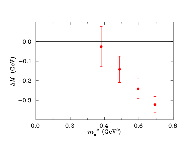
Figure 1: Mass difference between the lowest-lying negative parity excited nucleon bound state, the $I(J^{P})={1\over 2}({1\over 2}^{-})\ N^{*}(1535)$, and the S-wave $N+\pi$ two-particle scattering state.

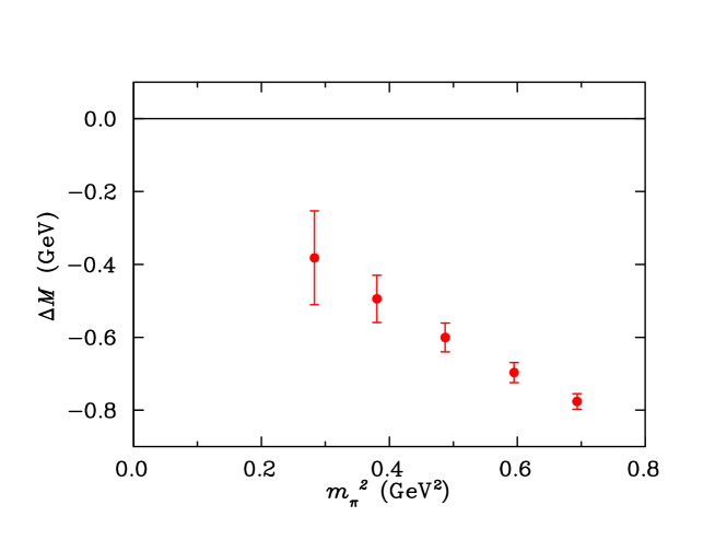
Figure 2: Mass difference between the $I(J^{P})={3\over 2}({3\over 2}^{+})\ \Delta(1232)$ and the $P$-wave $N+\pi$ two-particle scattering state.

As an example, consider the $J^{P}={1\over 2}^{-}$ parity partner of the nucleon, namely the $N^{*}(1535)$ baryon, in lattice QCD. In the continuum, the $N^{*}(1535)$ is a resonance which decays to a nucleon and a pion. On the lattice, however, the $N^{*}({1\over 2}^{-})$ is stable at the (unphysically) large quark masses where its mass is smaller than the sum of the nucleon and pion masses Melnitchouk et al. (2003). To illustrate this we show in Fig. 1 the mass splitting between the $N^{*}({1\over 2}^{-})$ and the non-interacting S-wave $N+\pi$ two-particle state, calculated on the same lattice. For all values of $m_{\pi}$ illustrated the mass of the $N^{*}({1\over 2}^{-})$ is below that of the $N+\pi$, and the mass difference clearly increases in magnitude with increasing $m_{\pi}$. In other words, the binding becomes stronger at larger quark masses.

A similar behaviour is also observed in the case of the $\Delta(1232)$ isobar. The mass difference between the $J^{P}={3\over 2}^{+}$ resonance and the lowest available P-wave $N+\pi$ two-particle energy, shown in Fig. 2, is negative, and, as in Fig. 1, increases with $m_{\pi}^{2}$. In fact, this pattern is repeated in every other baryon channel probed in lattice QCD, such as the $J^{P}={1\over 2}^{+}$ and ${3\over 2}^{-}$ channels, for example Leinweber et al. (2004a); Melnitchouk et al. (2003); Zanotti et al. (2003). Thus the standard lattice resonance signature for the $\Theta^{+}$ resonance is the existence of a state with a mass which becomes smaller than that of the $N+K$ two-particle state as the quark mass increases, with the mass difference increasing at larger quark masses.

IV.2 Negative parity isoscalar states

We begin our discussion of the results with the isospin-0, negative parity states. The lowest energy of a system with a nucleon and a kaon would have the $N$ and $K$ in a relative S-wave, in which case the overall parity is negative. Isoscalar states can be constructed with the $NK$-type interpolating fields, $\chi_{NK}$ and $\chi_{\widetilde{NK}}$, as well as with the $PS$-type field $\chi_{PS}$.

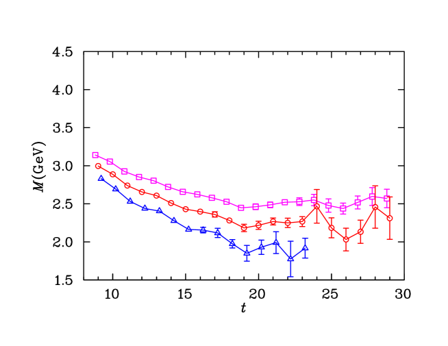
Figure 3: Effective mass of the $I(J^{P})=0(\frac{1}{2}^{-})$ colour singlet $NK$-type pentaquark interpolator, $\chi_{NK}$. The data correspond to $\kappa=1.2780$ (squares), 1.2885 (circles), and 1.2990 (triangles).

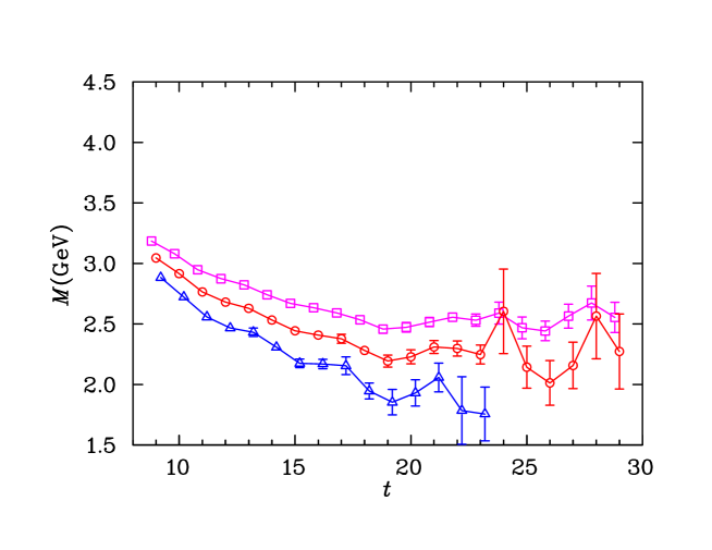
Figure 4: As in Fig. 3, but for the $I(J^{P})=0(\frac{1}{2}^{-})$ colour fused $NK$-type pentaquark interpolator, $\chi_{\widetilde{NK}}$.

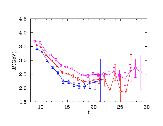
Figure 5: As in Fig. 3, but for the $I(J^{P})=0(\frac{1}{2}^{-})$ $PS$-type pentaquark interpolator, $\chi_{PS}$.

The effective mass for the colour singlet $\chi_{NK}$ field is shown in Fig. 3 for several representative $\kappa$ values. The results for the colour fused operator $\chi_{\widetilde{NK}}$ of Fig. 4 are very similar to those for $\chi_{NK}$. (Note that to avoid clutter in the figures we do not show the points at the larger $t$ values which have larger error bars, and have little influence on the fits.) To determine whether these operators have significant overlap with more than one state, a correlation matrix analysis is performed. However, we find that it is not possible to improve the ground state mass as described in Sec. III.2. Consequently the results using the standard (i.e., non-correlation matrix) analysis techniques are reported in this channel. For comparison, in Fig. 5 we also show the effective mass of the negative parity $\chi_{PS}$ diquark-type field. As expected, because of the presence of two smaller components of Dirac spinors in $\chi_{PS}$ compared with $\chi_{NK}$ and $\chi_{\widetilde{NK}}$ , the signal here is much noisier than for either of the $NK$-type fields. This is despite the fact that almost twice as many configurations are used for the $\chi_{PS}$ than for the $NK$-type fields.

The pentaquark masses are extracted by fitting the effective masses in Figs. 3–5 over appropriate $t$ intervals, chosen according to the criterion that the $\chi^{2}$ per degree of freedom is less than 1.5, and preferably close to 1.0. For the $\chi_{NK}$ and $\chi_{\widetilde{NK}}$ fields, fitting the effective mass in the window $t=19-23$ is found to optimise the $\chi^{2}$/dof. For the $\chi_{PS}$ field, the signal is lost at slightly earlier times, and consequently we fit in the time interval $t=18-20$. The results for the masses corresponding to the $\chi_{NK}$, $\chi_{\widetilde{NK}}$ and $\chi_{PS}$ fields are tabulated in Table 1.

Table 1: The pion mass and the masses of the $I(J^{P})=0(\frac{1}{2}^{-})$ states extracted with the colour singlet $NK$, colour fused $\widetilde{NK}$ and $PS$-type pentaquark interpolating fields for various values of $\kappa$.

$\kappa$	$aM_{\pi}$	$aM_{NK}$	$aM_{\widetilde{NK}}$	$aM_{PS}$
1.2780	0.540(2)	1.612(17)	1.625(16)	1.601(21)
1.2830	0.500(2)	1.539(17)	1.553(16)	1.532(23)
1.2885	0.453(2)	1.449(20)	1.461(20)	1.458(27)
1.2940	0.400(3)	1.349(28)	1.361(29)	1.396(37)
1.2990	0.345(3)	1.236(50)	1.245(48)	1.372(72)
1.3025	0.300(3)	1.145(67)	1.138(80)	1.442(171)

Table 2: Masses of the S-wave $N+K$, $N+K^{*}$, $\Delta+K^{*}$ and $N^{\prime}+K$ two-particle states.

$\kappa$	$aM^{\rm S-wave}_{N+K}$	$aM^{\rm S-wave}_{N+K^{*}}$	$aM^{\rm S-wave}_{\Delta+K^{*}}$	$aM^{\rm S-wave}_{N^{\prime}+K}$
1.2780	1.553(10)	1.762(14)	1.893(13)	2.180(27)
1.2830	1.485(11)	1.704(16)	1.848(14)	2.136(32)
1.2885	1.404(13)	1.635(19)	1.799(16)	2.092(39)
1.2940	1.314(18)	1.561(26)	1.751(19)	2.061(54)
1.2990	1.216(32)	1.485(41)	1.709(24)	2.056(87)
1.3025	1.130(52)	1.421(68)	1.682(29)	2.093(144)

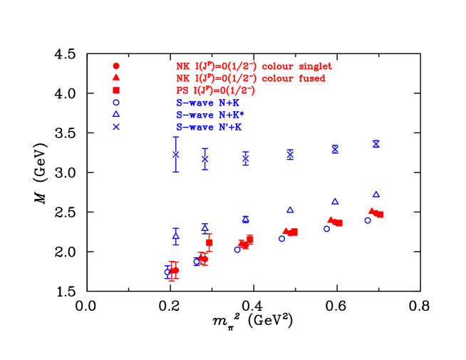
Figure 6: Masses of the $I(J^{P})=0(\frac{1}{2}^{-})$ states extracted with the colour singlet $NK$, colour fused $\widetilde{NK}$ and $PS$-type pentaquark interpolating fields as a function of $m_{\pi}^{2}$. For comparison, the masses of the S-wave $N+K$, $N+K^{*}$ and $N^{\prime}+K$ two-particle states are also shown. Some of the points have been offset for clarity.

The pentaquark masses are compared with masses of several two-particle states, which are reported in Table 2. The lowest-energy two-particle states in the $I(J^{P})=0(\frac{1}{2}^{-})$ channel are the S-wave $N+K$, the S-wave $N+K^{*}$, the P-wave $N^{*}+K$, where $N^{*}$ is the lowest negative parity excitation of the nucleon, and the S-wave $N^{\prime}+K$, where $N^{\prime}$ is the first positive-parity excited state of the nucleon. The contributions to the correlation function from the P-wave states are likely to be suppressed, however, because there is a contribution to the P-wave signal from two small components of the spinors. We therefore focus on the S-wave states in Table 2.

The positive parity $N^{\prime}$ state, which is calculated from the interpolating field $\epsilon^{abc}(u^{aT}Cd^{b})\gamma_{5}u^{c}$, is known to have poor overlap with the nucleon ground state, as well as with the low-lying ${1\over 2}^{+}$ excitations, such as the Roper $N^{*}(1440)$. In fact, it gives a mass greater than $\sim 2$ GeV, significantly above the low-lying ${1\over 2}^{+}$ excitations Melnitchouk et al. (2003). We expect, therefore, that our pentaquark fields will not have strong overlap with the $N^{\prime}+K$ state either.

The results for the extracted masses from Table 1 are displayed in Fig. 6 as a function of $m_{\pi}^{2}$. The masses of the pentaquark states extracted from the $\chi_{NK}$, $\chi_{\widetilde{NK}}$ and $\chi_{PS}$ fields agree within the errors (the $\chi_{NK}$ and $\chi_{\widetilde{NK}}$ masses in particular are very close), although the errors on the $\chi_{PS}$ become large at the smaller quark masses. The pentaquark masses are either consistent with or lie above the mass of the lowest two-particle state, namely the S-wave $N+K$.

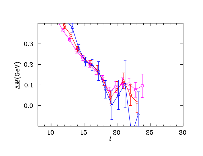
Figure 7: Effective mass difference between the $I(J^{P})=0(\frac{1}{2}^{-})$ state extracted with the colour singlet $NK$-type pentaquark interpolator, $\chi_{NK}$, and the S-wave $N+K$ two-particle state. The data correspond to $\kappa=1.2780$ (squares), 1.2885 (circles), and 1.2990 (triangles).

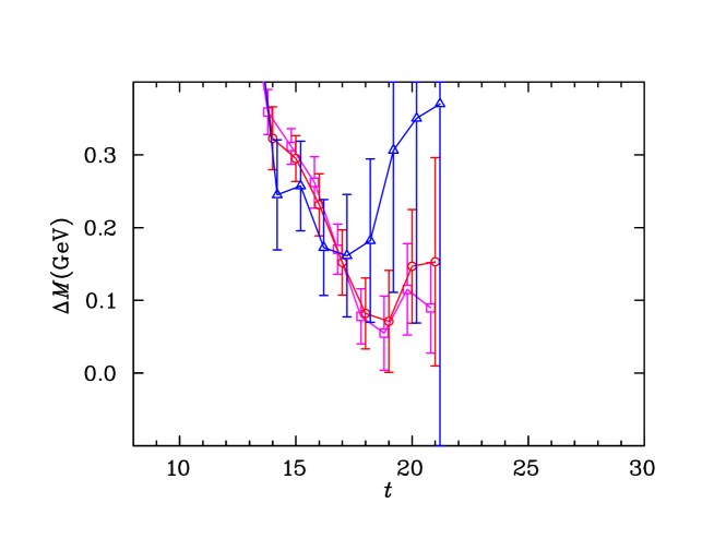
Figure 8: As in Fig. 7, but for the $I(J^{P})=0(\frac{1}{2}^{-})$ $PS$-type interpolating field, $\chi_{PS}$.

Table 3: Mass differences between the $I(J^{P})=0(\frac{1}{2}^{-})$ states extracted with the $NK$ and $PS$-type pentaquark interpolating fields and the S-wave $N+K$ two-particle state.

$\kappa$	$aM_{NK}-aM_{N+K}^{\rm S-wave}$	$aM_{PS}-aM_{N+K}^{\rm S-wave}$
1.2780	0.056(9)	0.051(19)
1.2830	0.052(11)	0.052(21)
1.2885	0.048(13)	0.060(25)
1.2940	0.043(17)	0.086(37)
1.2990	0.025(30)	0.148(75)
1.3025	-0.011(67)	0.286(177)

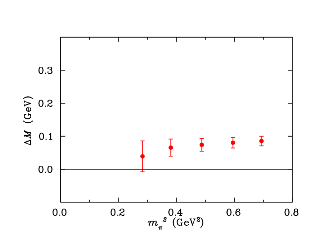
Figure 9: Mass difference between the $I(J^{P})=0(\frac{1}{2}^{-})$ state extracted with the $NK$-type pentaquark interpolating field and the S-wave $N+K$ two-particle state.

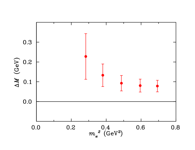
Figure 10: Mass difference between the $I(J^{P})=0(\frac{1}{2}^{-})$ state extracted with the $PS$-type pentaquark interpolating field and the S-wave $N+K$ two-particle state.

The mass differences $\Delta M$ between the low-lying pentaquark states and the two-particle scattering states can be better resolved by fitting the effective mass for the mass difference directly. This allows for cancellation of systematic errors since the pentaquark and two-particle states are generated from the same gauge field configurations, and hence their systematic errors are strongly correlated. Figures 7 and 8 illustrate the effective mass plots for the mass differences. Note that the scale of these figures is enlarged by a factor of six compared with Figs. 3–5. The mass difference between the state extracted from the colour singlet $NK$ interpolator and the S-wave $N+K$ two-particle state is fitted at time slices $t=19-21$, while that between the $PS$ extracted state and the $N+K$ state is fitted at $t=18-20$.

The results of the mass difference analysis are presented in Table 3, and in Figs. 9 and 10 for the $\chi_{NK}$ and $\chi_{PS}$ fields, respectively. We see clearly that the masses derived from the $NK$ pentaquark operator are consistently higher than the lowest-mass two-particle state. The mass difference $\Delta M$ is $\sim 100$ MeV at the larger quark masses, and weakly dependent on $m_{\pi}^{2}$, with a possible trend towards a larger $\Delta M$ with increasing $m_{\pi}^{2}$. Note the size of the error bars for the mass difference is reduced compared with the error bars on the masses in Fig. 6.

Since the difference between the reported experimental $\Theta^{+}$ mass and the physical S-wave $N+K$ continuum is $\sim 100$ MeV, naively one may be tempted to interpret the results in Figs. 9 and 8 as a signature of the $\Theta^{+}$ on the lattice. However, the behaviour of the pentaquark–$(N+K)$ mass difference is in marked contrast to that of all other excited $N^{*}$ states studied on the lattice Melnitchouk et al. (2003); Zanotti et al. (2003); Leinweber et al. (2004a), as discussed in Sec. IV.1 above, for which $\Delta M$ is negative. The lack of any binding leads us to conclude that the observed signal is unlikely to be a resonance, and may instead correspond to an $N+K$ two-particle state. The volume dependent analysis in Ref. Mathur et al. (2004) indeed concluded that their signal, which is consistent with our results, corresponds to an $NK$ scattering state.

IV.3 Negative parity isovector states

For the isospin-1, negative parity sector, we consider three operators which can create $I(J^{P})=1({1\over 2}^{-})$ states: the isovector combinations of the colour singlet $\chi_{NK}$ and colour fused $\chi_{\widetilde{NK}}$, and the $SS$-type operator, $\chi_{SS}$. As for the isoscalar case, we perform a $2\times 2$ correlation matrix analysis for the $NK$-type fields, and here we do find improved access to the lowest lying state.

Using the paradigm for optimising the results described in Sec. III.2, we perform the correlation matrix analysis for the largest 4 quark masses starting at $t=20$ with $\Delta t=3$. Here the ground state mass is found to be lower with the correlation matrix than with the standard analysis, indicating that the contamination of the ground state from excited states is reduced. For the second lightest quark mass we fit at $t=18$, and for the lightest quark mass at $t=17$, with $\Delta t=3$ in both cases. For these two lightest quark masses, the ground state mass is not lowered, so here the standard analysis techniques are used. For the excited state, the masses from the correlation matrix are all higher than with the naive analysis for all quark masses, thus improving the analysis.

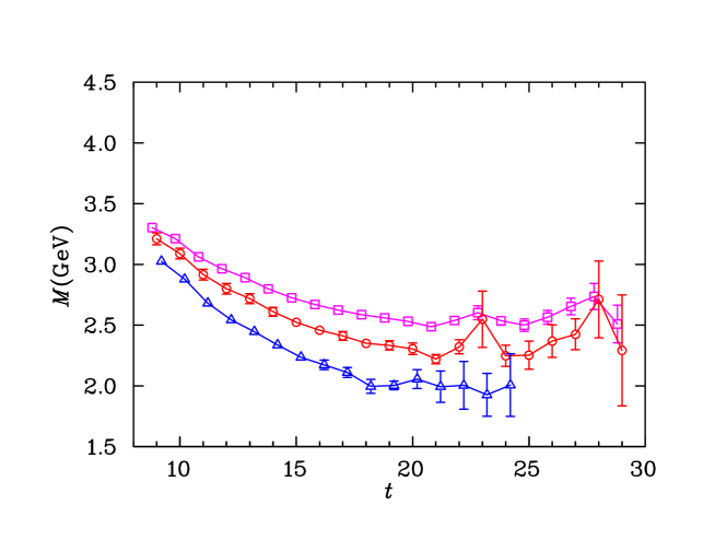
Figure 11: Effective mass of the $I(J^{P})=1(\frac{1}{2}^{-})$ state corresponding to the $NK$-type pentaquark “state 1” for several values of $\kappa$, $\kappa=1.2780$ (squares), 1.2885 (circles), and 1.2990 (triangles).

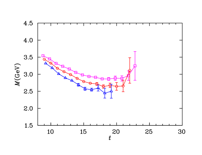
Figure 12: As in Fig. 11, but for the $I(J^{P})=1(\frac{1}{2}^{-})$ $NK$-type pentaquark “state 2”.

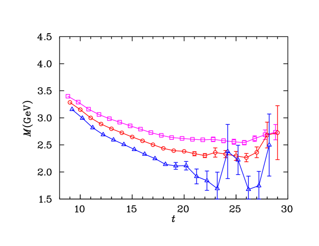
Figure 13: As in Fig. 11, but for the $I(J^{P})=1(\frac{1}{2}^{-})$ $SS$-type interpolator, $\chi_{SS}$.

The effective masses for the two projected $NK$-type correlation matrix states, which we refer to as “state 1” (for the ground state) and “state 2” (for the excited state), are shown in Figs. 11 and 12, respectively. For comparison, we also show the effective mass plot for the $SS$-type field $\chi_{SS}$ in Fig. 13. The ground state mass extracted with the $NK$-type interpolator is fitted at time slices $t=22-26$, while the mass extracted with the $SS$-type interpolator is fitted at time slices $t=19-28$.

Table 4: Masses of the $I(J^{P})=1(\frac{1}{2}^{-})$ states extracted with the $NK$ and $SS$-type pentaquark interpolating fields for various values of $\kappa$.

$\kappa$	$aM_{NK(1)}$	$aM_{NK(2)}$	$aM_{SS}$
1.2780	1.649(15)	1.859(22)	1.692(8)
1.2830	1.578(18)	1.797(25)	1.619(9)
1.2885	1.497(27)	1.720(31)	1.530(11)
1.2940	1.408(48)	1.629(47)	1.434(16)
1.2990	1.313(66)	1.577(77)	1.334(26)
1.3025	1.251(144)	1.554(175)	1.245(51)

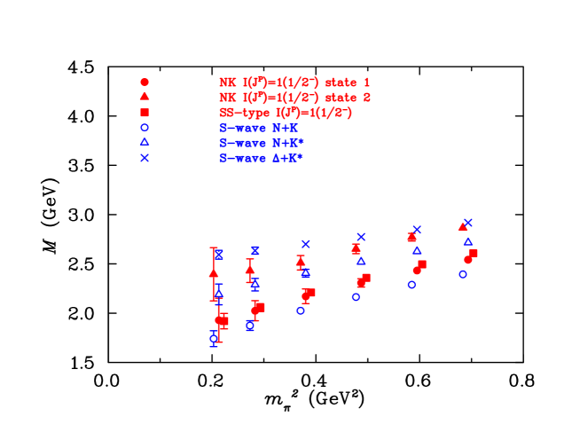
Figure 14: Masses of the $I(J^{P})=1(\frac{1}{2}^{-})$ states extracted with the $NK$ and $SS$-type pentaquark interpolating fields as a function of $m_{\pi}^{2}$, compared with the masses of the S-wave $N+K$, $N+K^{*}$ and $\Delta+K^{*}$ two-particle states. Some of the points have been offset for clarity.

The resulting extracted masses are tabulated in Table 4 and shown in Fig. 14. A clear mass splitting of $\sim 400$ MeV is seen between the ground state and the excited state for the $NK$-type operators. The ground state mass is consistent with that obtained from the $\chi_{SS}$ operator for the four smallest quark masses, but is slightly smaller for the two largest quark masses. As for the isoscalar channel, the ground state masses are either consistent with or slightly above the masses of the lowest two-particle state, the S-wave $N+K$. The excited state lies slightly above the S-wave two-particle $N+K^{*}$ threshold, which suggests that it may be an admixture of $N+K^{*}$ and $\Delta+K^{*}$ scattering states.

Table 5: Mass differences between the $I(J^{P})=1(\frac{1}{2}^{-})$ states extracted with the $NK$ and $SS$-type pentaquark interpolating fields and the S-wave $N+K$, $N+K^{*}$ and $N+K$ two-particle states, respectively.

$\kappa$	$aM_{NK(1)}-aM_{N+K}^{\rm S-wave}$	$aM_{NK(2)}-aM_{N+K^{*}}^{\rm S-wave}$	$aM_{SS}-aM_{N+K}^{\rm S-wave}$
1.2780	0.067(9)	0.109(16)	0.100(11)
1.2830	0.063(13)	0.106(18)	0.090(15)
1.2885	0.059(21)	0.099(24)	0.071(20)
1.2940	0.056(35)	0.082(39)	0.048(26)
1.2990	-0.006(53)	0.102(76)	-0.030(78)
1.3025	-0.161(223)	0.146(176)	-0.021(75)

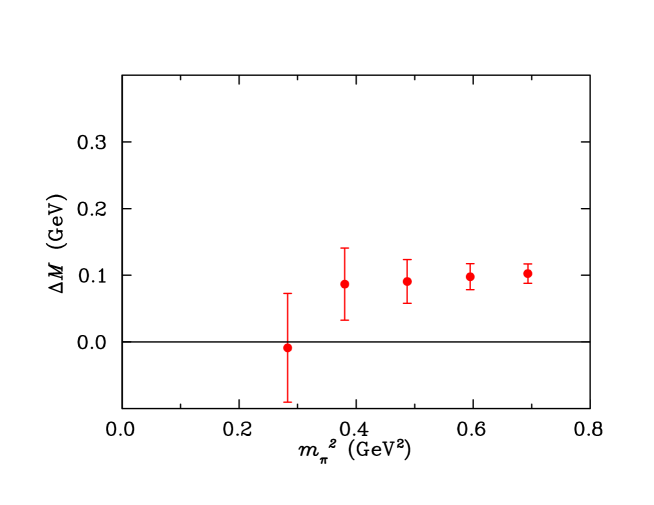
Figure 15: Mass difference between the $I(J^{P})=1(\frac{1}{2}^{-})$ state corresponding to the $NK$-type pentaquark “state 1” and the S-wave $N+K$ two-particle state.

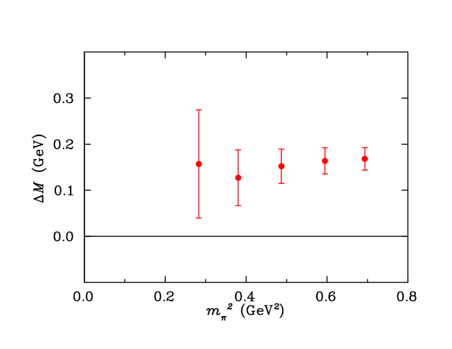
Figure 16: Mass difference between the $I(J^{P})=1(\frac{1}{2}^{-})$ state corresponding to the $NK$-type pentaquark “state 2” and the S-wave $N+K^{*}$ two-particle state.

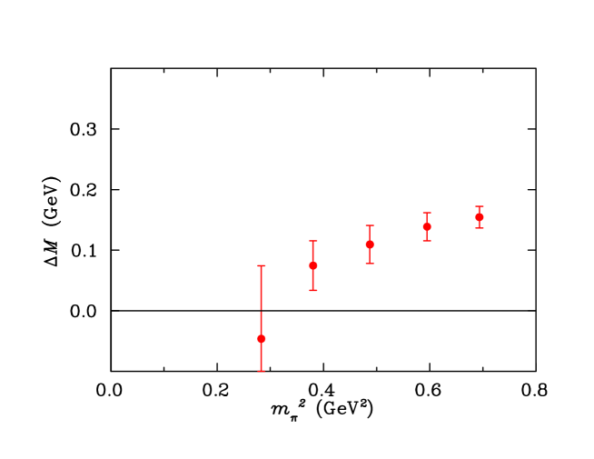
Figure 17: Mass difference between the $I(J^{P})=1(\frac{1}{2}^{-})$ state extracted with the $SS$-type pentaquark interpolating field and the S-wave $N+K$ two-particle state.

The fitted mass differences between the pentaquark and two-particle state effective masses are summarised in Table 5, where we quote the differences between the $NK$-type “state 1” and the S-wave $N+K$, between the $NK$-type “state 2” and the S-wave $N+K^{*}$, and between the $SS$-type and the S-wave $N+K$. These mass differences are illustrated in Figs. 15, 16 and 17, for the three cases, respectively. As for the isoscalar channel, the mass differences for the ground state are clearly positive, and weakly dependent on $m_{\pi}^{2}$. For both the $NK$-type and $SS$-type ground states, the pentaquark masses are $\sim 100$ MeV larger than the S-wave $N+K$ two-particle state. Similarly, the difference between the excited $NK$-type pentaquark and the S-wave $N+K^{*}$ is $\sim 150$ MeV and approximately constant with $m_{\pi}^{2}$. In fact, Figs. 15 and 17 suggest that the $\sim 100$ MeV mass splitting obtained at the largest quark mass considered is approached from below. There is no evidence of binding and no indication of a resonance in the $I(J^{P})=1({1\over 2}^{-})$ channel which could be interpreted as the $\Theta^{+}$.

IV.4 Positive parity isoscalar states

While each of the pentaquark operators considered above transforms negatively under parity, they nevertheless couple to both negative and positive parity states, as discussed in Sec. III.1. Here we consider whether any of the operators $\chi_{NK}$, $\chi_{\widetilde{NK}}$ or $\chi_{PS}$ couple to a bound state in the isospin-0, positive parity channel. We compare the pentaquark states with the masses of the lowest energy two-particle states, which correspond to the P-wave $N+K$ and $N+K^{*}$, and the S-wave $N^{*}+K$ states.

A two-particle state in a relative P-wave can be constructed on the lattice by adding one unit of lattice momentum ($p=2\pi/L$) to the effective mass, $E_{\rm eff}=\sqrt{M_{\rm eff}^{2}+p^{2}}$, of each particle. This effectively raises the mass of the two-particle state relative to the positive parity pentaquark. If a pentaquark state exists, it should therefore clearly lie below the lowest P-wave scattering state.

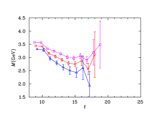
Figure 18: Effective mass of the $I(J^{P})=0(\frac{1}{2}^{+})$ colour singlet $NK$-type pentaquark interpolator, $\chi_{NK}$, for $\kappa=1.2780$ (squares), 1.2885 (circles) and 1.2990 (triangles).

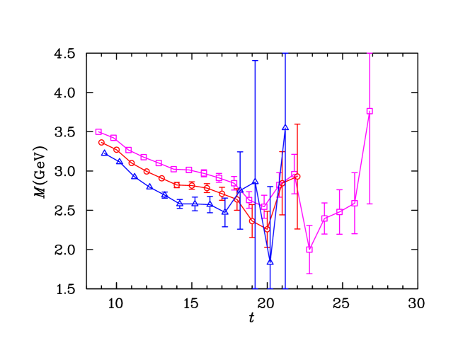
Figure 19: As in Fig. 18, but for the $I(J^{P})=0(\frac{1}{2}^{+})$ $PS$-type pentaquark interpolator, $\chi_{PS}$.

As in the negative parity channel, we perform a correlation matrix analysis using the two $NK$-type fields in order to isolate possible excited states. While the analysis suggests the presence of an excited state, the signal in the positive parity channel is considerably more noisy than for negative parity. Consequently, in practice for this channel we revert to the standard analysis method and extract only the ground state. Since the colour singlet and colour fused operators return the same ground state mass, we present the results for the colour singlet operator since the signal here is less noisy.

Table 6: Masses of the $I(J^{P})=0(\frac{1}{2}^{+})$ states extracted with the colour singlet $NK$, and $PS$-type pentaquark interpolating fields for various values of $\kappa$.

$\kappa$	$aM_{NK}$	$aM_{PS}$
1.2780	1.935(40)	1.721(57)
1.2830	1.867(50)	1.642(76)
1.2885	1.782(66)	1.547(119)
1.2940	1.681(90)	1.458(207)
1.2990	1.561(126)
1.3025	1.421(170)

Table 7: The masses of the P-wave $N+K$, $N+K^{*}$ and the S-wave $N^{*}+K$ two-particle states.

$\kappa$	$aM^{\rm P-wave}_{N+K}$	$aM^{\rm S-wave}_{N+K^{*}}$	$aM^{\rm S-wave}_{N^{*}+K}$
1.2780	1.692(7)	1.891(27)	1.873(9)
1.2830	1.629(8)	1.830(32)	1.818(9)
1.2885	1.558(8)	1.760(39)	1.755(10)
1.2940	1.483(10)	1.684(53)	1.690(11)
1.2990	1.414(13)	1.594(85)	1.631(14)
1.3025	1.363(17)	1.433(134)	1.588(17)

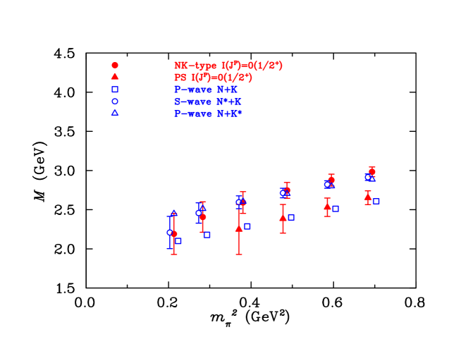
Figure 20: Masses of the $I(J^{P})=0(\frac{1}{2}^{+})$ states extracted with the colour singlet $NK$ and $PS$-type pentaquark interpolating fields as a function of $m_{\pi}^{2}$. For comparison, the masses of the P-wave $N+K$ and $N+K^{*}$ and S-wave $N^{*}+K$ two-particle states are also shown. Some of the points have been offset for clarity.

The effective masses for the $NK$ and $PS$-type interpolators are shown in Figs. 18 and 19, respectively. The signal clearly becomes noisier at earlier times, and we fit the effective masses for the $NK$-type field at $t=15-17$, while those for the $PS$-type interpolator are fit at $t=19-21$.

Table 8: Mass differences between the $I(J^{P})=0(\frac{1}{2}^{+})$ states extracted with the colour singlet $NK$ and $PS$-type pentaquark interpolating fields and the P-wave $N+K$ two-particle state.

$\kappa$	$aM_{NK}-aM^{\rm P-wave}_{N+K}$	$aM_{PS}-aM^{\rm P-wave}_{N+K}$
1.2780	0.228(38)	0.035(57)
1.2830	0.223(48)	0.021(78)
1.2885	0.209(65)	0.003(122)
1.2940	0.183(90)	-0.003(210)
1.2990	0.132(128)
1.3025	0.040(174)

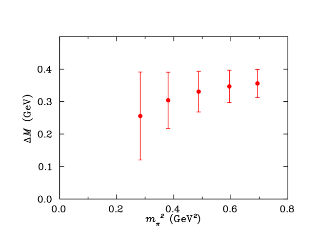
Figure 21: Mass difference between the $I(J^{P})=0(\frac{1}{2}^{+})$ state extracted with the $NK$-type pentaquark interpolating field and the P-wave $N+K$ two-particle state.

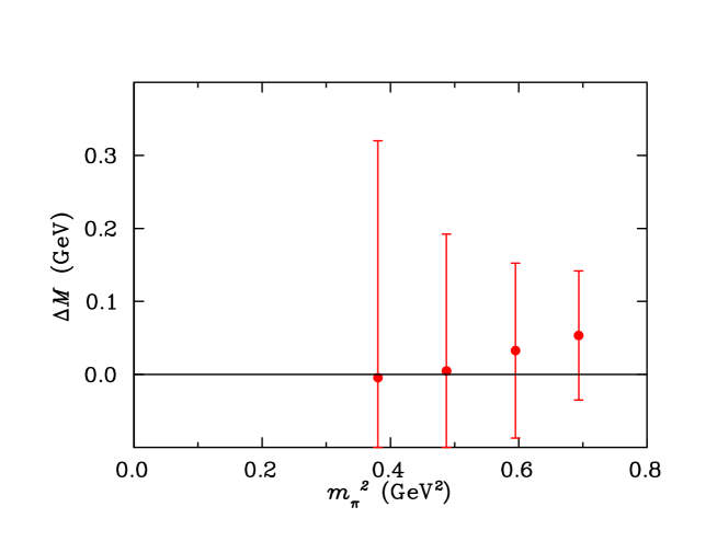
Figure 22: Mass difference between the $I(J^{P})=0(\frac{1}{2}^{+})$ state extracted with the $PS$-type pentaquark interpolating field and the P-wave $N+K$ two-particle state.

The results are tabulated in Table 6 and shown in Fig. 20. The masses of the positive parity states extracted with the $NK$ and $PS$-type interpolating fields are very different. The mass extracted with the $NK$-type interpolator is similar to both the S-wave $N^{*}+K$ mass and P-wave $N+K^{*}$ energy, whereas the mass extracted with the $PS$-type interpolator is consistent with the P-wave $N+K$ energy, which are given in Table 8. The signal obtained with the $PS$-type interpolator is rather noisy where we fit the effective masses, and we therefore only present results for the four largest quark masses for this operator. As mentioned in Sec. IV.2, the reason the signal is so poor is that our operators do not couple strongly to the P-wave states due to the additional small component of the interpolating field spinors contributing to this state.

For the differences between the pentaquark and two-particle state masses, we also fit the effective masses at $t=15-17$ for the $NK$-type field, and $t=19-21$ for the $PS$-type field. The results are shown in Table 8, and in Figs. 21 and 22 for the differences between the masses extracted with the ($NK$ and $PS$-type) pentaquark interpolating fields and the P-wave $N+K$ two-particle state. The mass obtained with the $NK$-type field is $\sim 300$ MeV heavier than the lowest energy two-particle state (P-wave $N+K$) for all quark masses considered. The mass obtained with the $PS$-type field is consistent with the the lowest energy two-particle state (P-wave $N+K$) for all quark masses considered. Once again this suggests that there is no binding in the $I(J^{P})=0(\frac{1}{2}^{+})$ channel, and hence no indication of a $\Theta^{+}$ resonance.

IV.5 Positive parity isovector states

For the isospin-1, positive parity channel analysis, we find that the correlation matrix does not produce improved results for the ground state masses compared with the standard analysis. In the case of the largest three $\kappa$ values the algorithm requires that we step back three or more time slices before the correlation matrix analysis works. The use of a correlation matrix analysis on these data is inappropriate due to large errors in the data.

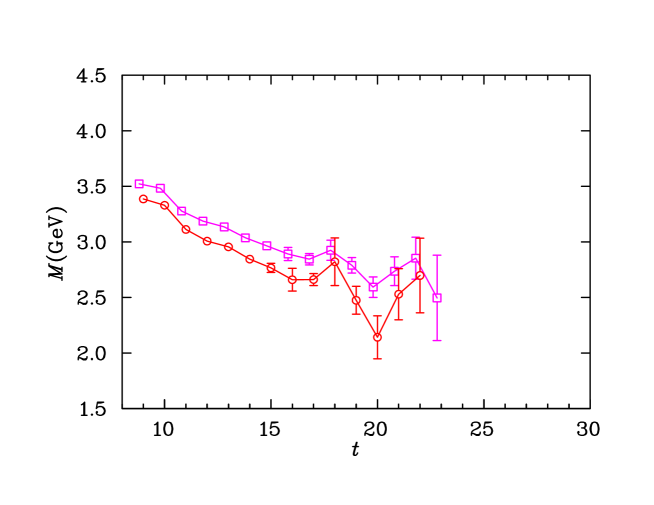
Figure 23: Effective mass of the $I(J^{P})=1(\frac{1}{2}^{+})$ colour singlet $NK$-type pentaquark interpolator, $\chi_{NK}$. The data correspond to $\kappa=1.2780$ (squares) and 1.2885 (circles).

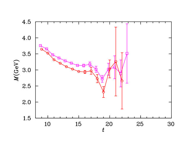
Figure 24: As in Fig. 23, but for the $I(J^{P})=1(\frac{1}{2}^{+})$ $SS$-type pentaquark interpolator, $\chi_{SS}$.

The effective masses for the $NK$-type and $SS$-type interpolating fields are illustrated in Figs. 23 and 24, respectively. Because the signal for the positive parity is rather more noisy than in the corresponding negative parity channel, we only show the effective mass for the smallest and third-smallest values of $\kappa$. For the $NK$-type pentaquarks, the colour-singlet $\chi_{NK}$ and colour-fused $\chi_{\widetilde{NK}}$ fields are found to access the same ground state, and in Fig. 23 we only show the results of the former.

Table 9: Masses of the $I(J^{P})=1(\frac{1}{2}^{+})$ states extracted with the colour singlet $NK$ and $SS$-type pentaquark interpolating fields for various values of $\kappa$.

$\kappa$	$aM_{NK}$	$aM_{SS}$
1.2780	1.732(48)	1.956(133)
1.2830	1.651(57)	1.939(158)
1.2885	1.536(71)	1.954(214)

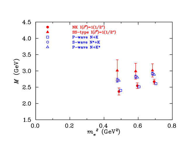
Figure 25: Masses of the $I(J^{P})=1(\frac{1}{2}^{+})$ states extracted with the colour singlet $NK$ and $SS$-type pentaquark interpolating fields as a function of $m_{\pi}^{2}$. For comparison, the masses of the P-wave $N+K$, S-wave $N^{*}+K$ and P-wave $N+K^{*}$ two-particle states are also shown. Some of the points have been offset for clarity.

The effective masses for the $NK$ and $SS$-type interpolators are fitted at time slices $t=20-22$ for the three largest quark masses. The results for the extracted masses and the corresponding two-particle states are shown in Table 9 and in Fig. 25. The ground state masses for the $NK$ and $SS$-type fields are again very different. The mass extracted with the $NK$-type interpolator is consistent with the P-wave $N+K$ energy, whereas the mass extracted with the $SS$-type interpolator is consistent with both the S-wave $N^{*}+K$ mass and P-wave $N+K^{*}$ energy.

Table 10: Mass differences between the $I(J^{P})=1(\frac{1}{2}^{+})$ states extracted with the colour singlet $NK$ and $SS$-type pentaquark interpolating fields and P-wave $N+K$ two-particle state.

$\kappa$	$aM_{NK}-aM^{\rm P-wave}_{N+K}$	$aM_{SS}-aM^{\rm P-wave}_{N+K}$
1.2780	0.093(43)	0.135(58)
1.2830	0.079(53)	0.117(61)
1.2885	0.034(70)	0.084(69)

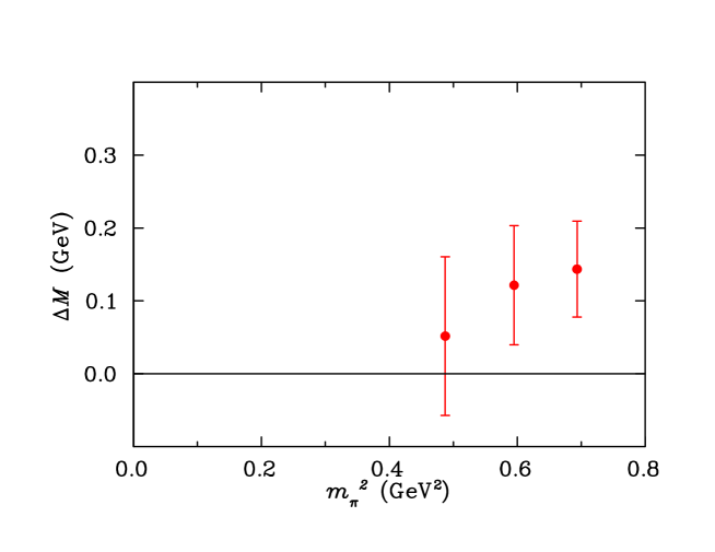
Figure 26: Mass difference between the $I(J^{P})=1(\frac{1}{2}^{+})$ state extracted with the $NK$-type pentaquark interpolating field and the P-wave $N+K$ two-particle state.

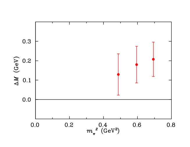
Figure 27: Mass difference between the $I(J^{P})=1(\frac{1}{2}^{+})$ state extracted with the $SS$-type pentaquark interpolating field and the P-wave $N+K$ two-particle state.

The results of the mass splitting analysis are shown in Table 10, and illustrated in Figs. 26 and 27. The mass difference between the $NK$ and $SS$-type pentaquarks and the P-wave $N+K$ two-particle state is positive for the largest quark masses. The splitting increases with $m_{\pi}^{2}$, giving an indication of repulsion, rather than attraction. In all cases, the masses exhibit the opposite behaviour to that which would be expected in the presence of binding. We therefore do not see any indication of a resonance that could be interpreted as the $\Theta^{+}$ in this channel.

IV.6 Comparison with previous results

To place our results in context, we summarise here the results of earlier lattice calculations of pentaquark masses, and compare those with the findings of this analysis. Table 11 presents a concise summary of published lattice simulations, together with the results of this analysis, including the actions and interpolating fields used, analysis methods employed, and some remarks on the results. In every case, the general features of the simulation results are consistent with our findings.

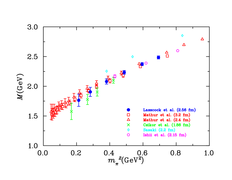
Figure 28: Compilation of results for the lowest-lying $I(J^{P})=0(\frac{1}{2}^{-})$ state from lattice QCD pentaquark studies.

The isoscalar negative parity channel was originally presented by Csikor et al. Csikor et al. (2003) and Sasaki Sasaki (2004a) as a candidate for the $\Theta^{+}$. We therefore summarise in Fig. 28 the results in this channel from the previous lattice simulations. At the larger quark masses the results of our analysis are in excellent agreement with those of Mathur et al. Mathur et al. (2004), Csikor et al. Csikor et al. (2003) and Ishii et al. Ishii et al. (2005, 2004). In our analysis, and also in that of Mathur et al. Mathur et al. (2004), improved fermion actions were used, and the results are in agreement at the smaller quark masses. The results from Csikor et al. Csikor et al. (2003) lie slightly lower than the others at small quark masses, which may be due to scaling violations of the Wilson fermion action.

The central issue in all of these analyses is the interpretation of the data. The earlier work of Csikor et al. Csikor et al. (2003) and Sasaki Sasaki (2004a) identified the $0({1\over 2}^{-})$ channel as a possible candidate for the $\Theta^{+}$ based on naive linear extrapolations and comparison of quenched QCD with experiment. Later work by Mathur et al. Mathur et al. (2004) analysed the volume dependence of the couplings of the operators to this state and determined that the lowest energy state in this channel was an $N+K$ scattering state. Using hybrid boundary conditions Ishii et al. Ishii et al. (2005, 2004) also found that this was an $N+K$ scattering state. Our work is consistent with the findings of both of these studies.

Table 11: Summary of published lattice QCD pentaquark studies, including the fields used, a brief description of the analysis techniques, and some observations from the work.

Group	Action	Operators	Analysis methods	Observations
Lasscock et al.	FLIC	$\chi_{NK}$, $\chi_{\widetilde{NK}}$,	$2\times 2$ correlation matrix;	$I(J^{P})=1(\frac{1}{2}^{\pm})$ $NK$ scattering states;
		$\chi_{SS}$, $\chi_{PS}$	mass splittings analysis with	$I(J^{P})=0(\frac{1}{2}^{-})$ $NK$ scattering state;
			$NK$, $NK^{*}$	$0(\frac{1}{2}^{+})$ $N^{*}K$ scattering state
Csikor et al. Csikor et al. (2003)	Wilson	$\chi_{NK}$, $\chi_{\widetilde{NK}}$	$2\times 2$ correlation matrix;	$0(\frac{1}{2}^{-})$ $NK$ degenerate state;
			mass ratio with $NK$	$0(\frac{1}{2}^{-})$ excited state, $0(\frac{1}{2}^{+})$ deemed too massive
Sasaki Sasaki (2004a)	Wilson	$\chi_{PS}$	standard analysis	$0(\frac{1}{2}^{-})$ above S-wave $NK$;
				$0(\frac{1}{2}^{+})$ above P-wave $NK$
Mathur et al. Mathur et al. (2004)	overlap	$\chi_{NK}$, $\chi_{\widetilde{NK}}$	volume dependence	$0,1(\frac{1}{2}^{-})$ $NK$ scattering state;
				$0,1(\frac{1}{2}^{+})$ P-wave $NK$ degenerate
Ishii et al. Ishii et al. (2005, 2004)	Wilson	$\chi_{PS}$	hybrid boundary conditions;	$0(\frac{1}{2}^{-})$ $NK$ scattering state;
			Bayesian analysis	$0(\frac{1}{2}^{+})$ deemed too massive
Alexandrou et al. Alexandrou et al. (2004a)	Wilson	$\chi_{PS}$	volume dependence	$0({1\over 2}^{-})$ more consistent with single particle state;
				$NK$ scattering state not seen
Chiu et al. Chiu and Hsieh (2004)	domain wall	$\chi_{NK}$, $\chi_{\widetilde{NK}}$,	$3\times 3$ correlation matrix	$0(\frac{1}{2}^{-})$ $NK$ scattering state;
		$\chi_{PS}$		ground state $0(\frac{1}{2}^{-})$ less massive than $0(\frac{1}{2}^{+})$
Takahashi et al. Takahashi et al. (2004)	Wilson	$\chi_{NK}$, $\chi_{\widetilde{NK}}$	$2\times 2$ correlation matrix;	$\frac{1}{2}^{-}$ $NK$ scattering state;
			volume dependence	$\frac{1}{2}^{-}$ excited state;
				$\frac{1}{2}^{+}$ $N^{*}K$ scattering state

V Conclusion

We have performed a comprehensive analysis of interpolating fields holding the promise to provide good overlap between the the QCD vacuum and low-lying pentaquark states. Central to our analysis is the search for evidence of attraction between the constituents of pentaquark states as the input quark masses increase. Every other baryon resonance ever studied on the lattice becomes stable on the lattice at sufficiently large quark masses. This is the standard resonance signature in lattice QCD. The mass of the resonance becomes less than the sum of the masses of its decay products and is prevented from decaying by energy conservation. Attraction is essential to the formation of a resonance in the light quark mass regime of QCD.

Our results reveal no evidence of attraction that leads to a bound pentaquark state at large quark masses. Rather, evidence of repulsion is evident in the correlation functions giving rise to the lowest-lying pentaquark masses. This is particularly evident in the $I(J^{P})=1(\frac{1}{2}^{-})$ state and in the more accurate results for the $0(\frac{1}{2}^{-})$ state. Similarly, both positive parity states show an increasing mass splitting between pentaquark and two-particle states, again suggesting repulsion as opposed to attraction.

Moreover, in every case where an interpolating field was constructed to favor $J^{P}=\frac{1}{2}^{+}$ states which are more exotic than the colour-singlet paring of a $K$ and $N$, the approach to the lowest-lying state was compromised. In most cases, the same ground state mass was recovered in the correlation function analysis, but with increased error bars. This provides further evidence that the lowest lying state is simply an $NK$ scattering state.

In the case of the $I(J^{P})=1(\frac{1}{2}^{-})$ state, the colour-fused $NK$ interpolator of Eq. (2) had sufficient overlap with an exited state to allow a successful correlation matrix analysis. Again, the exotic colour-fused $NK$ interpolating failed to produce evidence of a bound pentaquark state, the signature of a resonance on the lattice.

Similarly, the scalar diquark-type interpolating field of Eq. (10) produced effective masses that lie higher than those recovered from the colour-singlet $NK$-type interpolating field of Eq. (1). Again, a low-lying pentaquark state was not accessed, indicating the absence of the standard lattice resonance signature. In short, evidence supporting the existence of a spin-${1\over 2}$ pentaquark resonance does not exist in quenched QCD.

This result makes it clear that a similar analysis in full dynamical-fermion QCD is essential to resolving the fate of the putative pentaquark resonance. We have resolved mass splittings of the order of 100 MeV, and one might wonder what effect the dynamics of full QCD could have on this state. As differences in self-energies between full and quenched QCD of order 100 MeV or more have been observed Young et al. (2002), one cannot yet rule out the possible existence of a pentaquark in full QCD.