Effective Actions for the SU(2) Confinement–Deconfinement Phase Transition

Abstract

We compare different Polyakov loop actions yielding effective descriptions of finite–temperature $SU(2)$ Yang–Mills theory on the lattice. The actions are motivated by a simultaneous strong–coupling and character expansion obeying center symmetry and include both Ising and Ginzburg–Landau type models. To keep things simple we limit ourselves to nearest–neighbor interactions. Some truncations involving the most relevant characters are studied within a novel mean–field approximation. Using inverse Monte–Carlo techniques based on exact geometrical Schwinger–Dyson equations we determine the effective couplings of the Polyakov loop actions. Monte–Carlo simulations of these actions reveal that the mean–field analysis is a fairly good guide to the physics involved. Our Polyakov loop actions reproduce standard Yang–Mills observables well up to limitations due to the nearest–neighbor approximation.

I Introduction

The finite–temperature confinement–deconfinement phase transition in $SU(2)$ Yang–Mills theory originally conjectured by Polyakov Polyakov (1978) and Susskind Susskind (1979) is by now fairly well established. The order parameter is the Polyakov loop,

$$L_{\mbox{\scriptsize\boldmath$x$}}\equiv\frac{1}{2}\,\mbox{tr}\,\mathcal{T}\,\exp\Big{(}i\int_{0}^{\beta_{T}}\!\!d\tau\,A^{0}(\mbox{\boldmath$x$},\tau)\Big{)}\;,$$ (1)

a traced Wilson line that winds around the periodic Euclidean time direction parameterized by $\tau$, $0\leq\tau\leq\beta_{T}$ where $\beta_{T}=1/T$ is the inverse temperature. In the confined phase the expectation value $\langle L\rangle$ is zero, while it becomes nonvanishing in the broken, deconfined phase. The Polyakov loop transforms nontrivially under the center symmetry,

$$L_{\mbox{\scriptsize\boldmath$x$}}\to zL_{\mbox{\scriptsize\boldmath$x$}}\;,\quad z=\pm 1\in\mathbb{Z}(2)\;.$$ (2)

Thus, above the critical temperature, $T=T_{c}$, this symmetry becomes spontaneously broken. Lattice calculations have shown beyond any doubt that the phase transition is second order with the critical exponents being those of the 3$d$ Ising model Caselle and Hasenbusch (1996); Gliozzi and Provero (1997); de Forcrand and von Smekal (2003); Pepe and de Forcrand (2002). This is in accordance with the Svetitsky–Yaffe conjecture Svetitsky and Yaffe (1982); Yaffe and Svetitsky (1982) which states in particular that $SU(2)$ Yang–Mills theory (in 4$d$) is in the universality class of a $\mathbb{Z}(2)$ spin model (in $3d$) with short–range interactions. Hence, it should be possible to describe the confinement–deconfinement transition by an effective theory formulated solely in terms of the Polyakov loop $L_{\mbox{\scriptsize\boldmath$x$}}$. The most general ansatz is given by a center–symmetric effective Polyakov loop action (PLA) of the form Svetitsky (1986)

$$S_{\mathrm{PL}}[L] = \sum_{\mbox{\scriptsize\boldmath$x$}}V[L_{\mbox{\scriptsize\boldmath$x$}}^{2}]+\sum_{\mbox{\scriptsize\boldmath$x$}\mbox{\scriptsize\boldmath$y$}}L_{\mbox{\scriptsize\boldmath$x$}}K^{(2)}_{\mbox{\scriptsize\boldmath$x$}\mbox{\scriptsize\boldmath$y$}}L_{\mbox{\scriptsize\boldmath$y$}}$$ (3)

$$+ \sum_{\mbox{\scriptsize\boldmath$x$}\mbox{\scriptsize\boldmath$y$}\mbox{\scriptsize\boldmath$u$}\mbox{\scriptsize\boldmath$v$}}L_{\mbox{\scriptsize\boldmath$x$}}L_{\mbox{\scriptsize\boldmath$y$}}K^{(4)}_{\mbox{\scriptsize\boldmath$x$}\mbox{\scriptsize\boldmath$y$}\mbox{\scriptsize\boldmath$u$}\mbox{\scriptsize\boldmath$v$}}L_{\mbox{\scriptsize\boldmath$u$}}L_{\mbox{\scriptsize\boldmath$v$}}+\ldots$$

There is a potential term $V$, a power series in $L_{\mbox{\scriptsize\boldmath$x$}}^{2}$ living on single lattice sites $x$, plus hopping terms with kernels $K^{(2n)}$ connecting more and more lattice sites $\mbox{\boldmath$x$},\mbox{\boldmath$y$},\ldots$. It is important to note that $L$ is a dimensionless and compact variable, $L_{\mbox{\scriptsize\boldmath$x$}}\in[-1,1]$. Thus, in principle, one is confronted with a proliferation of possible operators that may appear in the PLA (3). One simplification arises due to the Svetitsky–Yaffe conjecture implying that the kernels $K^{(2n)}$ should be short–ranged. Hence, upon expanding like for instance,

$$K^{(2)}_{\mbox{\scriptsize\boldmath$x$}\mbox{\scriptsize\boldmath$y$}}=\sum_{\mbox{\scriptsize\boldmath$r$}}\lambda_{r}\,\delta_{\mbox{\scriptsize\boldmath$y$},\mbox{\scriptsize\boldmath$x$}+\mbox{\scriptsize\boldmath$r$}}\;,$$ (4)

one expects that the first few terms with small $r\equiv|\mbox{\boldmath$x$}-\mbox{\boldmath$y$}|$ will dominate, i.e. will have the largest couplings $\lambda_{r}$. To check this expectation one needs a reliable method to calculate the kernels $K^{(2n)}$ or, equivalently, the coupling parameters inherent in them. A particularly suited approach is introduced in the following section.

II Inverse Monte–Carlo Method

Inverse Monte–Carlo (IMC) is a numerical method to determine effective actions Falcioni et al. (1986); Gonzalez-Arroyo and Okawa (1987). The latter are generically defined via

$$\exp(-S_{\mathrm{eff}}[X])\equiv\int\mathscr{D}U\,\delta(X-X[U])\exp(-S[U])\;,$$ (5)

where the $U$’s represent some ‘microscopic’ degrees of freedom and the $X$’s the effective ‘macroscopic’ ones. In the spirit of Wilson’s renormalization group, these are obtained by integrating out the $U$’s in favor of the $X$’s. It is important to distinguish this ‘Wilsonian’ notion of an effective action from the 1–particle–irreducible (1PI) effective action which will later on be employed as well (cf. the recent remarks in Banks (2004)).

Of course, the problem with (5) is to do the integration nonperturbatively which in general is not possible. In this case, one has to resort to choosing an ansatz like (3) as dictated by symmetry and dimensional counting or to do the integration numerically. The huge number of degrees of freedom involved clearly suggests to use Monte–Carlo (MC) methods. However, this amounts to calculating expectation values rather than integrals like (5). Hence, one needs a recipe to get from expectation values to effective actions. This is exactly what IMC is supposed to do (see Fig. 1).

Figure 1: Illustration of the IMC procedure.

Our particular IMC method is based on the Schwinger–Dyson equations that must hold in the effective theory once a particular ansatz is chosen. In our case, the macroscopic degrees are given by the Polyakov loops $L_{\mbox{\scriptsize\boldmath$x$}}$ distributed according to the PLA $(\ref{in5})$ which we rewrite as

$$S_{\mathrm{PL}}[L]\equiv\sum_{a=1}^{N_{a}}\lambda_{a}S_{a}[L]\;,$$ (6)

with $\mathbb{Z}(2)$ symmetric operators $S_{a}$ and coupling parameters $\lambda_{a}$ to be determined from the Schwinger–Dyson equations. To derive these, we proceed as follows.

On a lattice with spacing $a$ and temporal extent $N_{t}$ (hence temperature $T=1/N_{t}a$) the Polyakov line is given by the product of temporal links,

$$\mathfrak{P}_{\mbox{\footnotesize\boldmath$x$}}\equiv\prod_{t=1}^{N_{t}}U_{\mbox{\scriptsize\boldmath$x$},t;0}\in SU(2)\;.$$ (7)

This $SU(2)$ matrix may be diagonalized whereupon it can be written as

$$\mathfrak{P}_{\mbox{\footnotesize\boldmath$x$}}=\left(\begin{array}[]{cc}\exp(i\theta_{\mbox{\scriptsize\boldmath$x$}})&0\\ 0&\exp(-i\theta_{\mbox{\scriptsize\boldmath$x$}})\end{array}\right)\;,$$

with $-\pi\leq\theta_{\mbox{\scriptsize\boldmath$x$}}\leq\pi$. This representation immediately yields the trace (divided by two),

$$L_{\mbox{\scriptsize\boldmath$x$}}={\textstyle\frac{1}{2}}\mbox{tr}\mathfrak{P}_{\mbox{\footnotesize\boldmath$x$}}=\cos\theta_{\mbox{\scriptsize\boldmath$x$}}\;,$$ (8)

which contains all the gauge invariant information contained in the group variable $\mathfrak{P}_{\mbox{\footnotesize\boldmath$x$}}$. As an aside, we remark that this peculiar feature will no longer be true for higher $SU(N)$ groups Meisinger et al. (2002); Dumitru et al. (2004). In this more general case, traces of $N-1$ different powers of $\mathfrak{P}_{\mbox{\footnotesize\boldmath$$}}$ are required.

With (5) the action (6) leads to the partition function

$$Z=\int\mathscr{D}L\exp(-S_{\mathrm{PL}}[L])\;,$$ (9)

where the integration is performed with the reduced Haar measure $h$ of $SU(2)$,

$$\mathscr{D}L\equiv\prod_{\mbox{\scriptsize\boldmath$x$}}dh\,(L_{\mbox{\scriptsize\boldmath$x$}}),\quad dh(u)=\frac{2}{\pi}\sqrt{1-u^{2}}\,du\;.$$ (10)

Since $S_{\mathrm{PL}}$ depends on the Polyakov loop only via the class function $L_{\mbox{\scriptsize\boldmath$x$}}$ in (8) we may use the left–right invariant Haar measure $\mathscr{D}\mathfrak{P}_{\mbox{\footnotesize\boldmath$$}}$ in (9) instead of the reduced Haar measure. The enhanced symmetry of the measure yields the following geometrical Schwinger-Dyson equations Dittmann et al. (2004),

$$0=\int\mathscr{D}L\,\exp(-S_{\mathrm{PL}})\left[3L_{\mbox{\scriptsize\boldmath$x$}}G-(1-L_{\mbox{\scriptsize\boldmath$x$}}^{2})(G_{\mbox{\scriptsize\boldmath$x$}}^{\prime}-GS_{\mathrm{PL},\mbox{\scriptsize\boldmath$x$}}^{\prime})\right]\;.$$ (11)

Here, $G[L]$ represents some set of functions of the Polyakov loop to be chosen appropriately (see below). In addition, we have defined the derivative $G_{\mbox{\scriptsize\boldmath$x$}}^{\prime}\equiv\partial G/\partial L_{\mbox{\scriptsize\boldmath$x$}}$ and analogously for $S_{\mathrm{PL}}$.

Switching to expectation value notation, (11) can be rewritten as a linear system for the couplings in (6),

$$\sum_{a}\langle(1-L_{\mbox{\scriptsize\boldmath$x$}}^{2})GS^{\prime}_{a,\mbox{\scriptsize\boldmath$x$}}\rangle\lambda_{a}=\langle(1-L_{\mbox{\scriptsize\boldmath$x$}}^{2})G^{\prime}_{\mbox{\scriptsize\boldmath$x$}}\rangle-3\langle L_{\mbox{\scriptsize\boldmath$x$}}G\rangle\;.$$ (12)

The coefficients of this system are expectation values which are calculated in the full Yang–Mills ensemble obtained by MC simulation based on the $SU(2)$ Wilson action. Numerically, it is of advantage to have more equations than unknown couplings $\lambda_{a}$. This is achieved by choosing $G$ out of the following set of local functions,

$$G_{a,\mbox{\scriptsize\boldmath$y$}}\in\{\partial S_{a}/L_{\mbox{\scriptsize\boldmath$y$}}\;,a=1,\ldots,N_{a}\}\;,$$ (13)

which represent the operators present in the equation of motion for $L_{\mbox{\scriptsize\boldmath$y$}}$. For fixed $y$, (12) then yields as many equations as there are couplings, namely $N_{a}$. These equations relate different two–point functions labeled by lattice sites $x$ and $y$ of distance $r$. Additional relations are obtained by letting the distance $r$ run through (half of) the spatial lattice extent, $r=1,\ldots,N_{s}/2$. Altogether, the overdetermined system (12) consists of $N_{a}\times N_{s}/2$ equations which are solved by least–square methods. For more details the reader is referred to Appendix B and Dittmann et al. (2004).

III Character expansion

To find a reasonable choice of operators for the ansatz (6) we use the beautiful analytical results of Billó et al. Billó et al. (1996). These authors have evaluated the integral (5) for the case at hand ($S[U]$ being the Wilson action, $X\equiv L$ the Polyakov loop) by combining the strong–coupling with a character expansion. For the benefit of the reader we briefly recapitulate their approach before we adopt it for our purposes.

Recall that a character is the trace of a group element in an irreducible representation. If $j$ denotes the spin of an $SU(2)$ representation such that $p=2j$ is the length of the corresponding Young tableau, then the associated character is

$$\chi_{p}(U)=\mbox{tr}_{p}(U)=\!\frac{\sin\big{(}(p+1)\theta\big{)}}{\sin\,\theta}\,,\;\;p=0,1,2,\ldots\;.$$ (14)

The characters can be entirely expressed as orthogonal polynomials in the traced loop $L$, namely the Chebyshev polynomials of the second kind Abramowitz and Stegun (1964),

$$\chi_{p}(U)=\sum_{k=0}^{[p/2]}\frac{(-1)^{k}(p-k)!}{k!(p-2k)!}(2L)^{p-2k}\;.$$

This representation manifestly shows that $\chi_{p}$ is a polynomial in $L$ of order $p$. The first few characters are

$$\chi_{0}=1\quad \quad\chi_{1}=2L\;,$$ ,

$$\chi_{2}=4L^{2}-1 \chi_{3}=8L^{3}-4L\;.$$ , (15)

To determine the PLA $S_{\mathrm{PL}}$ (6) in the strong coupling limit of the underlying $SU(2)$ gauge theory Billó et al. Billó et al. (1996) allowed for different couplings in temporal and spatial directions, denoted $\beta_{t}$ and $\beta_{s}$, respectively. In terms of these couplings the original Wilson coupling becomes

$$\beta=\frac{4}{g^{2}}=\sqrt{\beta_{t}\beta_{s}}\;.$$

The formula for the temperature,

$$T=\frac{1}{N_{t}}\sqrt{\frac{\beta_{t}}{\beta_{s}}}\;,$$

shows that the high–temperature limit (for $\beta_{t}$ fixed) corresponds to $N_{t}$ or $\beta_{s}$ being small. An expansion in terms of $\beta_{s}$ results in the PLA Billó et al. (1996)

$$S_{\mathrm{PL}}\equiv\sum_{\langle\mbox{\scriptsize\boldmath$x$}\mbox{\scriptsize\boldmath$y$}\rangle}\ln\left\{1+\sum_{p=1}^{\infty}\kappa_{p}\chi_{p}(L_{\mbox{\scriptsize\boldmath$x$}})\chi_{p}(L_{\mbox{\scriptsize\boldmath$y$}})\right\}+\ldots\;$$ (16)

where all orders in $\beta_{t}$ have been summed up in terms of coupling coefficients $\kappa_{p}=\kappa_{p}(\beta_{t})$. The terms not written explicitly contain higher orders in $\beta_{s}$ and interactions of characters of plaquette type. The leading–order action (16) involves only nearest–neighbor (NN) interactions with the couplings given explicitly by

$$\kappa_{p}(\beta_{t})=-\left[\frac{I_{p+1}(\beta_{t})}{I_{1}(\beta_{t})}\right]^{N_{t}}\;.$$ (17)

Asymptotically, for small $\beta_{t}$, this is

$$\kappa_{p}=-c_{p}\beta_{t}^{\,pN_{t}}+O\big{(}\beta_{t}^{pN_{t}+2}\big{)},\;\;\;c_{p}\equiv[2^{p}(p+1)!]^{-N_{t}}.$$ (18)

This concludes our brief discussion of Billó et al. (1996). In order to make the operator (i.e. character) content of the action (16) more explicit we expand the ln in (16) in powers of $\beta_{t}$. From the small–$\beta_{t}$ behavior (18), we infer that a product of $n$ $\kappa$’s behaves as

$$\kappa_{p_{1}}\ldots\kappa_{p_{n}}=O\big{(}\beta_{t}^{pN_{t}}\big{)}\;,\quad p\equiv\sum_{i=1}^{n}p_{i}\;.$$ (19)

Thus we reshuffle the expansion of (16) such that, for fixed $p$, we first sum over all partitions of the integer $p$, then increase $p$ by one unit, sum again etc. up to some maximal value, say $p=3$. In this way we obtain

$$S_{\mathrm{PL}}=S^{(1)}+S^{(2)}+S^{(3)}+O\big{(}\beta_{t}^{4N_{t}}\big{)},$$ (20)

where $S^{(p)}$ is $O\big{(}\beta_{t}^{pN_{t}}\big{)}$. Accordingly, we have a hierarchy of actions $S^{(p)}$ that become more and more suppressed (for small $\beta_{t}$) as $p$ increases. We thus refer to $S^{(1)}$ as being of leading order (LO), $S^{(2)}$ of next–to–leading order (NLO) and so on. Abbreviating $\chi_{p\mbox{\scriptsize\boldmath$x$}}=\chi_{p}(L_{\mbox{\scriptsize\boldmath$x$}})$ the actions $S^{(p)}$ read explicitly

$$S^{(1)} = \sum_{\langle\mbox{\scriptsize\boldmath$x$}\mbox{\scriptsize\boldmath$y$}\rangle}\kappa_{1}\chi_{1\mbox{\scriptsize\boldmath$x$}}\chi_{1\mbox{\scriptsize\boldmath$y$}}\;,$$

$$S^{(2)} = \sum_{\langle\mbox{\scriptsize\boldmath$x$}\mbox{\scriptsize\boldmath$y$}\rangle}\Big{(}\kappa_{2}\chi_{2\mbox{\scriptsize\boldmath$x$}}\chi_{2\mbox{\scriptsize\boldmath$y$}}-\frac{1}{2}\kappa_{1}^{2}\chi_{1\mbox{\scriptsize\boldmath$x$}}^{2}\chi_{1\mbox{\scriptsize\boldmath$y$}}^{2}\Big{)}\;,$$

$$S^{(3)} = \sum_{\langle\mbox{\scriptsize\boldmath$x$}\mbox{\scriptsize\boldmath$y$}\rangle}\Big{(}\kappa_{3}\chi_{3\mbox{\scriptsize\boldmath$x$}}\chi_{3\mbox{\scriptsize\boldmath$y$}}-\kappa_{1}\kappa_{2}\chi_{1\mbox{\scriptsize\boldmath$x$}}\chi_{2\mbox{\scriptsize\boldmath$x$}}\chi_{1\mbox{\scriptsize\boldmath$y$}}\chi_{2\mbox{\scriptsize\boldmath$y$}}$$

$$\qquad+\frac{1}{3}\kappa_{1}^{3}\chi_{1\mbox{\scriptsize\boldmath$x$}}^{3}\chi_{1\mbox{\scriptsize\boldmath$y$}}^{3}\Big{)}\;.$$

The product of characters at the same site may be further reduced by the $SU(2)$ ‘reduction formula’,

$$\chi_{p_{1}}\chi_{p_{2}}=\chi_{p_{1}+p_{2}}+\chi_{p_{1}+p_{2}-2}+\ldots+\chi_{|p_{1}-p_{2}|}\;.$$

Note that our conventions are such that the subscripts get reduced by two units from left to right. Using this formula in the above expressions we end up with

$$S^{(1)} = \sum_{\langle\mbox{\scriptsize\boldmath$x$}\mbox{\scriptsize\boldmath$y$}\rangle}\lambda_{11}^{(1)}\chi_{1\mbox{\scriptsize\boldmath$x$}}\chi_{1\mbox{\scriptsize\boldmath$y$}}\;,$$ (21)

$$S^{(2)} = \sum_{\langle\mbox{\scriptsize\boldmath$x$}\mbox{\scriptsize\boldmath$y$}\rangle}\lambda_{22}^{(2)}\chi_{2\mbox{\scriptsize\boldmath$x$}}\chi_{2\mbox{\scriptsize\boldmath$y$}}+2d\sum_{\mbox{\scriptsize\boldmath$x$}}\lambda_{20}^{(2)}\chi_{2\mbox{\scriptsize\boldmath$x$}}\;,$$ (22)

$$S^{(3)} = \sum_{\langle\mbox{\scriptsize\boldmath$x$}\mbox{\scriptsize\boldmath$y$}\rangle}\Big{[}\lambda_{11}^{(3)}\chi_{1\mbox{\scriptsize\boldmath$x$}}\chi_{1\mbox{\scriptsize\boldmath$y$}}+\lambda_{33}^{(3)}\chi_{3\mbox{\scriptsize\boldmath$x$}}\chi_{3\mbox{\scriptsize\boldmath$y$}}$$ (23)

$$\quad\quad+\lambda_{13}^{(3)}\left(\chi_{1\mbox{\scriptsize\boldmath$x$}}\chi_{3\mbox{\scriptsize\boldmath$y$}}+\chi_{3\mbox{\scriptsize\boldmath$x$}}\chi_{1\mbox{\scriptsize\boldmath$y$}}\right)\Big{]}\;.$$

The new couplings $\lambda_{pq}$ are combinations of the $\kappa$’s, namely

$$\lambda_{11}^{(1)} = \kappa_{1}\;,\qquad\lambda_{11}^{(3)}=-\kappa_{1}\kappa_{2}+\frac{4}{3}\kappa_{1}^{3}\;,$$ (24)

$$\lambda_{22}^{(2)} = \kappa_{2}-\frac{1}{2}\kappa_{1}^{2}\;,\qquad\lambda_{02}^{(2)}=-\frac{1}{2}\kappa_{1}^{2}\;,$$ (25)

$$\lambda_{33}^{(3)} = \kappa_{3}-\kappa_{1}\kappa_{2}+\frac{1}{3}\kappa_{1}^{3}\;,$$ (26)

$$\lambda_{13}^{(3)} = -\kappa_{1}\kappa_{2}+\frac{2}{3}\kappa_{1}^{3}\;.$$ (27)

In the asymptotic regime, $\beta_{t}\ll 1$, the $\lambda$’s may be expanded with the help of (18) (see Section V below). The results (21-23) from combining character and strong coupling expansion suggest the following ansatz for the PLA,

$$S_{\mathrm{PL}}=\sum_{\left<\mbox{\scriptsize\boldmath$x$}\mbox{\scriptsize\boldmath$y$}\right>,(pq)}\lambda_{pq}\chi_{p\mbox{\scriptsize\boldmath$x$}}\chi_{q\mbox{\scriptsize\boldmath$y$}}\equiv\sum_{(pq)}S_{pq}\;.$$ (28)

The couplings $\lambda_{pq}$ are symmetric with respect to their indices $pq$, and $p-q$ is even. The ansatz (28) coincides with the one suggested by Dumitru et al. Dumitru et al. (2004) which was entirely based on center symmetry. It is obvious that the action (28) is center–symmetric as the $\chi_{p}$ are even/odd functions for $p$ even/odd, $\chi_{p}(-L)=(-1)^{p}\chi_{p}(L)$.

The terms which product $pq=0$ are localized at single sites and correspond to ‘potentials’. Hence the action splits into hopping terms $T$ and potential terms $V$ in accordance with (3),

$$S_{\mathrm{PL}}=\sum_{(pq)\atop pq\neq 0}S_{pq}+2\sum_{p}S_{p0}\equiv T+V\;.$$ (29)

With $\chi_{0}=1$ the potential $V$ has the explicit form

$$V=2d\sum_{p\;\mathrm{even}}\lambda_{0p}\sum_{\mbox{\scriptsize\boldmath$x$}}\chi_{p\mbox{\scriptsize\boldmath$x$}}\;.$$ (30)

For what follows we need some notation. We will, of course, truncate our actions at some maximum ‘spin’ $p$, say at $p=r$. Thus we define the truncated actions

$$S_{r}\equiv\sum_{(pq)}^{r}S_{pq}=\sum_{(pq)\atop pq\neq 0}^{r}S_{pq}+2\sum_{p=2}^{r}S_{p0}\equiv T_{r}+V_{r}\;,$$ (31)

where all summations are cut off at $p=r$. Explicitly, the first few terms are

$$S_{1} = S_{11}\;,$$ (32)

$$S_{2} = (S_{11}+S_{22})+2S_{20}\equiv T_{2}+V_{2}\;,$$ (33)

$$S_{3} = (T_{2}+S_{31}+S_{33})+2S_{20}\equiv T_{3}+V_{3}\;.$$ (34)

Note that actually $V_{3}=V_{2}$. In the strong–coupling expansion the action $S_{r}$ is of order $O(\beta^{rN_{t}})$. As before, we refer to $p=1$ (fundamental representation) as the LO, to $p=2$ (adjoint representation) as NLO and so on. In this paper we will not go beyond $p=3$, a truncation that neglects terms which are NNNLO in the strong–coupling expansion.

According to (33) the first potential term arising in the strong–coupling character expansion is of NLO ($\beta^{2N_{t}}$) and quadratic in the Polyakov loop $L$,

$$V_{2}=2d\lambda_{02}\sum_{\mbox{\scriptsize\boldmath$x$}}\chi_{2\mbox{\scriptsize\boldmath$x$}}\;.$$ (35)

IV Mean Field Approximation

Before we actually relate the PLAs (28) to Yang–Mills theory let us analyze their critical behavior which is interesting in itself. Both via mean–field (MF) analysis and MC simulation we will see that the models typically have a second order phase transition at certain critical couplings. Obviously, this should match with the Yang–Mills critical behavior.

The models involving more than a single hopping term also show a first order transition at which the order parameter $\langle L\rangle$ jumps. For the $SU(2)$ case discussed here this transition is not related to Yang–Mills. Matching to the latter hence implies that the effective couplings should stay away from the first–order critical surface.

To develop a MF approximation for the Polyakov loop $L$ with its nontrivial target space $[-1,1]$ we use a variational approach based on the text Roepstorff (1994). Our starting point is the effective action $\Gamma$ for the Polyakov loop dynamics. This time, the term ‘effective action’ refers to the generating functional for the 1PI correlators of the Polyakov loop. The former represents the complete information of the quantum field theories based on the PLAs $S_{\mathrm{PL}}$. This is obvious from the fact that $\Gamma$ is the Legendre transform of the Schwinger functional $W$,

$$\Gamma[\bar{L}] = (\mathscr{L}W)[\bar{L}]\;,\quad W[J]=\log Z[J]\;,$$ (36)

$$Z[J] = \int\mathscr{D}L\,\exp\Big{(}-S_{\mathrm{PL}}[L]+(J,L)\Big{)}\;.$$ (37)

These are the standard definitions to be found in any text book on quantum field theory. For an alternative, variational characterization of $\Gamma$ Roepstorff (1994) we consider the following probability measures on field space,

$$d\mu[L]=\mathscr{D}L\,p[L]\;,$$ (38)

with nonnegative function $p[L]$ and $\mathscr{D}L$ as in (10). Averages are calculated with $\mu$. For example, the mean PLA is

$$\langle S_{\mathrm{PL}}\rangle_{\mu}=\int d\mu[L]\,S_{\mathrm{PL}}[L]\;,$$ (39)

while the Boltzmann–Gibbs–Shannon entropy is given by the average of $\log p$,

$$S_{\mathrm{BGS}}[\mu]\equiv-\langle\log p\rangle_{\mu}=-\int d\mu[L]\,\log p[L]\;.$$ (40)

The relevant variational principles are obtained as follows. By subtracting (40) from (39) one forms

$$F[\mu]\equiv\langle S_{\mathrm{PL}}+\log p\rangle_{\mu}\equiv F[p]\;.$$ (41)

This analog of the free energy is varied with respect to $p$ under appropriately chosen constraints. These are added via Lagrange multipliers. If one just requires normalization to unity, $\langle 1\rangle_{\mu}=1$, one finds that the probability $p$ for which (41) becomes extremal is given by the standard measure, $p=\exp(-S_{\mathrm{PL}})/Z[0]$. Inserting this into (41) yields the infimum

$$\inf_{\mu}F[\mu]=-\log Z[0]\equiv-W[0]\;.$$ (42)

Comparing with (36) this may be interpreted as the effective action for $J=\bar{L}=0$. If we vary $F$ in (41) keeping the expectation value of $L$ fixed at $\bar{L}_{\mbox{\scriptsize\boldmath$x$}}$ by means of a Lagrange multiplier $J_{\mbox{\scriptsize\boldmath$x$}}$, we find the probability

$$p[L]=\frac{e^{-S+(J,L)}}{Z[J]}\;,$$ (43)

where $J$ is to be viewed as a function of $\bar{L}$, obtained via inverting the implicit relation $\bar{L}=\delta W/\delta J$. Plugging (43) into (41) yields a new variational infimum which is precisely the effective action,

$$\inf_{\mu}\left\{F[\mu]\left|\langle L_{\mbox{\scriptsize\boldmath$x$}}\rangle_{\mu}=\bar{L}_{\mbox{\scriptsize\boldmath$x$}}\right.\right\}=(J,\bar{L})-W[J]\equiv\Gamma[\bar{L}]\;.$$ (44)

In the MF approximation for the effective action one minimizes only with respect to all product measures $\nu\in\mathcal{P}$,

$$d\nu[L]=\prod_{\mbox{\scriptsize\boldmath$x$}}d\nu_{x}(L_{\mbox{\scriptsize\boldmath$x$}})\;,\quad d\nu_{\mbox{\scriptsize\boldmath$x$}}(u)=p_{\mbox{\scriptsize\boldmath$x$}}(u)\,dh(u)\;,$$ (45)

where $h$ is the reduced Haar measure from (10). Hence, the exact expression (44) is replaced by its MF version according to

$$\inf_{\nu\in{\cal P}}\left(F[\nu]\,\big{|}\,\langle L_{\mbox{\scriptsize\boldmath$x$}}\rangle_{\nu}=\bar{L}_{\mbox{\scriptsize\boldmath$x$}}\right)\equiv U_{\rm MF}[\bar{L}]\;.$$ (46)

Clearly, from the variational principle, the MF effective action $U_{\rm MF}$ bounds the effective action $\Gamma$ from above. Since the set of all product measures is not convex (unlike the set of all probability measures), the MF action need not be convex. We may, however, use its convex hull given by the double Legendre transformation, $\Gamma_{\mathrm{MF}}\equiv\mathscr{L}^{2}\left(U_{\mathrm{M}F}\right)$, which for non–convex $U_{\mathrm{MF}}$ will be a better approximation, $\Gamma\leq\Gamma_{\mathrm{MF}}\leq U_{\mathrm{MF}}$.

For a product measure the entropy and mean action entering $F$ in (46) turn into sums (of products) of single site expectation values. With the abbreviation

$$\int d\nu_{\mbox{\scriptsize\boldmath$x$}}(u)\,f(u)\equiv\langle f\rangle_{\mbox{\scriptsize\boldmath$x$}}\;,$$ (47)

we find for the general class of character actions (28)

$$F[\nu]=\sum_{\langle\mbox{\scriptsize\boldmath$x$}\mbox{\scriptsize\boldmath$y$}\rangle,(pq)}\hskip-5.69054pt\lambda_{pq}\langle\chi_{p}\rangle_{\mbox{\scriptsize\boldmath$x$}}\langle\chi_{q}\rangle_{\mbox{\scriptsize\boldmath$y$}}+\sum_{\mbox{\scriptsize\boldmath$x$}}\langle\log p_{\mbox{\scriptsize\boldmath$x$}}\rangle_{\mbox{\scriptsize\boldmath$x$}}\;.$$ (48)

This becomes extremal for the single site measure

$$p_{\mbox{\scriptsize\boldmath$x$}}(u)=\frac{\exp\big{(}-V(u)+J_{\mbox{\scriptsize\boldmath$x$}}u\big{)}}{z_{0}(J_{\mbox{\scriptsize\boldmath$x$}})}\;,$$ (49)

which replaces (43). $V$ denotes the potential from (30), and the normalization factor is the single–site partition function,

$$z_{0}(j)\equiv\int dh(u)\,\exp\big{(}-V(u)+ju\big{)}\equiv\exp\big{(}w_{0}(j)\big{)}\;.$$ (50)

In analogy with (43) the Lagrange multiplier (or external source) $J_{\mbox{\scriptsize\boldmath$x$}}$ in the single–site measure $p_{\mbox{\scriptsize\boldmath$x$}}$ has to be eliminated. This is done by inverting the relation

$$\bar{L}_{\mbox{\scriptsize\boldmath$x$}}=w_{0}^{\prime}(J_{\mbox{\scriptsize\boldmath$x$}})\;,$$ (51)

(the prime henceforth denoting derivatives with respect to $J$) so that $J{\mbox{\scriptsize\boldmath$x$}}=J_{\mbox{\scriptsize\boldmath$x$}}(\bar{L}_{\mbox{\scriptsize\boldmath$x$}})$. Since the Schwinger function $w_{0}$ is strictly convex, the relation between the mean field $\bar{L}$ and the external source $J$ in (51) is one-to-one. This will become important in a moment.

Taking these considerations into account the infimum of (48) becomes the MF potential

$$U_{\rm MF}[\bar{L}]=\sum_{\langle\mbox{\scriptsize\boldmath$x$}\mbox{\scriptsize\boldmath$y$}\rangle\atop(pq)\neq 0}\lambda_{pq}\langle\chi_{p}\rangle_{\mbox{\scriptsize\boldmath$x$}}\langle\chi_{q}\rangle_{\mbox{\scriptsize\boldmath$y$}}+\sum_{\mbox{\scriptsize\boldmath$x$}}\gamma_{0}(\bar{L}_{\mbox{\scriptsize\boldmath$x$}}),$$ (52)

where all single–site expectation values are calculated with the measure (49) subject to the condition (51). The quantity $\gamma_{0}$ is the Legendre-transform of $w_{0}$,

$$\gamma_{0}(\ell)=\inf_{j}\big{(}\ell j-w_{0}(j)\big{)}\;.$$ (53)

In this paper we consider effective potentials rather than effective actions and hence assume that the source and mean field are constant, $\bar{L}_{\mbox{\scriptsize\boldmath$x$}}\equiv\ell$. The effective potential is just the effective action for constant fields, divided by the number of lattice points. The MF potential (52) then simplifies to

$$u_{\mathrm{MF}}(\ell)=d\sum_{(pq)\neq 0}\lambda_{pq}\langle\chi_{p}\rangle\langle\chi_{q}\rangle+\gamma_{0}(\ell)\;.$$ (54)

This bounds the true effective potential from above and so does its convex hull,

$$\gamma_{\rm MF}={\mathscr{L}}^{2}\big{(}u_{\rm MF}\big{)}\;.$$ (55)

In Fujimoto et al. (1988) it is proved that $u_{\rm MF}$ is the MF approximation to the constraint effective potential O’Raifeartaigh et al. (1986). To calculate $u_{\mathrm{MF}}$ one proceeds as follows:

1. For a given source $j$ one computes the single–site partition function $z_{0}$ according to (50) and its logarithm, the Schwinger function, $w_{0}=\log z_{0}$.

2. The minimizing $j$ in (53) satisfies the equation

   $$\ell=w_{0}^{\prime}(j)=\frac{\int dh(u)\,u\exp\left(ju-V(u)\right)}{\int dh(u)\,\exp\left(ju-V(u)\right)}\;,$$ (56)

   which must be inverted to yield $j=j(\ell)$.

3. The solution is used to calculate $\gamma_{0}$,

   $$\gamma_{0}(\ell)=j(\ell)\ell-w_{0}(j(\ell))\;.$$ (57)

4. Then one computes the expectation values

   $$\phantom{xxxx}\langle\chi_{p}\rangle=\frac{1}{z_{0}(j)}\int\exp\big{(}ju\!-\!V(u)\big{)}\chi_{p}(u)\,dh(u)\,,$$ (58)

   where $j=j(\ell)$ as obtained from (56) is inserted everywhere. Plugging (58) into (54) finally results in the MF potential $u_{\mathrm{MF}}$.

We are interested in the MF expectation value of the Polyakov loop which minimizes the MF potential (54). Since the relation $\ell=\ell(j)$ in (56) is one-to-one, the condition that $\ell$ is a minimum of $u_{\mathrm{MF}}$ is equivalent to $u_{\mathrm{MF}}^{\prime}=0$. We thus need the $j$–derivatives of $\gamma_{0}$,

$$\gamma_{0}^{\prime}\big{(}\ell(j)\big{)}=\frac{d\gamma_{0}}{d\ell}\frac{d\ell}{dj}=\frac{j}{2}\langle\chi_{1}\rangle^{\prime}\;,$$ (59)

as well as of the mean characters,

$$2\langle\chi_{p}\rangle^{\prime}=\langle\chi_{p+1}\rangle+\langle\chi_{p-1}\rangle-\langle\chi_{p}\rangle\langle\chi_{1}\rangle\;.$$ (60)

Setting $u_{\mathrm{MF}}^{\prime}=0$ results in the self-consistency condition

$$\sum_{(pq)\neq 0}2d\lambda_{pq}\big{(}\langle\chi_{p}\rangle\langle\chi_{q}\rangle\big{)}^{\prime}+j\langle\chi_{1}\rangle^{\prime}=0\;,$$ (61)

where all $j$–derivatives are calculated via (60).

Let us finally find the couplings for which the curvature of $u_{\mathrm{MF}}$ at the origin changes sign. For these, the value of $u_{\mathrm{MF}}$ at $\ell=0$ turns from a minimum to a local maximum signaling a second order phase transition. Since the potential in (49) is center symmetric, the strictly convex functions $w_{0}$ and $\gamma_{0}$ are both even functions with absolute minimum at the origin. It follows that $\ell=0$ is mapped to $j=0$ and that (for these arguments) the second $\ell$–derivative of $u_{\mathrm{MF}}$ is proportional to its second $j$–derivative,

$$\frac{d^{2}u_{\mathrm{MF}}}{d\ell^{2}}\Big{|}_{\ell=0}=0\quad\Longleftrightarrow\quad\frac{d^{2}u_{\mathrm{MF}}}{dj^{2}}\Big{|}_{j=0}=0\;.$$ (62)

To calculate the second $j$–derivative of $u_{\mathrm{MF}}$ we need

$$4\langle\chi_{p}\rangle^{\prime\prime}\big{|}_{j=0}=\big{(}\langle\chi_{p+2}\!+\!\chi_{p}\!+\!\chi_{p-2}\rangle-\langle\chi_{p}\rangle\langle\chi_{2}\rangle\big{)}\big{|}_{j=0}\;,$$ (63)

which holds for even potentials. Together with (60) and (61) this implies the ‘zero–curvature condition’

$$\sum_{(pq)\neq 0}2d\,\lambda_{pq}\,\big{(}\langle\chi_{p}\rangle\langle\chi_{q}\rangle\big{)}^{\prime\prime}|_{j=0}+\langle\chi_{1}\rangle^{\prime}\big{|}_{j=0}=0\;.$$ (64)

IV.1 Ising-type models

If there is no potential in the PLA (29) and if the hopping terms contain only NN interactions we refer to the resulting actions as Ising-type models. The associated actions have been denoted $T_{r}$ in (31). Setting $V=0$ in (50) we obtain

$$z_{0}(j)=I_{0}(j)-I_{2}(j)\;,$$ (65)

while the mean characters in (58) become

$$\langle\chi_{p}\rangle\equiv\Delta_{p}(j)=\frac{I_{p}(j)-I_{p+2}(j)}{I_{0}(j)-I_{2}(j)}\;.$$ (66)

For $p=1$ we find the field conjugate to the source $j$,

$$\langle\chi_{1}\rangle=2\ell(j)=\frac{I_{1}(j)-I_{3}(j)}{I_{0}(j)-I_{2}(j)}\;.$$ (67)

The inverse relation $j=j(\ell)$ is used in the MF potential,

$$u_{\mathrm{MF}}(\ell)=d\sum_{pq\neq 0}\lambda_{pq}\Delta_{p}(j)\Delta_{q}(j)+\ell j-w_{0}(j)\;,$$ (68)

the minimum of which is determined by the self-consistency condition (61). Since $\Delta_{p\neq 0}(0)$ and $\Delta_{p\neq 1}^{\prime}(0)$ both vanish, the condition (64) for a second order phase transition simplifies to

$$\lambda_{11c}=-\frac{1}{2d}\;.$$ (69)

Hence, in the MF approximation all Ising-type models show a second order phase transition at the critical coupling $\lambda_{11c}$. In the presence of NLO couplings the possibility of first–order phase transitions arises. In this case, the critical couplings have to be determined numerically (see below).

Historically, the first derivation of an effective action for the confinement–deconfinement phase transition is due to Polónyi and Szlachányi Polónyi and Szlachányi (1982). They have also utilized the strong–coupling expansion on a Euclidean lattice and already found the LO contribution from (32),

$$S_{1}\equiv T_{1}=\sum_{\langle\mbox{\scriptsize\boldmath$x$}\mbox{\scriptsize\boldmath$y$}\rangle}\lambda_{11}\chi_{1\mbox{\scriptsize\boldmath$x$}}\chi_{1\mbox{\scriptsize\boldmath$y$}}\;.$$ (70)

Note that our sign-convention is such that negative $\lambda_{11}$ corresponds to ‘ferromagnetism’. The action (70) entails the MF potential

$$u_{\mathrm{MF}}^{(1)}(\ell)=4d\lambda_{11}\ell^{2}+\ell j-w_{0}(j)\;,$$ (71)

where one inverts the map $j\mapsto\ell$ in (67) to obtain $j(\ell)$. This potential is minimal for $\ell=\bar{L}$ which solves

$$8d\lambda_{11}\bar{L}+j(\bar{L})=0\;,$$ (72)

implying the self-consistency condition

$$2\bar{L}=\Delta_{1}\big{(}-8d\lambda_{11}\bar{L}\big{)}\;.$$ (73)

The effective potential and order parameter are plotted in FIG. 2.

Figure 2: MF prediction for the effective potential and order parameter for the Ising-type PLA $S_{1}=T_{1}$ from (70).

Near the critical coupling the order parameter has the typical square root behavior,

$$\bar{L}\approx\sqrt{\frac{3}{2}}\ \sqrt{\frac{\lambda_{11}}{\lambda_{11c}}-1}\quad\hbox{for}\quad|\lambda_{11}|\searrow|\lambda_{11c}|.$$ (74)

Apart from the second–order transition at $\lambda_{11c}=-1/2d$ there is no further phase transition (in the MF approximation) for the LO ansatz (70) involving only one coupling.

As already mentioned, the situation is different for the Ising–type PLA with NLO coupling $\lambda_{22}$,

$$T_{2}=\sum_{\langle\mbox{\scriptsize\boldmath$x$}\mbox{\scriptsize\boldmath$y$}\rangle}\left(\lambda_{11}\chi_{1\mbox{\scriptsize\boldmath$x$}}\chi_{1\mbox{\scriptsize\boldmath$y$}}+\lambda_{22}\chi_{2\mbox{\scriptsize\boldmath$x$}}\chi_{2\mbox{\scriptsize\boldmath$y$}}\right)\;.$$ (75)

The corresponding MF potential reads

$$\tilde{u}_{\mathrm{M}F}^{(2)}=4d\lambda_{11}\ell^{2}+d\lambda_{22}\Delta_{2}^{2}(j)+\ell j-w_{0}(j)\;,$$ (76)

where $\Delta_{2}$ is defined in (66) and $j(\ell)$ follows from (67). In addition to the second–order phase transition at $\lambda_{11c}=-1/6$ the model has a first order transition: the order parameter jumps as a function of $\lambda_{22}$ as long as $\lambda_{11}>\lambda_{11c}$. The behavior of the order parameter as a function of the two couplings is shown in FIG. 3.

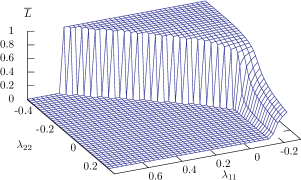
Figure 3: MF behavior of the order parameter $\bar{L}$ for the Ising-type PLA $T_{2}$ from (75).

In FIG. 4 the results for the order parameter $\bar{L}$ as obtained by MC simulations are plotted. Shown is $\bar{L}$ for several thousand sample points in the $(\lambda_{11},\lambda_{22})$ plane. Near the second–order phase transition curve with $\lambda_{11}\lesssim 0.2$ about $2.5$M updates were sufficient, whereas near the transition curve with $\lambda_{11}\gtrsim 0.2$ at least $50$M updates were required.

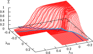
Figure 4: MC data for the order parameter $\bar{L}$ for the Ising-type PLA $T_{2}$ from (75). Shown are the critical curves of the MF approximation (dark) and MC simulations (bright).

We interpret this slow convergence as a signal for a first–order phase transition as predicted by the MF approximation, see FIG. 4.

IV.2 Ginzburg–Landau–type models

Inspired by the nomenclature in Svetitsky (1986) we call effective actions with a nonvanishing potential as in (29) Ginzburg–Landau–type models. The lowest–order potential term is $V_{2}$ given in (35) which is of NLO in the strong–coupling expansion. Hence we first consider the action

$$S_{2}=T_{2}+V_{2},\quad V_{2}=2d\lambda_{02}\sum_{\mbox{\scriptsize\boldmath$x$}}\chi_{2\mbox{\scriptsize\boldmath$x$}}\;.$$ (77)

For $\lambda_{02}\neq 0$ the MF potentials and mean values must be computed numerically. Only for the special case of vanishing source may the relevant integrals be found analytically,

$$\int\!dh(u)\,e^{-2au^{2}}\chi_{2p}(u)=\frac{(-)^{p}}{e^{a}}\left[I_{p}(a)+I_{p+1}(a)\right]\;.$$ (78)

For what follows it is useful to define

$$s_{pq} = I_{p}(4d\lambda_{02})+I_{q}(4d\lambda_{02})\;,$$ (79)

$$d_{pq} = I_{p}(4d\lambda_{02})-I_{q}(4d\lambda_{02})\;,$$ (80)

so that the mean characters can be written as

$$\langle\chi_{2p}\rangle\big{|}_{j=0}=(-)^{p}\;\frac{s_{p,p+1}}{s_{01}}\;.$$ (81)

Using (79) and (80) the critical surface for second–order transitions in the $3$-dimensional space of coupling constants $\lambda_{11},\lambda_{22},\lambda_{02}$ is determined by the equation

$$\lambda_{11}=-\frac{1}{2d}\frac{s_{01}}{d_{02}}+\lambda_{22}\left(\frac{s_{12}}{d_{02}}\right)^{2}\left(\frac{s_{03}}{s_{12}}-\frac{s_{12}}{s_{01}}\right)\;,$$ (82)

which is plotted in FIG. 5.

Figure 5: Critical surface for the Ginzburg–Landau PLA $S_{2}$ from (77).

The NNLO Ginzburg–Landau–type model is given by

$$S_{3}=T_{3}+V_{3}\;,$$ (83)

and has the same potential $V_{3}=V_{2}$ as the NLO action (77) whence (81) still holds. It follows that the critical surface for second–order transitions in the $5$-dimensional space of coupling constants $\lambda_{11},\lambda_{22},\lambda_{02},\lambda_{13},\lambda_{33}$ is determined by the transcendental equation

$$\lambda_{11} = -\frac{1}{2d}\frac{s_{01}}{d_{02}}+\lambda_{22}\left(\frac{s_{12}}{d_{02}}\right)^{2}\left(\frac{s_{03}}{s_{12}}-\frac{s_{12}}{s_{01}}\right)$$ (84)

$$-\lambda_{33}\left(\frac{d_{12}}{d_{02}}\right)^{2}+2\lambda_{13}\frac{d_{12}}{d_{02}}\;.$$

For fixed small couplings $\lambda_{33}$ and $\lambda_{13}$ this surface is very close to the one in FIG. 5.

Summarizing we have seen that the effective models undergo both first– and second–order phase transitions, and that an MF prediction for the phase structure of these models agrees well with the results of MC simulations.

V IMC Results for $\bm{\lambda_{pq}(\beta)}$

Employing our IMC method based on the geometrical Schwinger–Dyson equations of Section II we have calculated the couplings $\lambda_{pq}$ for different PLAs as functions of $\beta$. For our lattice with $N_{s}=20$ and $N_{t}=4$ the critical Wilson coupling is $\beta_{c}=2.30$. Below $\beta_{c}$ we find the hierarchy

$$|\lambda_{11}|\gg|\lambda_{22}|\,,\;|\lambda_{02}|\gg|\lambda_{33}|\,,\;|\lambda_{13}|\;,$$ (85)

in agreement with the strong–coupling expansion (21-23). According to Ogilvie Ogilvie (1984), the weak–coupling asymptotics of $\lambda_{11}$ is linear in $\beta$,

$$\lambda_{11}(\beta)=-\frac{\beta}{2N_{C}N_{t}}+\hbox{const}\quad(\beta\gg\beta_{c})\;,$$

which in our case ($N_{C}=2$) leads to

$$\lambda_{11}(\beta)=-\frac{\beta}{16}+\hbox{const}=-0.0625\,\beta+\hbox{const}\;.$$ (86)

We have compared our IMC results for the couplings $\lambda_{pq}(\beta)$ with the strong–coupling predictions (17, 24-27) and the weak–coupling result (86). As expected from our reasoning above, the lowest order PLAs based on group characters approximate the true Polyakov–loop dynamics very well in the strong–coupling regime. For weak coupling we find the linear relation (86) already for the LO PLA. For the NLO Ginzburg–Landau–type model with $3$ couplings the slope $-0.0614$ is very close to the weak coupling result $-0.0625$ in (86). Thus we are confident that our PLAs describe the true Polyakov loop dynamics below and above the critical Wilson coupling very well.

V.1 Leading–order action

The effective couplings $\lambda_{11}$ for the LO Ising–type model (70) for $\beta$–values below and above the critical $\beta_{c}=2.30$ are listed in TABLE 6, Appendix A. We read off the value $\lambda_{11}(\beta_{c})=-0.132$. If $S_{1}$ would be the exact PLA then its critical coupling $\lambda_{11c}$ would be $\lambda_{11}(\beta_{c})$. A direct MC simulation of the action $S_{1}$ reveals that this model has critical coupling $\lambda_{11c}=-0.18$. The MF prediction $\lambda_{11c}=-0.17$ comes surprisingly close to the former ‘true’ value. The critical coupling may alternatively be estimated by using the strong–coupling results (18) and (24) to calculate $\lambda_{11}(\beta_{c})$ (extrapolating them to $N_{t}=4$ and $\beta_{c}=2.30$),

$$\lambda_{11}=-(\beta/4)^{N_{t}}\stackrel{{\scriptstyle\beta=\beta_{c}}}{{\approx}}-0.11\;.$$ (87)

The output of the different methods is compiled in TABLE 1.

Table 1: Comparison of the critical coupling values for the LO Ising–type model $S_{1}$. The ‘exact’ value is obtained via MC simulation.

method	critical coupling
MC simulation	$\lambda_{11c}=-0.18$
MF	$\lambda_{11c}=-0.17$
strong coupling	$\lambda_{11c}=-0.11$
IMC	$\lambda_{11}(\beta_{c})=-0.14$

The values obtained are quite close to each other. The ‘true’ value $-0.18$ stems from simulating (70) with the MF approximation coming closest. Somewhat surprisingly, the strong–coupling result yields the right order of magnitude. The discrepancy between direct simulation and IMC just means that the action (70) represents an oversimplification and does not match with Yang–Mills well enough. The IMC value $\lambda_{11}(\beta_{c})=-0.14$ constitutes a compromise equivalent to a one–parameter fit of the effective to the Yang–Mills Schwinger–Dyson equations or $n$–point functions.

In FIG. 6 we compare the results for $\lambda_{11}$ from strong– and weak–coupling expansion with the data of our IMC simulations. Note that the asymptotic formula (87) works up to $\beta\simeq 2$. The IMC values for the LO action $S_{1}$ in (70) are marked with circles.

Figure 6: The coupling $\lambda_{11}$ as a function of $\beta$. Dashed curve for $\beta<\beta_{c}$: asymptotic behavior (87); dashed lines for $\beta>\beta_{c}$: linear fits $\lambda=a\beta+b$; data points: IMC results from Tables 6-8 in Appendix A.

Note further that the dependence $\lambda_{11}(\beta)$ is indeed linear in the weak–coupling regime, $\lambda_{11}=-0.0392\,\beta-0.0774$, in accordance with the prediction (86) for the weak–coupling asymptotics. The slope, however, turns out being too small. This will be remedied in what follows by including more couplings.

V.2 Next–to–leading–order actions

The effective action (70) has been confirmed and extended by several authors Ogilvie (1984); Drouffe et al. (1984); Green and Karsch (1984); Gross and Wheater (1984). We have also checked its generalizations by considering the NLO Ising–type model (75) without potential terms and the Ginzburg–Landau action (77) containing all NLO terms from (33).

The NLO IMC results for $\lambda_{11}(\beta)$ are displayed in FIG. 6 (crosses and asterisks), those for $\lambda_{22}(\beta)$ in FIG. 7 (same symbols) and those for $\lambda_{02}(\beta)$ in FIG. 8 (asterisks). The error bars for the couplings are listed in the tables in Appendix A. Upon comparing the values for $\lambda_{11}$ in FIG. 6 (or TABLE 6) we note that for $\beta<\beta_{c}$ the predictions for $\lambda_{11}$ are almost model independent. In the weak–coupling regime, on the other hand, they are less stable. Hence, adding terms to the PLA may change the coupling constants considerably in this regime.

For the NLO actions the dependence $\lambda_{11}(\beta)$ is linear in the weak coupling regime, similarly as for the LO action $S_{1}$. However, the slopes $a$ in the linear fits $\lambda_{11}(\beta)=a\beta+b$ above $\beta_{c}$ are model dependent. For the LO and NLO PLA they are given in TABLE 2 together with the weak–coupling result (86).

Table 2: Slopes of the linear fits to the weak–coupling asymptotics (V) of $\lambda_{11}$.

model	$1/2N_{C}N_{t}$	$S_{1}$	$T_{2}$	$S_{2}$
slope	-0.0625	-0.0392	-0.0505	-0.0614

For the Ising–type models without potential terms the slope is not reproduced very well, and we conclude that in the weak–coupling or high–temperature regime potential terms should be included for an accurate description of the Polyakov–loop dynamics. Indeed, the slope for the action (77) with potential term $V_{2}$ is almost identical to the prediction (V) of the weak–coupling asymptotics.

FIG. 7 shows the dependence of the adjoint coupling constant $\lambda_{22}$ on the Wilson coupling $\beta$. Also shown is the prediction (25) of the strong coupling expansion using (18),

$$\lambda_{22}(\beta)=-\frac{113}{162}\left({\beta\over 4}\right)^{8}\approx-0.69753\left({\beta\over 4}\right)^{8}\;,$$ (88)

which again reproduces the IMC results for $\beta<2$.

Figure 7: The adjoint coupling $\lambda_{22}$ as a function of $\beta$ for the NLO and NNLO actions. Dashed curve: asymptotic behavior (88); data points: IMC results from Tables 6-8.

The critical coupling

$$\lambda_{22}(\beta_{c})=-0.008[1]$$ (89)

is the same for both PLAs (70) and (77). Up to $\beta_{c}$ the two actions have almost identical couplings $\lambda_{22}$. It seems that for $\beta>\beta_{c}$ these couplings also depend linearly on $\beta$, as was the case for $\lambda_{11}(\beta)$.

Figure 8: The coupling $\lambda_{02}$ as a function of the Wilson coupling $\beta$ for NLO, NNLO and Ginzburg–Landau actions; data points: IMC results from Tables 7-9.

V.3 Next-to-next-to-leading order

We have seen that the NLO approximations describe the Polyakov loop dynamics very well in the symmetric strong–coupling phase. In the weak–coupling regime, however, there is still room for improvement. Hence we have calculated the five coupling constants $\lambda_{11},\lambda_{22},\lambda_{02},\lambda_{13},\lambda_{33}$ appearing in the general NNLO PLA $S_{3}$ for several values of the Wilson coupling. This action is the sum of all terms up to order $\beta_{t}^{\,3N_{t}}$ in the strong–coupling expansion. As expected, adding the third order terms $S_{31}$ and $S_{33}$ does not change the lower–order couplings $\lambda_{11},\lambda_{22},\lambda_{02}$ (as obtained via $S_{2}$) in the broken phase. This can be seen in FIG.s 6, 7 and 8, where the IMC results for the NNLO action $S_{3}$ from (34) are depicted by triangles. The numerical values for these couplings and the couplings $\lambda_{33}$ and $\lambda_{13}$ together with their statistical errors are given in Appendix A.

V.4 Ginzburg–Landau models

In his review Svetitsky (1986), Svetitsky has suggested to emphasize the potential term in (3) by specializing to an ansatz of Ginzburg–Landau type,

$$S_{\mathrm{GL}}=S_{1}+\sum_{\mbox{\scriptsize\boldmath$x$}}V(L_{\mbox{\scriptsize\boldmath$x$}})\;,$$ (90)

with center–symmetric potential (30). Replacing the coefficients $\lambda_{0p}$ of the characters in this potential by

$$\lambda_{4} = 2d\cdot 4^{2}\lambda_{04}\;,$$ (91)

$$\lambda_{2} = 2d\cdot 4(\lambda_{02}-3\lambda_{04})\;,$$ (92)

leads for $p\leq 4$ to the even polynomial

$$V(L)=\lambda_{2}L^{2}+\lambda_{4}L^{4}+\rm{const}\;.$$ (93)

In Table 9 we have listed the couplings for the models with quadratic and quartic potentials,

$$S^{(1)}_{\mathrm{GL}} = S_{1}+\lambda_{2}\sum_{\mbox{\scriptsize\boldmath$x$}}L_{\mbox{\scriptsize\boldmath$x$}}^{2}\;,$$ (94)

$$S^{(2)}_{\mathrm{GL}} = S_{\mathrm{GL}}^{(1)}+\lambda_{4}\sum_{\mbox{\scriptsize\boldmath$x$}}L_{\mbox{\scriptsize\boldmath$x$}}^{4}\;,$$ (95)

obtained via IMC within our standard range of $\beta$. The values for $\lambda_{11}$ both for strong and weak coupling are almost identical to those of the NLO model $S_{2}$. For this reason we have refrained from plotting them in FIG. 6. The potential couplings are important in the broken weak–coupling phase where they become sizable. The coupling $\lambda_{02}$ for the Ginzburg–Landau models (94,95) is shown in FIG. 8.

V.5 Summary

The values for the couplings of the different PLAs arising at critical Wilson coupling $\beta_{c}=2.30$ are listed in TABLE 3. They are almost model independent. $\lambda_{11}$, in particular, is always close to the MF value $-0.167$ (for the Ising type models).

Table 3: Effective couplings of different PLAs at $\beta=\beta_{c}=2.30$.

model	$S_{1}$	$T_{2}$	$S_{2}$	$S_{3}$	$S_{\mathrm{GL}}^{(2)}$
$\lambda_{11}(\beta_{c})$	$-0.133$	$-0.135$	$-0.156$	$-0.156$	$-0.155$
$\lambda_{22}(\beta_{c})$		$0.006$	$0.006$	$0.006$
$\lambda_{02}(\beta_{c})$			0.011	$0.012$	$0.012$

The couplings below and above $\beta_{c}$ and their statistical errors are compiled in Appendix A. There one may also find $\lambda_{33},\lambda_{13}$ and $\lambda_{04}=\lambda_{4}/32d$ for different Wilson couplings.

The stability of the couplings for $\beta<\beta_{c}$ is a strong indication that (in this regime) the Yang–Mills ensemble is very well approximated already by the NLO models with $2$ or $3$ couplings. The results of the following section will further confirm this statement.

The Ising–type coupling $\lambda_{11}$ becomes a linear function of $\beta$ in the weak–coupling regime, in accordance with the weak–coupling prediction (V). For the NLO action the slope is $-0.0614$ which compares favorably with the weak–coupling value $-0.0625$. For the Ginzburg–Landau–type actions the slope is almost identical to the one of the NLO models.

The Ising–type couplings change rapidly at the critical Wilson coupling $\beta_{c}=2.30$ as demonstrated in FIG.s 6 and 7. For example, the coupling $\lambda_{11}$ decreases from $-0.1$ below $\beta_{c}$ to $-0.2$ above $\beta_{c}$. This jump of $\lambda_{11}$ forces the system into the ferromagnetic phase. For $\lambda_{22}$ the jump is even more dramatic, from $0$ to $0.04$. The potential couplings $\lambda_{02}$ and $\lambda_{04}$ change more smoothly when the systems changes from the symmetric to the broken phase.

VI Two–point functions

Let us finally check the quality of our PLAs which, after all, should represent approximations to Yang–Mills theory. To this end we compare the Yang–Mills two–point function at different $\beta$–values with those of our effective models inserting the couplings $\lambda_{pq}(\beta)$ obtained via IMC. For the NLO actions at $\beta=2.2$ these couplings are displayed in TABLE 4,

Table 4: Effective couplings for NLO actions at $\beta=2.2$.

$\beta=2.2$	$\lambda_{11}$	$\lambda_{22}$	$\lambda_{20}$
$T_{2}$	0.1033	0.0019
$S_{2}$	0.1168	0.00042	0.0064

while for $\beta=3.0$ we have the NLO and NNLO couplings of TABLE 5.

Table 5: Effective couplings for NLO and NNLO actions at $\beta=3.0$.

$\beta=3$	$\lambda_{11}$	$\lambda_{22}$	$\lambda_{20}$	$\lambda_{33}$	$\lambda_{31}$
$T_{2}$	0.2207	0.0320
$S_{2}$	0.2361	0.0194	0.0165
$S_{3}$	0.2506	0.0311	0.0236	0.0035	0.0040

With these couplings we have simulated the models with actions

$$T_{2}\,,\quad S_{2}\,,\quad S_{3}\,,\quad S_{\rm GL}^{(1)}\,,\quad S_{\rm GL}^{(2)}\,,$$ (96)

and calculated the two–point functions displayed in FIG.s 9 and 10. As expected, the agreement in the center–symmetric phase ($\beta=2.2$) is very good, while deep in the broken phase ($\beta=3.0$) there appears to be room for improvement.

Figure 9: The Yang–Mills (YM) two–point function compared to the ones obtained from the NLO effective actions $T_{2}$ and $S_{2}$; $(N_{s},N_{t})=(20,4)$.

For $\beta=2.2$ the two–point functions of the three effective models considered are almost identical to the Yang–Mills two–point function. The data points for $S_{3}$ and $S^{(2)}_{\rm GL}$ cannot be distinguished from those for the NLO model $S_{2}$ and hence are not displayed in FIG. 9.

For $\beta=3.0$ the two–point functions and the expectation value of the mean field are model dependent. In FIG. 10 we have plotted the two–point function of Yang–Mills theory and of the NLO and NNLO effective actions.

For the NLO approximation $T_{2}$ the value for the condensate is approximately 20 percent below the Yang–Mills value. Including potential terms ($S_{2}$) and NNLO terms ($S_{3}$) improves the approximation somewhat as FIG. 10 shows. The two–point function for the Ginzburg–Landau action $S^{(2)}_{\rm GL}$ is almost identical to the one of $T_{2}$ (and thus has not been displayed). This implies that also higher–order Ising (or hopping) terms are important when $\beta>\beta_{c}$.

Figure 10: The Yang–Mills (YM) two–point function compared to the one obtained from the NLO ($T_{2}$ and $S_{2}$) and NNLO ($S_{3}$) effective actions; $(N_{s},N_{t})=(20,4)$.

VII Discussion

To really obtain satisfactory approximations to Yang–Mills expectation values (e.g. two–point functions) for all $\beta$–values one has to go beyond nearest–neighbor interactions in the effective theory. This has been done in Dittmann et al. (2004) where operators with $r\equiv|\mbox{\boldmath$x$}-\mbox{\boldmath$y$}|$ up to $\sqrt{2}$ (‘plaquette operators’) were included. We briefly recapitulate the results of this brute–force calculation. By reformulating the Schwinger–Dyson equations (12) in terms of characters, the couplings have been determined by our standard inverse Monte–Carlo routines. We found that the couplings decrease rapidly not only if we go to higher representations (i.e. larger $p$) as above, but also if we increase the number of links within the plaquette operators used. The leading $r=1$ term $S_{1}$ of (32) with coupling $\lambda_{11}$ dominates by one order of magnitude compared to the terms with $r=\sqrt{2}$. This clearly indicates that the effective interactions are short–ranged in accordance with the Svetitsky–Yaffe conjecture. Simulating the effective action including plaquette operators with the couplings obtained via IMC we have calculated the two–point function in both phases. Including a total of $14$ couplings the matching between Yang–Mills and the effective action becomes perfect both in the broken and symmetric phase Dittmann et al. (2004). It should, however, be stressed that this brute–force numerical calculation does not provide too much of physical intuition. We believe that the present paper, in particular the mean–field analysis, improves upon Dittmann et al. (2004) in this respect.

The most straightforward generalization of our analysis obviously is to go to $SU(3)$ Yang–Mills theory where one expects a first order phase transition. Work in this direction is under way.

Appendix A Tables

The following TABLEs 6–9 contain the effective couplings $\lambda_{pq}$ with statistical errors for various values of $\beta$.

Table 6: IMC results for the effective coupling $\lambda_{11}$ in the LO action $S_{1}$ and the two couplings $\lambda_{11},\lambda_{22}$ in $T_{2}$.

Yang-Mills-$\beta$	$S_{1}:\lambda_{11}$	$T_{2}:\lambda_{11}$	$T_{2}:\lambda_{22}$
1.70	-0.0305[4]	-0.030[2]	-0.001[1]
2.20	-0.1040[2]	-0.103[1]	-0.0019[7]
2.28	-0.1231[3]	-0.123[1]	0.000[1]
2.29	-0.1267[4]	-0.127[1]	0.002[1]
2.30	-0.1325[5]	0.135[1]	0.006[1]
2.32	-0.1512[3]	-0.1598[9]	0.023[1]
2.34	-0.1585[2]	-0.1697[6]	0.030[1]
2.38	-0.1658[1]	-0.1799[4]	0.037[1]
2.60	-0.1792[1]	-0.1989[4]	0.0382[8]
2.80	-0.1874[1]	-0.2103[5]	0.0350[8]
3.00	-0.1952[1]	-0.2206[6]	0.0319[8]
3.50	-0.2146[1]	-0.2446[6]	0.0264[6]
4.00	-0.2343[1]	-0.2670[9]	0.0225[6]

Table 7: IMC results for the three couplings in $S_{2}$.

$\beta$	$\lambda_{11}$	$\lambda_{22}$	$\lambda_{20}$
1.10	-0.004[4]	-0.000[2]	-0.0012[5]
1.70	-0.030[4]	-0.001[2]	-0.0007[5]
2.20	-0.116[2]	0.000[2]	0.0064[5]
2.28	-0.144[2]	0.002[2]	0.0101[5]
2.29	-0.148[2]	0.004[2]	0.0108[5]
2.30	-0.156[2]	0.006[2]	0.0114[5]
2.32	-0.178[2]	0.017[2]	0.0125[6]
2.34	-0.187[1]	0.022[2]	0.0130[6]
2.38	-0.195[1]	0.026[2]	0.0130[6]
2.60	-0.212[1]	0.026[2]	0.013[1]
2.80	-0.224[1]	0.022[2]	0.014[1]
3.00	-0.236[1]	0.019[2]	0.016[1]
3.50	-0.267[1]	0.010[2]	0.025[1]
4.00	-0.299[1]	0.003[2]	0.037[1]

Table 8: IMC results for five couplings in $S_{3}$.

$\beta$	$\lambda_{11}$	$\lambda_{22}$	$\lambda_{20}$	$\lambda_{33}$	$\lambda_{31}$
1.10	-0.004[1]	0.000[1]	-0.0011[2]	0.000[1]	0.0003[6]
1.70	-0.029[2]	0.000[1]	-0.0006[2]	0.0001[8]	0.0000[6]
2.20	-0.116[1]	0.000[1]	0.0064[2]	0.0015[7]	0.0000[6]
2.28	-0.143[1]	0.002[1]	0.0102[3]	0.0015[8]	0.0002[6]
2.29	-0.148[1]	0.003[1]	0.0108[3]	0.0015[8]	0.0000[6]
2.30	-0.156[1]	0.006[1]	0.0115[3]	0.001[1]	0.0000[6]
2.32	-0.179[1]	0.019[1]	0.0129[3]	-0.0006[9]	-0.0004[5]
2.34	-0.1892[8]	0.026[1]	0.0138[3]	-0.0014[8]	-0.0014[6]
2.38	-0.1999[6]	0.035[1]	0.0148[4]	-0.0032[9]	-0.0026[5]
2.60	-0.2227[8]	0.040[1]	0.0176[5]	-0.005[1]	-0.0041[4]
2.80	-0.236[1]	0.035[1]	0.0202[8]	-0.0041[9]	-0.0040[4]
3.00	-0.250[1]	0.031[1]	0.0235[8]	-0.0034[8]	-0.0039[4]
3.50	-0.283[1]	0.020[1]	0.032[1]	-0.002[1]	-0.0032[6]
4.00	-0.291[3]	0.003[1]	0.029[2]	-0.0033[9]	0.0029[8]

Table 9: IMC results for the couplings $\lambda_{11},\lambda_{2},\lambda_{4}$ in $S^{(2)}_{\rm GL}$.

$\beta$	$\lambda_{11}$	$\lambda_{2}$	$\lambda_{4}$
2.20	-0.110	0.186	-0.002
2.25	-0.119	0.237	-0.003
2.28	-0.127	0.288	-0.006
2.29	-0.128	0.303	-0.007
2.30	-0.157	0.453	-0.020
2.32	-0.173	0.621	-0.057
2.34	-0.176	0.698	-0.093
2.40	-0.190	0.979	-0.256

Appendix B Numerical Details

All MC calculations have been performed on a $20^{3}\times 4$ lattice for which the critical Wilson coupling is $\beta_{c}=2.30$. The simulations have been done for $\beta$ ranging from 1.1 to 4.0. We have used a standard ‘pseudo-heatbath’ algorithm Kenedy and Pendleton (1985); Fabricius and Haan (1984) due to Miller Miller (2001).

The IMC routine has been implemented as follows. For each action term $S_{pq}$ and site we have chosen the operator

$$G_{pq,\mbox{\scriptsize\boldmath$z$}}\equiv\frac{1}{\lambda_{pq}}\frac{\delta S_{pq}}{\delta L_{\mbox{\scriptsize\boldmath$z$}}}\;,$$ (97)

which leads to the Schwinger–Dyson equations

$$\sum_{(pq)}\lambda_{pq}\langle(1\!-\!L_{\mbox{\scriptsize\boldmath$x$}}^{2})G_{pq,\mbox{\scriptsize\boldmath$z$}}S_{pq,\mbox{\scriptsize\boldmath$x$}}\rangle=\langle(1\!-\!L_{\mbox{\scriptsize\boldmath$x$}}^{2})G_{,\mbox{\scriptsize\boldmath$x$}}-3L_{\mbox{\scriptsize\boldmath$x$}}G\rangle\;.$$ (98)

Due to translational invariance the coefficients of $G_{\mbox{\scriptsize\boldmath$z$}}$ and $G_{\mbox{\scriptsize\boldmath$z$}^{\prime}}$ are equal if $|\mbox{\boldmath$x$}-\mbox{\boldmath$z$}|=|\mbox{\boldmath$x$}-\mbox{\boldmath$z$}^{\prime}|$. In order to have a sufficiently overdetermined system (for fixed $pq$) we choose the $N_{s}$ operators $G_{pq,d}$, $d=0\ldots N_{s}$. Independent of our choice of PLA we have always used the full set of operators up to truncation values $p,q=5$, i.e.

$$G_{11},G_{22},G_{20},G_{33},G_{31},G_{44},G_{42},G_{40},G_{55}$$ (99)

with $0\leq d\leq 8$ leading to a total of 81 operators (and equations). Translational invariance admits to use the spatial average of each Schwinger–Dyson equation and every configuration. The overdetermined system is then solved via least–square methods. We have checked that the couplings obtained in this way follow a normal distribution, as expected. Hence we calculated the standard deviation $\sigma$ and took $2\sigma$ as our error. Autocorrelation effects have been eliminated via binning. Our statistics (5k to 10k configurations) entail a statistical error of $10^{-4}$ which translates into an uncertainty for the couplings in the NLO action of the order of a few percent. The NNLO couplings $\lambda_{33}$ and $\lambda_{31}$, however, have statistical errors of about $20\%$.

Systematic errors are mainly due to the dependence of the couplings on the operator bases used in the Schwinger–Dyson equations.

References

• (1)
• Polyakov (1978) A. M. Polyakov, Phys. Lett. B72, 477 (1978).
• Susskind (1979) L. Susskind, Phys. Rev. D20, 2610 (1979).
• Caselle and Hasenbusch (1996) M. Caselle and M. Hasenbusch, Nucl. Phys. B470, 435 (1996), eprint hep-lat/9511015.
• Gliozzi and Provero (1997) F. Gliozzi and P. Provero, Phys. Rev. D56, 1131 (1997), eprint hep-lat/9701014.
• de Forcrand and von Smekal (2003) P. de Forcrand and L. von Smekal, Phys. Rev. D66, 011504 (2002), eprint hep-lat/0107018.
• Pepe and de Forcrand (2002) M. Pepe and P. de Forcrand, Nucl. Phys. B (Proc. Suppl.) 106, 914 (2002), eprint hep-lat/0110119.
• Svetitsky and Yaffe (1982) B. Svetitsky and L. Yaffe, Nucl. Phys. B210, 423 (1982).
• Yaffe and Svetitsky (1982) L. G. Yaffe and B. Svetitsky, Phys. Rev. D26, 963 (1982).
• Svetitsky (1986) B. Svetitsky, Phys. Rept. 132, 1 (1986).
• Falcioni et al. (1986) M. Falcioni, G. Martinelli, M. Paciello, G. Parisi, and B. Taglienti, Nucl. Phys. B265, 187 (1986).
• Gonzalez-Arroyo and Okawa (1987) A. Gonzalez-Arroyo and M. Okawa, Phys. Rev. D 35, 672 (1987).
• Banks (2004) T. Banks (2004), eprint hep-th/0412129.
• Meisinger et al. (2002) P. Meisinger, T. Miller, and M. Ogilvie, Phys. Rev. D65, 034009 (2002).
• Dumitru et al. (2004) A. Dumitru, Y. Hatta, J. Lenaghan, K. Orginos, and R. D. Pisarski, Phys. Rev. D70, 034511 (2004), eprint hep-th/0311223.
• Dittmann et al. (2004) L. Dittmann, T. Heinzl, and A. Wipf, JHEP 06, 005 (2004), eprint hep-lat/0306032.
• Billó et al. (1996) M. Billó, M. Caselle, A. D’Adda, and S. Panzeri, Nucl. Phys. B472, 163 (1996), eprint [http://arXiv.org/abs]hep-lat/9601020.
• Abramowitz and Stegun (1964) M. Abramowitz and I. Stegun, eds., Handbook of Mathematical Functions (National Bureau of Standards, 1964).
• Roepstorff (1994) G. Roepstorff, Path Integral Approach to Quantum Physics (Springer, 1994).
• Fujimoto et al. (1988) Y. Fujimoto, H. Yoneyama, and A. Wipf, Phys. Rev. D38, 2625 (1988).
• O’Raifeartaigh et al. (1986) L. O’Raifeartaigh, A. Wipf, and H. Yoneyama, Nucl. Phys. B271, 653 (1986).
• Polónyi and Szlachányi (1982) J. Polónyi and K. Szlachányi, Phys. Lett. B110, 395 (1982).
• Ogilvie (1984) M. Ogilvie, Phys. Rev. Lett. 52, 1369 (1984).
• Drouffe et al. (1984) J. Drouffe, J. Jurkiewicz, and A. Krzywiecki, Phys. Rev. D29, 2982 (1984).
• Green and Karsch (1984) F. Green and F. Karsch, Nucl. Phys. B238, 297 (1984).
• Gross and Wheater (1984) M. Gross and J. Wheater, Nucl. Phys. B240, 253 (1984).
• Kenedy and Pendleton (1985) A. Kenedy and B. Pendleton, Phys. Lett.B 156, 393 (1985).
• Fabricius and Haan (1984) K. Fabricius and O. Haan, Phys. Lett. B 143, 459 (1984).
• Miller (2001) T. R. Miller (2001), available at URL http://hbar.wustl.edu/ miller/howto.html.