The compact $Q=2$ Abelian Higgs model in the London limit:
vortex–monopole chains and the photon propagator

Abstract

The confining and topological properties of the compact Abelian Higgs model with doubly–charged Higgs field in three space-time dimensions are studied. We consider the London limit of the model. We show that the monopoles are forming chain-like structures (kept together by ANO vortices) the presence of which is essential for getting simultaneously permanent confinement of singly–charged particles and breaking of the string spanned between doubly–charged particles. In the confinement phase the chains are forming percolating clusters while in the deconfinement (Higgs) phase the chains are of finite size. The described picture is in close analogy with the synthesis of the Abelian monopole and the center vortex pictures in confining non–Abelian gauge models. The screening properties of the vacuum are studied by means of the photon propagator in the Landau gauge.

I Introduction

The Abelian Higgs model with compact gauge fields (cAHM) has potential applications in various areas of physics. Examples range from high energy physics ref:HEP ; Bhanot:1981ug over condensed matter physics ref:CondMatt ; ref:Kleinert to neural networks ref:Neural etc. Recently a closer relation of this model to the infrared sector of the theory of strong interaction (QCD) was discussed ref:U1Q2PLB . The model is also interesting by itself due to its non–perturbative features which can be treated analytically in some cases.

The non–perturbative features of the cAHM arise due to presence of topological defects among the excitations of the model. There are two types of defects: monopoles and Abrikosov-Nielsen-Olesen (ANO) vortices ANO . The monopoles appear due to the compactness of the gauge vector field while the existence of vortices is linked to the compactness of the phase of the Higgs field. Vortices carry magnetic flux which begins/ends on monopoles/antimonopoles.

The study of the cAHM with doubly–charged Higgs field ($Q=2$ cAHM) presented below is motivated by the relation of this model to gluodynamics. In the confinement phase of the $Q=2$ cAHM the singly–charged external particles must be confined by a linear potential while the potential between external doubly–charged particles should flatten at large separation between the charges due to the so-called string-breaking phenomenon. This feature makes $Q=2$ cAHM similar to gluodynamics in which the fundamental charged (static quarks) are confined while the potential between the adjoint charges (static “gluons”) is asymptotically screened.

The different effect on singly– and doubly–charged external particles can be reconciled ref:U1Q2PLB with monopole dynamics only if one assumes that monopoles are bound into chains which occupy the whole volume of the lattice. Indeed, the monopole gas is known ref:Polyakov to be confining at all distances, and no string breaking and, consequently, the flattening of the potential is possible. As a relevant physical example one may cite the compact $U(1)$ gauge model without matter fields (i.e. in compact electrodynamics, cQED₃) at zero temperature where the monopoles form a Coulomb plasma ref:Polyakov .

The other extreme, the vacuum filled only by a gas of monopole–anti-monopole bound pairs, cannot be confining at all FrSp80 . This situation is realized in cQED₃ at high temperatures ref:cQED:Binding as well as in cAHM with singly–charged dynamical matter fields ref:Kleinert ; Chernodub:2002ym .

Therefore, in the case of $Q=2$ cAHM, the monopoles must form structures different both from the monopole gas and the magnetically neutral dipole gas. In fact, it was found numerically ref:U1Q2PLB that in the presence of a doubly–charged Higgs field the monopoles actually form chain–like structures. This offers an explanation of both confinement of singly–charged electric particles and string breaking for doubly–charged test particles.

The described pattern of charge confinement in $Q=2$ cAHM has a close analogy with gluodynamics where tight correlations between Abelian monopoles and center vortices (each in the respective Abelian projection ) have been found Greensite_3 . It also suggests a natural mechanism for the formation of monopole sheets (instead of chains in 3D) in 4D gluodynamics. For example, in the pure SU(2) gauge model (chosen here for simplicity of discussion) the Abelian monopoles are defined with the help of an Abelian gauge, in which the off-diagonal gluons (originally ignored in the Abelian projection) play the role of the doubly–charged matter fields coupled minimally to the leading diagonal gluons. The presence of the doubly–charged dynamical matter leads to the formation of the vortices carrying magnetic flux ref:GubarevAHM . These “magnetic” vortices are similar to center vortices. The off-diagonal matter fields also may cause, as pointed out in Ref. ref:U1Q2PLB , the monopole trajectories to be confined inside sheets.

In this paper we complete the study of the cAHM in three space-time dimensions along the direction outlined in Ref. ref:U1Q2PLB , restricting ourselves to the London limit. We hope to come back to the model at finite quartic Higgs coupling on another occasion. We study the structure of the monopole chains, vortex and monopole cluster properties at various couplings of the $Q=2$ cAHM model. The (Debye) screening properties of the vacuum are investigated with the help of the photon propagator.

The structure of this paper is as follows. In Section II we describe general properties of the model on the lattice. In this Section we also discuss the monopole and vortex structures and derive their interactions by rewriting the partition function using the Villain form of the model in the London limit. The topological nature of the confining properties of the model is pointed out. In Section III we numerically investigate the phase structure and the percolation properties of the monopole chains using the model with the cosine form of the action. Both finite and zero temperatures cases are studied. In Section IV we numerically investigate the photon propagator in Landau gauge crossing the phase transition from the confined to the Higgs phase. Our conclusions are discussed in Section V.

II The model

II.1 Lattice formulation

We consider the three-dimensional Abelian Higgs model with compact gauge fields $\theta_{x,\mu}\in[-\pi,\pi)$ which are defined on links $\{x,\mu\}$. Let the scalar Higgs field, $\Phi_{x}\in\mathbb{C}$, be doubly–charged and written in the form

$$\Phi_{x}=\rho_{x}{\rm e}^{i\varphi_{x}}$$ (1)

where $\rho_{x}$ is its modulus (radial part) and $\varphi_{x}$ its phase. The action of the model is

$$S=-\beta\sum_{P}\cos\theta_{P}-\kappa\sum_{x,\mu}\rho_{x}\rho_{x+\hat{\mu}}\cos(-\varphi_{x}-2\,\theta_{x,\mu}+\varphi_{x+\hat{\mu}})+\sum_{x}(\rho_{x}^{2}+\lambda(\rho_{x}^{2}-1)^{2})\,,$$ (2)

where $\theta_{P}$ is the plaquette angle. The parameter $\beta$ is proportional to the inverse gauge coupling squared, $\beta=1/(a\,g^{2})$, $\kappa$ is the so-called hopping parameter and $\lambda$ the quartic Higgs self coupling.

In a special limit of the model – the so-called “London limit” – the coupling $\lambda$ is infinite and therefore the radial mode of the Higgs field is frozen to unity. In this paper we study this limit in detail and relegate the more general case of the radially active model to another paper. In the London limit Eq. (2) reduces to

$$S_{\rm London}[\theta]=-\beta\sum_{P}\cos\theta_{P}-\kappa\sum_{x,\mu}\cos(-\varphi_{x}-2\,\theta_{x,\mu}+\varphi_{x+\hat{\mu}})\,.$$ (3)

The phase structure of the reduced model can be sketched starting from the following considerations ref:HEP ; Bhanot:1981ug . At vanishing hopping parameter, $\kappa=0$, the model (3) reduces to the pure compact Abelian gauge theory. On the symmetric lattices this model is confining at any coupling $\beta$ due to the presence of the monopole plasma ref:Polyakov . Thus the low-$\kappa$ region of the phase diagram corresponds to the confining phase (“confining region”). At large values of $\kappa$ (called the “Higgs region”) the model reduces to the ${Z\!\!\!Z}_{2}$ gauge model. Indeed, at very large $\kappa$ we get the constraint $\varphi_{x+\hat{\mu}}-2\,\theta_{x,\mu}-\varphi_{x}=2\pi\,l_{x,\mu}$ with $l_{x,\mu}\in{Z\!\!\!Z}$. However, in the unitary gauge, all $\varphi_{x}=0$, and the above constraint along with the compactness condition for the gauge field, $\theta_{x,\mu}\in[-\pi,\pi)$, gives two possible solutions: $\theta_{x,\mu}=0$ and $\theta_{x,\mu}=\pi$. One can rewrite the model of Eq. (3) in this gauge as the ${Z\!\!\!Z}_{2}$ gauge model for the variables $z_{x,\mu}=e^{i\theta_{x,\mu}}=\pm 1$. The ${Z\!\!\!Z}_{2}$ gauge model in three dimensions has a second order phase transition at the critical coupling $\beta^{{Z\!\!\!Z}_{2}}_{c}\approx 0.7613$ Z2phase . A transition line separates the confinement phase [closer to origin, $(\beta,\kappa)=(0,0)$] from the Higgs phase [closer to the point $(\beta,\kappa)=(\infty,\infty)$].

At zero value of the coupling constant $\beta$ the model is trivial. At large $\beta$ the model reduces to the three dimensional $XY$-model due to the constraint for the plaquette variable, $\theta_{P}=2\pi n_{P}$, with $n_{P}\in{Z\!\!\!Z}$. This constraint is solved in the form $\theta_{x,\mu}=-\chi_{x+\hat{\mu}}+\chi_{x}+2\pi l_{x,\mu}$, where $\chi_{x}\in[-\pi,\pi)$ is a compact scalar field. Then a re-scaling of the spin field $\chi_{x}$ by a factor of 2 gives us the $XY$-model which is known to possess a second order phase transition XYphase at $\kappa^{XY}_{c}=0.45420(2)$ between a symmetric and a Higgs phase. The schematic view of the phase diagram is shown in Figure 1.

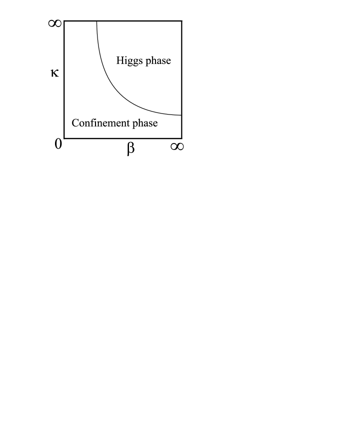
Figure 1: The phase diagram of the 3D Q=2 Abelian Higgs model in the London limit.

From our previous studies in the London limit of the $Q=1$ cAHM at $\beta=2.0$ Chernodub:2002ym we know that there is no transition but the crossover from the “confining region” to the “Higgs region” is signalled by a rapid drop of the monopole density. In addition, a string breaking phenomenon affecting fundamental test charges (being in the same representation as the fundamentally charged matter fields) has been observed in the Higgs region whereas they are bound by a linearly rising (string) potential in the confining region. While the drop of the monopole density signals the onset of deconfinement, the anomalous dimension of the photon propagator is turning to zero at the same crossover $\kappa_{c}(\beta)$. This accompanies the transition from the symmetric/confining to the Higgs region, whereas the observed non-vanishing photon mass at larger $\kappa$ is simply generated by the Higgs effect.

II.2 From $Q=1$ to $Q=2$ and beyond

In the compact U(1) model without dynamical matter fields external static charges $q$ (measured in units of some electric charge $e$) are permanently confined in three space-time dimensions at zero temperature ref:Polyakov . The mechanism is simple: the compact model possesses monopoles which form a Debye plasma state. If the external charges are immersed into this plasma moving around a Wilson loop, monopoles form a sandwich-like structure of magnetic excess charge of opposite sign on both sides of a certain surface. This surface is the minimal area surface spanned by the trajectory of the “electric” charge. The thickness of this structure is of the order of the Debye screening length. This leads to a finite excess free energy per unit area of the double sheet. Thus, oppositely charged external sources at distance $R$ are confined by a linear potential $V_{q}(R)$ due to the monopole plasma.

The situation becomes more complicated when dynamical matter fields with electric charge $Q~{}e$ are present where $Q$ is an integer. In this model – known as the compact Abelian Higgs model (cAHM) – monopoles are not the only topological objects present in the vacuum. The model additionally possesses so called vortices which carry a certain magnetic flux. In the general case the total flux carried by the vortex is $\Phi=2\pi/(Q\,e)$. According to the Dirac quantization condition the monopole carries the charge $m=2\pi/e$. The magnetic flux emitted by an (anti-)monopole is squeezed into the vortices (the Meissner effect). The number of vortices attached to a single (anti)monopole is $Q=m/\Phi$.

If the matter field carries unit charge, $Q=1$, only one vortex is attached to each (anti)monopole. When the vortices possess a non-zero “vortex tension” (i.e. action per length) the monopoles must form monopole–antimonopole pairs (“monopoliums” or, in other words, magnetically neutral dipoles) confined by a linear potential due to the vortex. The monopolium has a characteristic size, $R_{m}$, which is inversely proportional to this vortex tension. This monopole binding changes now the primordial confining potential $V_{q,Q}(R)$ between static external electric charges $q~{}e$.

Firstly, we ignore the Meissner effect and suppose that the vacuum consists of pairs of size $R_{m}$. When the monopolium size is small compared to the distance between the external electric charges, $R_{m}\ll R$, the influence of any monopole on the potential $V_{q,Q}(R)$ is almost compensated by that of an antimonopole belonging to the same pair. Therefore the influence of any (anti-)monopole on the long-distance part of $V_{q,Q}(R)$ is negligibly small and confinement is lost. In other words, a vacuum formed out of dipoles is not confining, so for $R\gg R_{m}$ the potential $V_{q,Q}(R)$ becomes flat. If $R_{m}\gg R$, the field of a single monopole is practically unscreened by the presence of other monopoles. As a consequence, we may expect a piecewise linear potential due to the usual plasma-like mechanism. This picture is exactly the string breaking mechanism. While the string breaking has to appear for external charges of arbitrary strength $q$, the typical string breaking size might depend on $q$. So we conclude, that the binding of the monopoles into magnetically neutral pairs may successfully describe the string breaking in terms of topological degrees of freedom.

The so far neglected Meissner effect provides an additional distance scale, which is equal to the inverse mass of the compact gauge field, $R_{\theta}=1/M_{\theta}$. This scale defines the width of the physical vortex and also the characteristic distance at which the magnetic field of the monopole deviates from the Coulomb behavior due to its squeezing into the vortices. Thus the presence of the Meissner effect leads to an obvious modification of the condition that $R$ is larger than the string breaking distance. Instead of $R\gg R_{m}$ (ignoring the Meissner effect) it is sufficient to have $R\gg\min(R_{m},R_{\theta})$ in order to find string breaking.

If the charge of the dynamical matter field is bigger than unity, the situation becomes more complicated. Consider, for example, the $Q=2$ case. It is known ref:HEP that odd-charged external test particles must be confined in this case while even-charged ones must show string breaking at suitably large distances. What structures of monopoles and vortices might correspond to this picture? If the monopoles would form exclusively neutral dipoles the string breaking should affect both even- and odd-charged external sources. Thus, the monopoles have to form other structures to explain the mentioned behavior.

Since there are $Q$ vortices attached to each (anti-)monopole, the vortices eventually force the monopoles to form magnetically neutral dipole-like states as in the $Q=1$ case. If $Q=2$, in addition monopoles and vortices may form also wire-like structures as depicted in Figure 2(a).

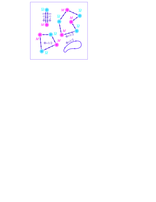
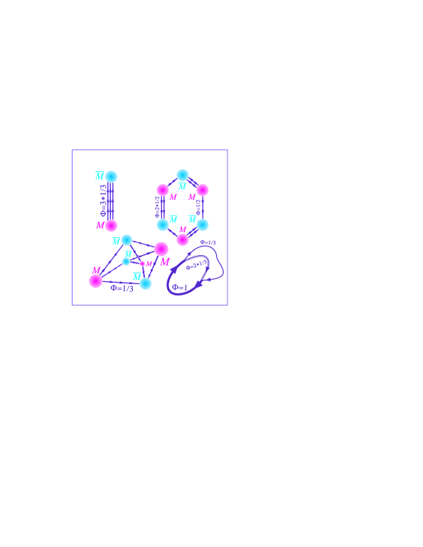
(a)	(b)

Figure 2: A schematic view of simplest vortex–monopole and pure vortex configurations in the cAHM₃ with (a) $Q=2$ and (b) $Q=3$ dynamical Higgs field.

In the case of $Q=3$ the monopoles and vortices may also form various structures like “benzene molecules”, non-planar nets etc., as seen in Figure 2(b). In the $Q=4$ case the monopole clusters must be similar to fullerene “cages” (carbon clusters).

II.3 Topological interactions

Let us consider now in more detail the contribution of the topological defects to the Wilson loop, $W_{q,Q}$, which defines the potential between two oppositely charged static external sources, $\langle W_{q,Q}\rangle\propto\exp\{-T\,V_{q,Q}(R)\}$. Here we have assumed that the Wilson loop has a rectangular shape, $T\times R$ with $T\gg R$. If no matter fields are coupled to the gauge field, $Q=0$, all non–perturbative contributions to the long-range potential would come from the monopole fields alone because the monopole fields are long-ranged in this case. In the presence of an electrically charged matter field, however, the magnetic fields are squeezed into vortices, which carry $\Phi=\frac{2\pi}{Q}$ units of magnetic flux. These vortices will provide the major contribution to the potential between external sources at large distances. The contribution of a general field configuration to the Wilson loop is $W^{{\cal C}}_{q,Q}=\exp\{i~{}q~{}\Phi_{\cal C}\}$. where $\Phi_{\cal C}$ is the Abelian flux going through the contour ${\cal C}$. Therefore each closed vortex trajectory $j_{0}$ contributes to the Wilson loop a factor

$$W^{{\cal C}}_{q,Q}=\exp\{2\pi i~{}\frac{q}{Q}~{}{I\!\!L}(j_{0},{\cal C})\}\,,$$ (4)

where ${I\!\!L}(j_{0},{\cal C})$ is the number of vortices piercing a surface spanned by the Wilson loop contour ${\cal C}$. The integer number ${I\!\!L}$ is an analogue of the linking number between vortex trajectories and the external particle trajectory discussed below.

The contribution of vortices to the Wilson loop quantum average in the form (4) may asymptotically lead to an area law provided the ratio $q/Q$ is not integer. An example of such a behavior is known from SU(2) gluodynamics where the so-called center vortices were shown to give a dominant contribution to the confinement of quarks ref:Greensite_Main . Thus, we expect that in the $Q>1$ cases the monopoles may form various types of clusters which range from simple wire-like structures to more complicated extended three-dimensional structures like nets etc.

The contribution of such vortices to the external particle potential depends on the ratio of the external charges, $q$, to the dynamical charges, $Q$. Eq. (4) states that if $\frac{q}{Q}\in{Z\!\!\!Z}$, then the contribution is trivial while in the case $\frac{q}{Q}\notin{Z\!\!\!Z}$ the vortices actually contribute to the Wilson loop average. In the latter case – as the analogy with SU(2) tells us – the Wilson loop may show the area law. Thus we conclude

$$\frac{q}{Q}\in{Z\!\!\!Z} \Leftarrow\Rightarrow \mbox{string breaking}\,,$$

$$\frac{q}{Q}\notin{Z\!\!\!Z} \Leftarrow\Rightarrow \mbox{no string breaking}\,.$$ (5)

It is quite instructive to reproduce these expectations by rewriting the partition function of the cAHM₃ in the London limit in terms of topological defects using the so-called Berezinsky-Kosterlitz-Thouless ref:KT ; ref:Berezinsky (BKT) transformation. For the sake of simplicity we use the Villain-type form of the action with couplings $\tilde{\beta}$ and $\tilde{\kappa}$. The cAHM₃ partition function in the Villain form has the form

$${\cal Z}=\int\limits^{\pi}_{-\pi}{\cal D}\theta\int\limits^{\pi}_{-\pi}{\cal D}\varphi\sum_{n(c_{2})\in{Z\!\!\!Z}}\sum_{l(c_{1})\in{Z\!\!\!Z}}\exp\Bigl{\{}-\tilde{\beta}{||\mathrm{d}\theta+2\pi n||}^{2}-\tilde{\kappa}{||\mathrm{d}\varphi-Q\,\theta+2\pi l||}^{2}\Bigr{\}}\,,$$ (6)

where $n$ and $l$ are integer-valued forms defined, respectively, on plaquettes, $c_{2}$, and links, $c_{1}$, of the lattice. Here and below we use the compact notations of differential forms on the lattice (for a review see, $e.g.$, Ref. Review:Monopole ). In brief, the plaquette angle $\theta_{P}$ on the plaquette $\{x,\mu\nu\}$ is written as ${(\mathrm{d}\theta)}_{x,\mu\nu}=\theta_{x,\mu}+\theta_{x+\hat{\mu},\nu}-\theta_{x+\hat{\nu},\mu}-\theta_{x,\nu}$. The gradient of the phase of the Higgs field belonging to the link $\{x,\mu\}$ is ${(\mathrm{d}\varphi)}_{x,\mu}=\varphi_{x+\hat{\mu}}-\varphi_{x}$. The Villain couplings are related to the original couplings as follows:

$$\tilde{\beta}(\beta)={\Bigl{[}2\log\frac{I_{0}(\beta)}{I_{1}(\beta)}\Bigr{]}}^{-1}\,,\quad\tilde{\kappa}(\kappa)={\Bigl{[}2\log\frac{I_{0}(\kappa)}{I_{1}(\kappa)}\Bigr{]}}^{-1}\,.$$ (7)

Let us apply the BKT transformation ref:KT ; ref:Berezinsky ; Review:Monopole first with respect to the gauge field in Eq. (6). The sum over the integer rank-two form $n$ in (6) can be rewritten in terms of a sum over an integer-valued one-form $p$ and an integer-valued three-form $m$,

$$\sum_{n(c_{2})\in{Z\!\!\!Z}}=\sum_{p(c_{1})\in{Z\!\!\!Z}}\sum_{m(c_{3})\in{Z\!\!\!Z}}\;,$$ (8)

using the decomposition

$$n=k[m]+\mathrm{d}p\,,\quad\mathrm{where}\quad\mathrm{d}k[m]=m\,.$$ (9)

Here $k[m]$ is an arbitrary integer two-form satisfying the second equation in (9). On the dual lattice ($i.e.$, on the lattice which is shifted by a half lattice spacing forward in all three directions) the form $\,\mbox{}^{\ast}m$ is an integer-valued scalar field (zero-form) constrained (due to the second equation in (9)) as follows:

$$\sum_{\,\mbox{}^{\ast}x}\,\mbox{}^{\ast}m_{\,\mbox{}^{\ast}x}=0\;,$$ (10)

what is equivalent to $\mathrm{d}m=0$ or $\delta\,\mbox{}^{\ast}m=0$ (with the co-derivative $\delta=\,\mbox{}^{\ast}\mathrm{d}\,\mbox{}^{\ast}$).

The integer-valued form $\,\mbox{}^{\ast}m$ represents, if non-vanishing, the presence of monopoles Review:Monopole on the sites of the dual lattice. For example, if exactly one monopole (antimonopole) resides in a particular cube $c_{3}$ of the original lattice, then the form $\,\mbox{}^{\ast}m$ is equal to $\pm 1$ at the corresponding site $\,\mbox{}^{\ast}x$. Equation (10) means that the total magnetic charge on the lattice is zero.

Using the Hodge-de-Rahm identity $1=\delta\Delta^{-1}\mathrm{d}+\mathrm{d}\Delta^{-1}\delta$ where $\Delta$ denotes the lattice Laplacian, the form $k[m]$ in Eq. (9) can be rewritten as $k[m]=\mathrm{d}\Delta^{-1}\delta k[m]+\delta\Delta^{-1}m$. Therefore the two-form $n$ can be written as $n=\delta\Delta^{-1}m+\mathrm{d}(\Delta^{-1}\delta k[m]+p)$ and we obtain the gauge invariant plaquette in the form

$$\mathrm{d}\theta+2\pi n=\mathrm{d}\theta^{\mathrm{n.c.}}+2\pi\delta\Delta^{-1}m\,,\quad\theta^{\mathrm{n.c.}}=\theta+2\pi\Delta^{-1}\delta k[m]+2\pi p\,,$$ (11)

where $\theta^{\mathrm{n.c.}}$ is a non-compact gauge field, i.e. $\theta^{\mathrm{n.c.}}_{l}\in(-\infty,+\infty)$. Moreover, the sum over the integer-valued variable $p$ and integration over the compact variable $\theta$ can be represented (again up to a volume-dependent factor) as an integration over the non-compact variable $\theta^{\mathrm{n.c.}}$.

Of course, the BKT transformation is nothing but a change of variables. After the first BKT transformation Eq. (6) reads as follows:

$${\cal Z}\propto\int\limits^{\infty}_{-\infty}{\cal D}\theta^{\mathrm{n.c.}}\int\limits^{\pi}_{-\pi}{\cal D}\varphi\sum_{\stackrel{{\scriptstyle\,\mbox{}^{\ast}m(\,\mbox{}^{\ast}c_{3})\in{Z\!\!\!Z}}}{{\delta\,\mbox{}^{\ast}m=0}}}\,\sum_{l^{\prime}(c_{1})\in{Z\!\!\!Z}}\exp\Bigl{\{}-\tilde{\beta}{||\mathrm{d}\theta^{\mathrm{n.c.}}||}^{2}-4\pi^{2}\,\tilde{\beta}(\,\mbox{}^{\ast}m,\Delta^{-1}\,\mbox{}^{\ast}m)$$

$$-\tilde{\kappa}{||\mathrm{d}\varphi-Q\,\theta^{\mathrm{n.c.}}+Q\cdot 2\pi\Delta^{-1}\delta k[m]+2\pi l^{\prime}||}^{2}\Bigr{\}}\,,$$ (12)

where we have used the basic relations of the differential lattice formalism: $\mathrm{d}^{2}=\delta^{2}=0$, $\Delta=\mathrm{d}\delta+\delta\mathrm{d}$, $\,\mbox{}^{\ast}\mathrm{d}\,\mbox{}^{\ast}=\delta$, and $*^{2}=1$. In addition, the original one-form $l$ is replaced through a shift by $l^{\prime}=l+Q\,p$ to make the link-dependent part of the action (proportional to $\tilde{\kappa}$) independent of $p$. The global condition (10) is implicitly understood in Eq. (12) and subsequent equations.

Next, we apply the BKT transformation a second time, with respect to the compact phase of the Higgs field. We proceed similarly to the case of the compact gauge field, representing the sum over the one-form $l^{\prime}$ as sums over some two-form $j$ and a zero-form $r$. The forms $j$ and $r$ are related to $l^{\prime}$ as follows:

$$l^{\prime}=s[j]+\mathrm{d}r\,,\quad\mathrm{where}\quad\mathrm{d}s[j]=j\,.$$ (13)

Again using the Hodge-de-Rahm identity we introduce the non-compact scalar field $\varphi^{\mathrm{n.c.}}$:

$$\mathrm{d}\varphi+2\pi l^{\prime}=\mathrm{d}\varphi^{\mathrm{n.c.}}+2\pi\delta\Delta^{-1}j\,,\quad\varphi^{\mathrm{n.c.}}=\varphi+2\pi\Delta^{-1}\delta s[j]+2\pi r\,.$$ (14)

The partition function (12) is now written as follows:

$${\cal Z}\propto\int\limits^{\infty}_{-\infty}{\cal D}\theta^{\mathrm{n.c.}}\int\limits^{\infty}_{-\infty}{\cal D}\varphi^{\mathrm{n.c.}}\sum_{\stackrel{{\scriptstyle\,\mbox{}^{\ast}m(\,\mbox{}^{\ast}c_{3})\in{Z\!\!\!Z}}}{{\delta\,\mbox{}^{\ast}m=0}}}\,\sum_{\stackrel{{\scriptstyle\,\mbox{}^{\ast}j(\,\mbox{}^{\ast}c_{2})\in{Z\!\!\!Z}}}{{\delta\,\mbox{}^{\ast}j=0}}}\exp\Bigl{\{}-\tilde{\beta}{||\mathrm{d}\theta^{\mathrm{n.c.}}||}^{2}-4\pi^{2}\,\tilde{\beta}(\,\mbox{}^{\ast}m,\Delta^{-1}\,\mbox{}^{\ast}m)$$

$$-\tilde{\kappa}{||\mathrm{d}\varphi^{\mathrm{n.c.}}-Q\,\theta^{\mathrm{n.c.}}+2\pi\Delta^{-1}\delta(j+Q\,k[m])||}^{2}\Bigr{\}}\,.$$ (15)

The integer-valued one-form

$$\,\mbox{}^{\ast}j_{m}=Q\,\mbox{}^{\ast}k[m]+\,\mbox{}^{\ast}j$$ (16)

represents, if non-vanishing, the vortex line defined on a dual link, similarly to the monopole zero-form $\,\mbox{}^{\ast}m$. The constraint

$$\delta\,\mbox{}^{\ast}j_{m}=Q\,\mbox{}^{\ast}m$$ (17)

(whereas $\delta\,\mbox{}^{\ast}j=0$) indicates conservation of magnetic flux: vortices carry a fraction ${1}/{Q}$ of the total magnetic flux emanating from a monopole or absorbing by an anti-monopole.

It is self-evident that the definitions, introduced in passing, of monopoles $\,\mbox{}^{\ast}m$ and vortices $\,\mbox{}^{\ast}j_{m}$ are identical to those obtained directly from the gauge invariant plaquette $P=\mathrm{d}\theta+2\pi n$

$$m=\frac{\mathrm{d}P}{2\pi}=\mathrm{d}n\,,\quad\mathrm{d}m=0$$ (18)

and the link $L=\mathrm{d}\varphi-Q\,\theta+2\pi l$

$$j_{m}=\frac{\mathrm{d}L+Q\,P}{2\pi}=\mathrm{d}l+Q\,n\,,\quad\mathrm{d}j_{m}=Q\,m\,.$$ (19)

Performing the Gaussian integration over the non-compact fields  in Eq. (15) we rewrite the partition function in terms of monopoles and vortices:

$${\cal Z}=\sum_{\stackrel{{\scriptstyle\,\mbox{}^{\ast}m(\,\mbox{}^{\ast}c_{3})\in{Z\!\!\!Z}}}{{\delta\,\mbox{}^{\ast}m=0}}}\,\sum_{\stackrel{{\scriptstyle\,\mbox{}^{\ast}j_{m}(\,\mbox{}^{\ast}c_{2})\in{Z\!\!\!Z}}}{{\delta\,\mbox{}^{\ast}j_{m}=Q\,\mbox{}^{\ast}m}}}\exp\Bigl{\{}-S_{d}(\,\mbox{}^{\ast}m,\,\mbox{}^{\ast}j_{m})\Bigr{\}}\,.$$ (20)

The action of the topological defects is

$$S_{d}(\,\mbox{}^{\ast}m,\,\mbox{}^{\ast}j_{m})=4\pi^{2}\tilde{\beta}(\,\mbox{}^{\ast}m,\frac{1}{\Delta+M^{2}}\,\mbox{}^{\ast}m)+4\pi^{2}\tilde{\kappa}(\,\mbox{}^{\ast}j_{m},\frac{1}{\Delta+M^{2}}\,\mbox{}^{\ast}j_{m})\,,$$ (21)

where $M=Q{(\tilde{\kappa}/\tilde{\beta})}^{1/2}$ is the tree-level mass of the gauge boson.

Let us now consider the contribution of the vortices and monopoles to the potential $V_{q,Q}(R)$ between a pair of external particles with charges $\pm q$, separated by a distance $R$. The potential is given by the quantum average of the Wilson loop defined as

$$\langle W_{q}(J)\rangle_{Q} = \frac{1}{{\cal Z}}\int\limits_{-\pi}^{\pi}{\cal D}\theta\int\limits_{-\pi}^{\pi}{\cal D}\varphi\sum_{n(c_{2})\in{Z\!\!\!Z}}\,\sum_{l(c_{1})\in{Z\!\!\!Z}}\times$$ (22)

$$\exp\Bigl{\{}-\tilde{\beta}||\mathrm{d}\theta+2\pi n||^{2}-\tilde{\kappa}||\mathrm{d}\varphi-Q\theta+2\pi l||^{2}+iq(J,\theta)\Bigr{\}}\,.$$

The external current satisfies $\delta J$=0.

Following the transformations which led us from Eq. (6) to Eq. (20), the v.e.v. of the Wilson loop can be rewritten as

$$\langle W_{q}\rangle_{Q}=\langle W_{q}\rangle_{\mathrm{ph}}\,\langle W_{q}\rangle_{d}\,.$$ (23)

Here

$$\langle W_{q}\rangle_{\mathrm{ph}}\propto\exp\Bigl{\{}-\frac{q^{2}}{4\tilde{\beta}}\,(J,\frac{1}{\Delta+M^{2}}J)\Bigr{\}}$$ (24)

is the perturbative self-interaction contribution of the external loop given by exchange of a massive photon, while the non-perturbative factor is due to the topological defects:

$$\langle W_{q}\rangle_{d}=\frac{1}{{\cal Z}_{d}}\sum_{\stackrel{{\scriptstyle\,\mbox{}^{\ast}m(\,\mbox{}^{\ast}c_{3})\in{Z\!\!\!Z}}}{{\delta\,\mbox{}^{\ast}m=0}}}\,\sum_{\stackrel{{\scriptstyle\,\mbox{}^{\ast}j_{m}(\,\mbox{}^{\ast}c_{2})\in{Z\!\!\!Z}}}{{\delta\,\mbox{}^{\ast}j_{m}=Q\,\mbox{}^{\ast}m}}}\exp\Bigl{\{}-S_{d}(\,\mbox{}^{\ast}m,\,\mbox{}^{\ast}j_{m})-S_{\mathrm{int}}(\,\mbox{}^{\ast}m,\,\mbox{}^{\ast}j_{m};J)\Bigr{\}}$$ (25)

with

$$S_{\mathrm{int}}=-2\pi i\frac{q}{Q}(\delta j_{m},\frac{1}{\Delta+M^{2}}J)+2\pi i\frac{q}{Q}{I\!\!L}(\,\mbox{}^{\ast}j_{0},J)\,.$$ (26)

The first term in $S_{\mathrm{int}}$ consists of a Yukawa-type interaction between the vortices and the external charged particle. Since the vortices and the monopoles are related to each other by the constraint (17), the first term in $S_{\mathrm{int}}$ also represents an indirect interaction between the monopoles and the external charged particle.

The second term is of topological nature. It is given by the linking number

$${I\!\!L}(\,\mbox{}^{\ast}j_{0},J)=(\delta j_{0},\Delta^{-1}J)\in{Z\!\!\!Z}$$ (27)

between the external particle trajectory $J$ and the one-form $\,\mbox{}^{\ast}j_{0}$. The form $\,\mbox{}^{\ast}j_{0}$ is derived from the vortex ensemble $\,\mbox{}^{\ast}j_{m}$ by subtracting $Q\,\mbox{}^{\ast}k[m]$, cf. (16), such that $\delta\,\mbox{}^{\ast}j_{0}=0$. In contrast to $\,\mbox{}^{\ast}j_{m}$, the modified vortex ensemble $\,\mbox{}^{\ast}j_{0}$ consists of oriented and closed loops. The linking number between $\,\mbox{}^{\ast}j_{0}$ and $J$ corresponds to the Aharonov-Bohm (AB) effect ref:MIP_Zubkov .

In the cQED-like limit, $M\to 0$, the interaction term (26) reduces to the usual cQED-like interaction between monopoles:

$$\lim\limits_{M\to 0}S_{\mathrm{int}} = -2\pi i\frac{q}{Q}(\delta j_{m},\Delta^{-1}J)+2\pi i\frac{q}{Q}{I\!\!L}(\,\mbox{}^{\ast}j_{0},J)$$ (28)

$$= 2\pi i\frac{q}{Q}(\delta(j_{0}-j_{m}),\Delta^{-1}J)=-2\pi i(k[m],\Delta^{-1}J)\,,$$

where we have used Eq. (27) and Eq. (16). The interaction (28) does not depend on the shape of the Dirac line, $\,\mbox{}^{\ast}k[m]$, and does depend on the monopole magnetic charges and monopole locations, $\,\mbox{}^{\ast}m\equiv\delta\,\mbox{}^{\ast}k[m]$.

Note that the separation of a general vortex ensemble, $\,\mbox{}^{\ast}j_{m}=\,\mbox{}^{\ast}j_{0}+\,\mbox{}^{\ast}j_{m}^{\prime}$, into closed vortices, $\delta\,\mbox{}^{\ast}j_{0}=0$, and open ones, $\delta\,\mbox{}^{\ast}j_{m}^{\prime}=\,\mbox{}^{\ast}m$, is ambiguous. In the sum (25) the ambiguity disappears since all ambiguous separations enter Eq. (25) with the same weight.

The contribution of vortices to the inter-particle potential $V_{q,Q}(R)$ is twofold. First, the closed vortices $\,\mbox{}^{\ast}j_{0}$ interact with the electrically charged particles via the AB effect if the ratio $q/Q$ is not integer. Secondly, the vortices influence the monopole dynamics via the constraint (17), contributing in this way to the potential indirectly, via the monopoles and their interaction with the test particles.

Actually, orientable vortices with closed magnetic flux lines cannot lead to confinement of electric charges ref:GubarevAHM . In that paper numerical studies for the non-compact version of the AHM₃ have shown that confinement is not realized. This is a model in which orientable vortices are present (and consequently, an AB effect might be at work) whereas magnetic monopoles are absent. On the other hand, a long-range interaction between vortices and the electric Wilson loop may be provided only by the AB effect in a form visible in Eq. (25). In the model presently under consideration the linking of the non-orientable vortices with the external electric current is formally expressed by (27) in terms of the redefined closed and orientable loops $\,\mbox{}^{\ast}j_{0}$. Making this point, we are implicitly leaning upon that we are working in a model with a mass gap in which any interactions – except for topological ones like the one mediated by the linking number – must be suppressed.

In four dimensional QCD the so-called center vortices are known to lead to the area law of the Wilson loop via the AB interaction ref:Greensite_Main . They are providing a dominant contribution to the confinement of quarks if they are localized by means the so-called Maximal Center projection. There is no contradiction between the roles of the AB effect in QCD and the non-compact AHM since in the QCD case the center vortices are non-orientable worldsheets whereas in the case of the 3D non-cAHM they are orientable lines. Moreover, considered in an Abelian sense, the non-orientable center vortices can be represented as piecewise orientable vortices with monopole trajectories separating segments with different flux orientations from each other. The required non-orientability implies the existence of monopoles living on the vortex sheets.

We will see that all percolating loops in the case of the model studied here (which are responsible for confinement) really form an alternating monopole-antimonopole chain which makes them physically non-orientable. Thus, we expect that in cAHM₃ the vortices play a role to accomplish both confinement and string breaking phenomena, for the respective sources, by restructuring the monopoles configurations.

III Phase structure in the London limit and the percolation properties of monopole chains

III.1 The finite-temperature case

In this subsection we report on our numerical study of the confining properties as seen by static external particles with different electric charges $q$ in the case of the cAHM₃ with doubly–charged matter. In the confining phase of this model only external particles with charge $q=1$ must be asymptotically confined while particles with charge $q=2$ should experience the flattening of the potential at large distances.

To observe this effect we have simulated the model (3) first on lattices $32^{2}\times 8$. The choice of the asymmetric lattice (finite $T$) was not a matter of principle but simply dictated by the fact that in the case of symmetric ($L^{3}$) lattices the potential can be measured only using Wilson loops which are notoriously unsuitable for an observation of the string breaking effect. We have performed simulations at fixed gauge coupling constant, $\beta=1.2$, the choice of which was motivated by visualization reasons. Indeed, in order to clearly see the monopole structures, the density of the monopoles must be neither too high nor too low. According to Eq. (21) a singly–charged (anti)monopole enters the partition function with the action $S^{(1)}_{m}=4\pi^{2}\tilde{\beta}\,\Delta^{-1}(0)$ (with $\Delta^{-1}(0)\approx 0.25$ in the thermodynamic limit). Thus an increase (decrease) of the gauge coupling $\beta$ constant suppresses (enhances) the number of monopoles. The chosen value of $\beta$ is ideal from the point of view of our purposes. We have used about $10^{5}$ configurations for each value of the hopping parameter $\kappa$. Some results on the finite–temperature case (partially included in this subsection) were previously reported in Ref. ref:U1Q2PLB .

To probe the phase structure of the model we first study the vacuum expectation values (v.e.v.’s) of the $q=1$ and $q=2$ Polyakov loops,

$$L_{q}(\vec{x})=\exp\{iq\sum_{t=1}^{L_{t}}\theta_{4}(\vec{x},t)\}\,.$$ (29)

Their expectation values are shown in Figure 3(a)

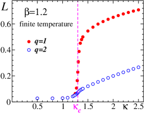
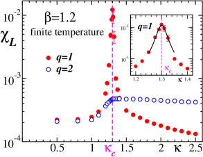
(a)	(b)

Figure 3: The $q=1,2$ Polyakov loops (a) and their susceptibilities vs. $\kappa$ at $\beta=1.2$ on a $32^{2}\times 8$ lattice. The insert in Figure (b) shows the behavior of the $q=1$ susceptibility in the vicinity of the phase transition with the fit according to Eq. (30).

as a function of the hopping parameter $\kappa$. At small (large) $\kappa$ the $v.e.v.$’s of both loops are low (high) corresponding to the confinement (Higgs) phase. One can clearly see that the (outside the Higgs phase) confined $q=1$ external charges more sensitively react to the onset of the Higgs phase compared to the $q=2$ charges. This is a typical signature of the $q=2$ string breaking. The abundantly available $Q=2$ particles screen $q=2$ external charges which leads to the low sensitivity of the $q=2$ loops to the phase transition.

In Figure 3(b) we show the Polyakov loop susceptibilities vs. $\kappa$. The $q=2$ susceptibility does not indicate any significant change at the transition point while the $q=1$ susceptibility shows a sharp peak signalling the presence of a phase transition. We have fitted the $q=1$ susceptibility in the vicinity of the maximum by the function Chernodub:2002ym :

$$\chi^{\mathrm{fit}}(\kappa)=\frac{C_{1}}{{(C_{2}+{(\kappa-\kappa_{c})}^{2})}^{\gamma_{\chi}}}\,,$$ (30)

with $C_{1,2}$, $\gamma_{\chi}$ and $\kappa_{c}$ being the fit parameters. From the fit (shown in the insert of Figure 3(b) as a solid line) we obtain that the transition happens at

$$\kappa_{c}\equiv\kappa^{q=1}_{c}=1.300(1)\,.$$ (31)

To fit the susceptibility in the vicinity of the critical value we have chosen the region such that $\chi^{2}/d.o.f.\sim 1$. This choice applies to all fits of susceptibilities performed in this paper.

The static potentials between $q$–charged external particles can be expressed via the Polyakov loop correlators, $V_{q,Q}(R)=-L^{-1}_{t}\,\log\langle L_{q}({\vec{0}})L^{*}_{q}({\vec{R}})\rangle$. As it was shown in Ref. ref:U1Q2PLB , in the confinement phase the potential for the $q=1$ external charges is linearly rising at large distances while $q=2$ potential shows a rapid flattening corresponding to dynamical particles popping up from the vacuum to cause string breaking. In the Higgs phase all potentials suffer flattening due to deconfining nature of this phase. The corresponding potentials are shown in Figure 4.

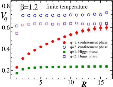
Figure 4: The $q=1,2$ potentials in the confinement ($\kappa=1.275$) and the Higgs ($\kappa=1.325$) phases at $\beta=1.2$ (from Ref. ref:U1Q2PLB ).

This result completely agrees with the general form of the phase diagram shown in Figure 1.

As we have mentioned above, the cAHM contains two types of topological objects – monopoles and vortices. The simplest characteristic of a topological defect is its density. The monopole and the vortex densities are (the volume is $V=L^{2}L_{t}$ for finite temperature and $V=L^{3}$ at $T=0$)

$$\rho_{\mathrm{mon}}=\frac{1}{V}\sum_{\,\mbox{}^{\ast}c_{3}}|\,\mbox{}^{\ast}m|\,,\qquad\rho_{\mathrm{vort}}=\frac{1}{3V}\sum_{\,\mbox{}^{\ast}c_{2}}|\,\mbox{}^{\ast}j_{m}|\,,$$ (32)

respectively. The monopole charge is defined in the standard way (see also (18)),

$$m=\frac{1}{2\pi}\mathrm{d}{[\mathrm{d}\theta]}_{2\pi}\,,$$ (33)

where ${[\cdots]}_{2\pi}/(2\pi)$ denotes the integer part modulo $2\pi$. Following Ref. ANO_definition , the vortex current is defined as (cf. (19))

$$j=\frac{1}{2\pi}(\mathrm{d}{[\mathrm{d}\varphi+\,\theta]}_{2\pi}-Q{[\mathrm{d}\theta]}_{2\pi})\,.$$ (34)

According to Figure 5(a)

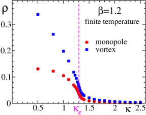
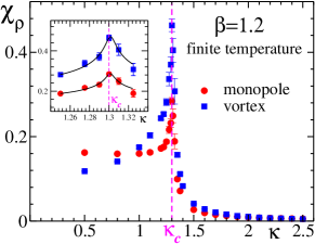
(a)	(b)

Figure 5: (a) The monopole and vortex densities (from Ref.ref:U1Q2PLB ) and (b) their susceptibilities, $vs.$ $\kappa$ at $\beta=1.2$ on $32^{2}\times 8$ lattice. The insert in Figure (b) shows the behavior of the susceptibilities in the vicinity of the phase transition. The solid lines show the fits by Eq. (30).

the densities (exposed in lattice units) of both monopoles and vortices are gradually decreasing functions of the coupling $\kappa$ what is partly a finite temperature effect. In the confinement (Higgs) phase the density of both vortices and monopoles is high (low), in agreement with the expectation that the confining properties of the cAHM₃ are due to topological defects. Both susceptibilities are peaked at the phase transition point. The fits by Eq. (30) of the monopole and vortex susceptibilities give the following transition values of the hopping parameter, respectively:

$$\kappa^{\mathrm{mon}}_{c}=1.301(3)\,,\qquad\kappa^{\mathrm{vort}}_{c}=1.302(2)\,.$$ (35)

These values are consistent with each other as well as with the critical value obtained with the help of the $q=1$ Polyakov loop susceptibility discussed above.

Obviously, in the confining phase the monopoles cannot form a monopole or dipole plasma because in these cases both external charges $q=1,2$ would be simultaneously confined or deconfined. Thus the only possible kind of monopole configurations – which can explain both the linearly rising potential for the $q=1$ electric charges and the string breaking for the $q=2$ charges – is a monopole chain schematically plotted in Figure 2(a). In a monopole chain the monopoles and antimonopoles are mutually alternating. Thus the magnetic flux coming from a monopole inside the chain is separated into two parts, squeezed into the vortices and, as a consequence, forming a non-orientable closed magnetic flux. Each piece of such a vortex carries (in average) a half flux, $\Phi=\frac{2\pi}{Q}\equiv\pi$. If such a flux pierces the $q$-charged Wilson loop it provides a (multiplicative) contribution to the loop close to ${(-1)}^{q}$. This leads to a disorder for odd charged external particles (eventually leading to a linearly rising potential) whereas particles with even charge are not confined. The described picture is very similar to what is observed ref:Greensite_correlations in QCD for the correlations between the Abelian monopoles and the center vortices.

In Figures 6(a-d)

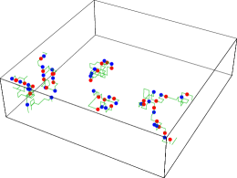
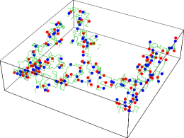
(a)	(b)
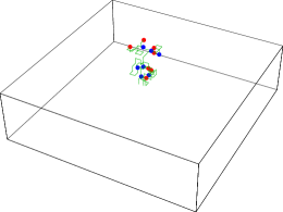
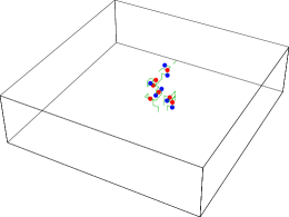
(c)	(d)

Figure 6: Examples of the monopole configurations in the confinement phase at $\kappa=1.275$ (upper row) and in the deconfinement (Higgs) phase at $\kappa=1.325$ (lower row). The (anti-)monopoles are shown by the dots while the vortices are shown by the solid lines.

we show typical monopole configurations observed in our numerical simulations. In the confining phase the monopoles form chains which either wrap around the temperature direction (Figure 6(a)) or fill all the lattice volume (Figure 6(b)). In the last case the monopole chains are said to be percolating. In the Higgs phase the monopole chains wrap only around the temperature direction (Figure 6(c,d)). In the next subsection we investigate the percolation properties of the monopole chains in the zero–temperature model. We want to demonstrate that the mechanism causing the confining/deconfining effects is the same as for the finite temperature lattice dealt with in this subsection.

III.2 The zero-temperature case at fixed gauge coupling $\beta=2.0$

We report now the study of the doubly–charged cAHM at zero-temperature, on the lattice $16^{3}$. From $2\cdot 10^{3}$ to $8\cdot 10^{4}$ measurements for every $\beta,\kappa$ pair have been collected. First we map out the phase structure along a vertical line at $\beta=2.0$ in the phase diagram Fig. 1, varying the hopping parameter $\kappa$. We mainly concentrate on the quantitative analysis of the monopole chains and their components, vortices and monopoles.

Similarly to the finite–temperature case, for orientational purposes, we measure the expectation values of the Polyakov loops which also in the zero–temperature model is defined as a Wilson line closed via the boundary conditions. The expectation values of the $q=1,2$ Polyakov loops are shown in Figure 7(a).

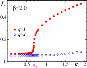
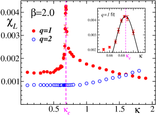
(a)	(b)

Figure 7: (a) The expectation values of the Polyakov loop for $q=1$ and $q=2$ and (b) their susceptibilities vs. $\kappa$ for a lattice $16^{3}$. The insert in Figure (b) shows the behavior of the $q=1$ susceptibility in the vicinity of the phase transition and the fit according to Eq. (30).

As in the finite $T$ case the v.e.v. of the $q=1$ Polyakov loop is noticeably larger in the Higgs phase (larger $\kappa$’s) and almost constant in the confinement phase (smaller $\kappa$’s). The $q=2$ Polyakov loop is almost constant crossing the transition. Consequently, the $q=1$ susceptibility of the Polyakov loop is peaked at the transition point for moderate lattice volume while the susceptibility of the $q=2$ line is insensitive to the transition. The fit of the $q=1$ susceptibility by Eq. (30) is shown in the insert of Figure 7(b) as a solid line. The corresponding critical value of the hopping parameter is

$$\kappa_{c}\equiv\kappa^{q=1}_{c}=0.687(1)\,.$$ (36)

To clarify the role of the topological defects we plot the density of defects in Figure 8(a).

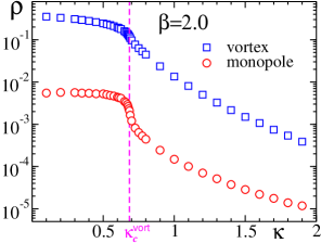
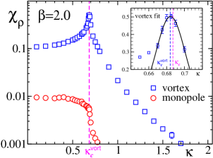
(a)	(b)

Figure 8: (a) The densities of the topological defects and (b) their susceptibilities vs. $\kappa$. The insert in Figure (b) shows the behavior of the vortex susceptibility in the vicinity of the phase transition. The solid line shows the fit by Eq. (30).

One can clearly see that in this region of the phase diagram the density of monopoles is much smaller than the density of vortices. This is not unexpected since at $\beta=2.0$ the action of an isolated monopole is $S^{(1)}_{m}=4\pi^{2}\tilde{\beta}\,\Delta^{-1}(0)\approx 20$, therefore the monopoles must be suppressed drastically. One may therefore conjecture that at $\beta=2.0$ the leading role at the transition should be played by vortices and not by the monopoles, in other words, the dynamics of the monopoles is driven by the vortex networks.

In Figure 8(b) we show the susceptibilities of the monopole and vortex densities. The vortices are sensitive to the phase transition while the susceptibility of the monopole density does not show any noticeable peak at the critical value of the hopping parameter. The fit of the susceptibility of the vortex density by function (30) gives the pseudo-critical value of the hopping parameter

$$\kappa^{\mathrm{vort}}_{c}=0.684(3)\,,$$ (37)

consistent with the value obtained from the susceptibility of the Polyakov loop.

To characterize quantitatively the behavior of the clusters we plot in Figure 9(a)

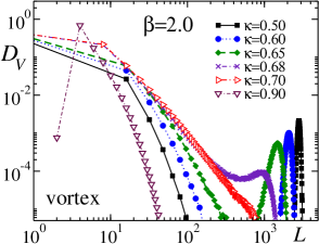
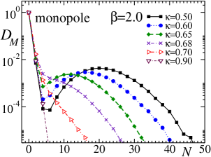
(a)	(b)

Figure 9: Histograms of the (a) vortex and (b) monopole distributions.

the distribution $D_{V}$ of the lengths $L$ of the vortices inside the (mutually disconnected) clusters. The distributions for various $\kappa$ are normalized to unity. To see the difference between the phases, we plot the distributions for $\kappa$ values in the vicinity of the phase transition. One can see that in the confinement phase the vacuum is populated by two different types of clusters since the distributions have two peaks. The vortex lengths in the first type of clusters is typically short. The vortices of this type are called ultraviolet vortices. The term “ultraviolet” is borrowed from $4D$ QCD which also possesses Abelian monopole trajectories (defined in an Abelian projection) which fall into similar classes of loops. In QCD the ultraviolet monopoles can be described by a formula $D_{M}^{UV}\sim L^{-\lambda}$ where $\lambda$ is a positive number which does not depend on the lattice volume ref:clusters . This experience leads us to conjecture a similar behavior in the $3D$ cAHM as well, except that the loops are now formed by vortices.

The other population of vortices consists of the so called “infrared” vortices which form the second peak in the distribution $D_{V}$. The average number of the length $L$ of the vortices in this peak is proportional to the number of links on the lattice, $3V$, multiplied by an “infrared density” $\rho^{V}_{IR}$ which may be also referred to as the “vortex condensate”. The vortices from this condensate occupy uniformly all the volume of the system and their typical length is equal to $\rho^{V}_{IR}\,3V$. The fluctuations of the length of the infrared clusters are expected to be random. Therefore, they may be described by a Gaussian ansatz (here we refer to Ref. ref:gaussian_QCD where a similar observation was made for monopole trajectories). It is clear that the vortex condensate exists only in the confinement phase (signalled by the infrared peak of the histogram) while it is absent in the Higgs (deconfinement) phase

A similar behavior is also observed for the distributions $D_{M}$ with respect to the monopole number $N$ inside the mutually disconnected vortex clusters. Monopoles are pointlike and connected by vortices. These distributions are plotted in Figure 9(b). One can also see the two-peak structure in the confinement phase (the infrared and the ultraviolet monopoles corresponding to long and short vortex clusters) and the disappearance of the infrared peak in the Higgs (deconfinement) phase.

From Figures 9(a,b) we conclude that in the confinement phase a vortex condensate is formed. The percolating vortices are carrying the monopoles which are responsible for the confining properties of the vacuum.

In order to characterize the cluster distributions of vortices and monopoles $D_{V,M}$ we fitted the distribution functions by

$$D^{\mathrm{fit}}_{V}(L)=C_{1,V}\,L^{-\lambda_{V}}+C_{2,V}\,\exp\Bigl{\{}-\alpha_{V}(L-\rho^{V}_{IR}\cdot 3V)^{2}\Bigr{\}}$$ (38)

and by an analogous form for the monopole distributions

$$D^{\mathrm{fit}}_{M}(N)=C_{1,M}\,N^{-\lambda_{M}}+C_{2,M}\,\exp\Bigl{\{}-\alpha_{M}(N-\rho^{M}_{IR}\cdot V)^{2}\Bigr{\}}$$ (39)

to determine the condensates $\rho^{V,M}_{IR}$. Equations (38) and (39) describe the distribution of the topological defects as the sum of an ultraviolet component (first, inverse power term) and an infrared component (second, Gaussian term).

As we have seen, the second (infrared) peaks in the monopole number and vortex length distributions are absent in the deconfinement phase. Therefore we fit the distributions by Eqs. (38) and (39) only in the confinement phase. The fits of the vortex length distributions are shown in Figure 10(a).

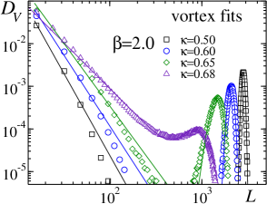
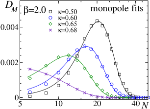
(a)	(b)

Figure 10: Fits of (a) the monopole and (b) the vortex histograms by Eqs. (38) and (39).

One can see that the fitting function describes well the data both in the low-$L$ and high-$L$ regions. To fit the monopole distributions we have set $C_{1,M}=0$ since there is not enough data to fix the ultraviolet part of the distribution. We have performed the fit for $N\geqslant 6$ as it is shown in Figure 10(b).

The densities of vortices and monopoles in infrared clusters are shown in Figure 11 as a function of $\kappa$ in the confining phase.

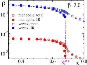
Figure 11: The densities of topological defects in infrared clusters as given by fits (38) and (39). The fits by Eq. (40) are shown by dashed lines.

One observes that the density of the infrared part of both types of topological defects drops down when the phase transition point is approached, in agreement with our expectations. Deeper in the confining phase the infrared densities are practically saturating the total densities.

We have fitted the infrared densities of both types of topological defects by functions of the form

$$\rho^{V,M}_{IR}(\kappa)=B_{V,M}\cdot(\kappa_{c}^{V,M}-\kappa)^{\gamma^{V,M}}\,,\qquad\kappa<\kappa_{c}\,,$$ (40)

assuming a “critical behavior” near the phase transition. Both fits are shown in Figure (11) as dashed lines. The transition points are:

$$\kappa^{M}_{c}=0.680(3)\,,\qquad\kappa^{V}_{c}=0.684(1)$$ (41)

from the infrared monopole and vortex densities, respectively. They are in agreement with each other as well as with the values determined by from the susceptibilities of the Polyakov loops and the vortex density. The “critical exponents” are different: $\gamma^{M}=0.28(2)$ and $\gamma^{V}=0.37(1)$.

Yet another interesting aspect of the cluster structure is the cluster multiplicity distribution $D(N_{cl})$ which represents the total number of vortex clusters per configuration (irrespective of the cluster size). We show $D(N_{cl})$ for various values of hopping parameter $\kappa$ in Figure 12. The distribution of the cluster number can be well described by a Gaussian function,

$$D(N_{cl})=A\exp\Bigl{\{}-\frac{(N_{cl}-\bar{N}_{cl})^{2}}{2\Lambda}\Bigr{\}}\,.$$ (42)

The fits are shown in Figure 12 as solid lines.

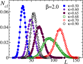
Figure 12: The multiplicity distributions of vortex clusters and the corresponding fits by the Gaussian distribution (42) for various $\kappa$ values.

The fitted average cluster multiplicity $\bar{N}_{cl}$ and the width of the distribution $\Lambda$ are presented in Figure 13 as functions of $\kappa$.

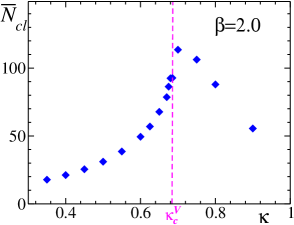
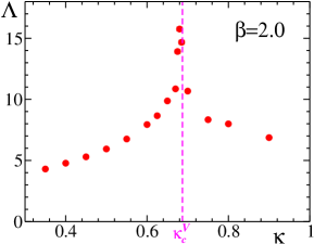
(a)	(b)

Figure 13: (a) The average number $\bar{N}_{cl}$ of clusters and (b) the width $\Lambda$ of the multiplicity distribution as functions of $\kappa$.

Both parameters are peaked near the phase transition indicating that at the critical value of the hopping parameter the few large infrared clusters – existing in the confinement phase – decompose into many smaller clusters as the system goes over into the deconfinement phase. According to Figure 8(a) the monopole and vortex densities drop slightly with increasing $\kappa$ at $\kappa_{c}$. Therefore, the increase of the cluster number is associated predominantly with a cluster–restructuring process and not with a cluster creation phenomenon. Moreover, the increase of the width $\Lambda$ indicates the existence of large fluctuations in the vortex system at $\kappa\approx\kappa_{c}$.

III.3 The zero-temperature case at fixed hopping parameter $\kappa=1.0$

In this subsection we map out the phase structure along an horizontal line through the phase diagram of Fig. 1. At $\kappa$ as large as $\kappa=1.0$ the confinement phase is realized only for relatively small $\beta$. In Fig. 14

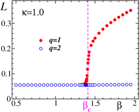
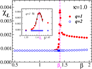
(a)	(b)

Figure 14: (a) The expectation values of the Polyakov loop and (b) their susceptibilities vs. $\kappa$. The insert in Figure (b) shows the behavior of the $q=1$ susceptibility in the vicinity of the phase transition together with its fit.

we show the v.e.v.’s of the $q=1$ and $q=2$ Polyakov loops vs. $\beta$. Only the susceptibility of the $q=1$ Polyakov loop shows a peak which leads to an estimate

$$\beta_{c}\equiv\beta_{c}^{q=1}=1.410(2)$$ (43)

using a fitting function $\chi^{\rm fit}(\beta)$ analogously to (30). The position of the phase transition defined from the fit of the $q=1$ Polyakov loop is shown by a vertical dashed line.

In the confining phase we have now a density of monopoles comparable in magnitude to the density of vortices. In Fig. 15

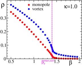
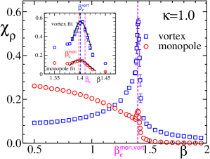
(a)	(b)

Figure 15: (a) The densities of the topological defects and (b) their susceptibilities vs. $\beta$. The insert in Figure (b) shows the behavior of the monopole and vortex susceptibilities in the vicinity of the phase transition with their fits and critical $\beta$’s.

we show both densities and the respective susceptibilities. Values as $\beta=2.0$ which have led to a vortex–driven transition described in the previous subsection are now belonging to the deconfinement phase. The peak of the susceptibility of the vortex density is still more pronounced at the transition, but now the susceptibility of the monopole density also shows a little peak.

The positions of the peaks for the monopole and vortex susceptibilities are slightly shifted compared to the peak of the $q=1$ Polyakov loop susceptibility, Fig. 14. The fits of the monopole and vortex susceptibilities in the vicinity of the phase transition give the following values for $\beta_{c}$ corresponding to the transition, respectively:

$$\beta_{c}^{\mathrm{mon}}=1.398(1)\,,\qquad\beta_{c}^{\mathrm{vort}}=1.401(1)\,.$$ (44)

One can see that the couplings $\beta_{c}$ obtained with the help of the monopole and vortex susceptibilities are very similar to each other.

Histograms of the vortex length an monopole number distribution for the individual vortex clusters are shown in Fig. 16

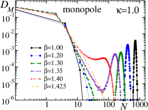
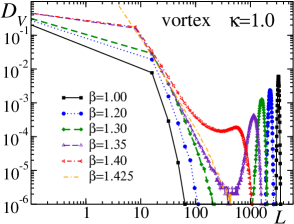
(a)	(b)

Figure 16: Histograms of the (a) monopole and (b) vortex distributions.

for various $\beta$ values near $\beta_{c}$. Fits corresponding to the two-component forms (38) and (39) are presented in Fig. 17.

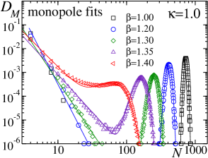
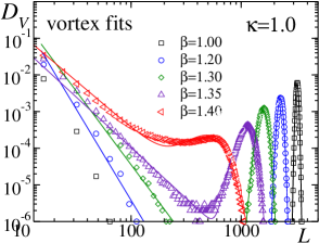
(a)	(b)

Figure 17: Fits of (a) the monopole and (b) the vortex histograms by Eqs. (38) and (39).

The fitted values of the infrared monopole and vortex densities are shown in Fig. 18

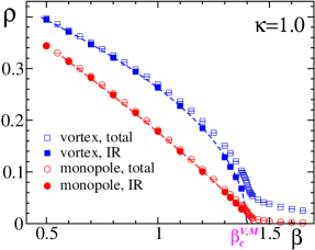
Figure 18: The densities of the topological defects in infrared clusters as given by fits (38) and (39). The fit curves using $\rho^{M,V}_{IR}(\beta)$ similar to Eq. (40) are shown by dashed lines.

together with the total densities as functions of $\beta$. Again deeper in the confining phase the infrared densities practically saturate the total densities. The respective $\beta_{c}$–values marking the transition from the infrared clusters are found fitting the $\beta$-dependence with an ansatz $\rho^{M,V}_{IR}(\beta)$ similar to Eq. (40). The fit curves are shown in the Figure as well. The corresponding critical values extracted from the infrared monopole and the vortex densities are:

$$\beta^{M}_{c} = 1.424(3)\,,\qquad\beta^{V}_{c}=1.399(2)\,.$$ (45)

The “critical exponents” are rather different again: $\gamma^{M}=0.86(1)$ and $\gamma^{V}=0.499(4)$. The deviation between the values of the transition points $\beta_{c}$ obtained from fitting the two infrared densities (45) and from the $\beta_{c}$ values obtained from the defect density susceptibilities (44) is a finite volume effect, caused presumably by an enhanced sensitivity of these densities to the volume of the system.

IV The Landau gauge photon propagator at the phase transition

Here we want to clarify how the behavior of the photon propagator reflects the properties of the two phases. We restrict ourselves to the case of zero temperature (symmetric lattice). In order to calculate the (gauge dependent) photon propagator directly, a special gauge has to be chosen. In our case this is the minimal Landau gauge. This gauge is defined by finding the global maximum of the gauge functional

$$F=\frac{1}{N_{\rm links}}\sum_{x,\mu}\cos(\theta^{G}_{x,\mu})\rightarrow{\rm max}$$ (46)

with respect to gauge transformations $G$. Details of the gauge fixing procedure can be found in Ref. Chernodub:2004yv .

The photon propagator in lattice momentum space is the ensemble average over gauge-fixed configurations of the following bilinear in the Fourier transformed lattice gauge potential $\tilde{A}$ (with $p_{\mu}(k_{\mu})=(2/a)\sin(\pi k_{\mu}/L_{\mu})$)

$$D_{\mu\nu}({\vec{p}})=\langle\tilde{A}_{{\vec{k}},\mu}\tilde{A}_{-{\vec{k}},\nu}\rangle\,.$$ (47)

constructed out of the gauge fixed links:

$$\tilde{A}_{{\vec{k}},\mu}=\left(\frac{1}{L^{3}}\right)^{1/2}\sum\limits_{x}\exp\Bigl{(}2\pi i~{}\sum_{\nu=1}^{3}\frac{k_{\nu}(~{}x_{\nu}+\frac{1}{2}\delta_{\nu\mu}~{})}{L_{\nu}}\Bigr{)}~{}\sin\theta^{G}_{x,\mu}\,,\quad k_{\mu}=0,\pm 1,...,\pm\frac{L_{\mu}}{2}\,.$$ (48)

The lattice equivalent of the same continuum $p^{2}$ can be realized by different vectors $\vec{k}$ which eventually would reveal a breaking of rotational invariance on the lattice.

We consider the general tensor structure with two form factors $D$ and $F$ for the propagator:

$$D_{\mu\nu}({\vec{p}})=\left(\delta_{\mu\nu}-\frac{p_{\mu}p_{\nu}}{p^{2}}\right)D(p^{2})+\frac{p_{\mu}p_{\nu}}{p^{2}}\frac{F(p^{2})}{p^{2}}\,.$$ (49)

When the Landau gauge is exactly fulfilled, $F(p^{2})\equiv 0$. On the lattice, this is actually the case as soon as one of the local maxima of the gauge functional (46) is reached. Since $D_{\mu\nu}({\vec{p}})$ is only approximately rotationally invariant, the form factor $D(p^{2})$ scatters instead of forming a smooth function of $p^{2}$.

We have measured the propagator on a lattice of size $40^{3}$ at $\beta=2.0$ as function of the hopping parameter $\kappa$. O(50) independent configurations have been considered outside the phase transition region and O(200) (roughly) independent configurations near the second order transition. The autocorrelation times have been estimated by looking both at the monopole and vortex densities, $\rho_{\rm mon}$ and $\rho_{\rm vort}$. In order to fight with huge autocorrelations, we separated the used configurations by 10000 Monte Carlo sweeps.

As in the case of the $Q=1$ AHM we parameterize the function $D(p^{2})$ by

$$D(p^{2})=\frac{Z\,m^{2\alpha}}{\beta\left[p^{2(1+\alpha)}+m^{2(1+\alpha)}\right]}+C\,,$$ (50)

where $Z$, $\alpha$, $m$ and $C$ are fitting parameters. Their meaning is as follows: $Z$ is the renormalization of the photon wavefunction, $\alpha$ is the anomalous dimension, $m$ is a mass parameter. The parameter $C$ corresponds to a $\delta$-like interaction in the coordinate space and, consequently, is irrelevant for long-range physics. From previous studies we know that this fit ansatz well describes the data in pure confining and Higgs phases separated by a crossover or a first order phase transition.

Treating now the same ansatz, we present in Figs. 19 the obtained fit parameters

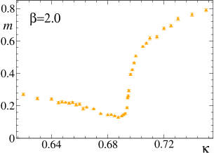
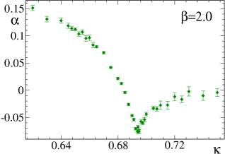
(a)	(b)
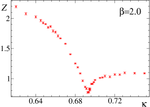
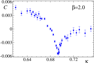
(c)	(d)

Figure 19: The fitting parameters for the propagator measured on $40^{3}$ at $\beta=2.0$ vs. $\kappa$.

as function of the hopping parameter $\kappa$. The optimal fit parameters have been found by minimizing $\chi^{2}/d.o.f$. Outside the critical region ($\kappa_{c}\approx 0.68$ – $0.70$) the propagator data are perfectly described by the simple fit ansatz (50). The quality of the fits is the same as in the $Q=1$ AHM Chernodub:2004yv , therefore we do not show a comparison of the measured data with the fits ansatz.

The propagator fit leads to a minimum of the photon mass (Fig. 19(a)). On the Higgs side of the transition the photon acquires its mass via the Higgs mechanism. The noted minimum could be explained similar to the $Q=1$ model via the interference between perturbative mass and Debye mass effects.

As shown in Fig. 19(b) the anomalous dimension $\alpha$ drops towards $\kappa_{c}$ and becomes negative near criticality within the used ansatz. It tends to zero from below at larger $\kappa$, deeper in the Higgs region. The strong wave function renormalization effects in the confining phase ($Z$ is much larger than one, see Fig. 19(c)) weaken towards the transition and $Z$ approaches a roughly constant value near one, deeper in the Higgs phase. For completeness, the contact term $C$ as function of $\kappa$ is shown in Fig. 19(d) as well.

In the critical region of the second order phase transition we observed that the propagator data for the smallest available lattice momenta seem to indicate a non-vanishing $p^{2}D(p^{2})$ for $p^{2}\to 0$, contrary to the used fit ansatz (as long as the fitted mass remains finite). For the worst observed case at $\kappa=0.695$ the smallest measured value for $p^{2}D(p^{2})$ lies roughly two times above the fit curve (at $p^{2}\approx 0.025$). The noticed deviation between data and fit curve is exclusively related only to the smallest lattice momenta. Nevertheless, the obtained values for $\chi^{2}/d.o.f.$ do not exceed 1.17 and do not differ significantly from the $\chi^{2}$ values outside the transition. More sophisticated parameterizations for the propagator and eventually measurements for still smaller momenta (larger lattices) are needed to clarify this problem what also might influence the actual values of our fit parameters. This, however, was beyond the scope of our present investigation.

V Conclusions

Summarizing, we have found that the compact Abelian Higgs model with doubly-charged matter field has a rich structure in terms of topological defects: monopoles and vortices. This structure has been outlined first by analytic considerations in the London limit and in the Villain representation. In particular, the topological character of confinement for $mod(q,Q)\neq 0$ via the Aharonov-Bohm (linking number) interaction has been pointed out.

Extending first results, obtained for a suitable finite-temperature regime of the model and published already in ref:U1Q2PLB , we could show by numerical simulation in the London limit, that the main property of the model, the existence of vortex clusters with monopoles attached to them is a generic feature of the model. This structure can explain that in the confining corner of the $\beta$-$\kappa$ phase diagram only odd-$q$ external charges are confined while even-$q$ charges suffer string breaking.

In the confinement phase we found that the vortex clusters are percolating. Both the length distribution of the vortex clusters and the monopole number distribution kept inside the clusters give rise to the definition of two order parameters, the “infrared densities” of monopoles and vortices. The infrared (percolating) component of the vortex network and the corresponding order parameters vanish in the Higgs phase.

For not too large lattice size at $T=0$ the phase transition is signalled also by the original gauge field variables, using for example the susceptibilities of the $q=1$ Polyakov loop on finite lattices (directly related to the loss of confinement for charge $q=1$ external charges). More quantitative description one can get from the susceptibilities of the monopole and vortex densities, and finally in terms of the two infrared order parameters. Different parts of the confining phase (high $\beta$ and small $\kappa$ on one hand and small $\beta$ and high $\kappa$ on the other) may differ in the detailed mechanism, being vortex driven (at low $\kappa$) or monopole driven (at low $\beta$).

We also have shown that the gauge boson propagator changes its character at the phase transition to the Higgs phase where it changes from confining to Yukawa type. There are remarkable differences from the $Q=1$ AHM. Using our simple parametrization (50) for the form factor $D(p^{2})$ we found that in the $Q=2$ case both the critical dimension $\alpha$, the photon renormalization function $Z$ and the contact term $C$ go through minima at the phase transition point, which is not the case for the $Q=1$ case. Moreover, in a vicinity of the phase transition the renormalization parameter $Z$ gets smaller than unity and the propagator can be described by a negative anomalous dimension contrary to the $Q=1$ case. We were not able to see the fitted gauge boson mass vanishing at pseudocriticality (eventually to be expected from the second order nature of the phase transition). So, this interesting behavior can be confirmed only using larger lattice sizes to access still lower lattice momenta and more sophisticated parameterizations for the propagator.

This study deepens our understanding of the phase transition in this model. It also further develops the paradigm for the cooperative role that monopoles and vortices play in non-Abelian gluodynamics. The physical picture – observed in the present study – has a close analogy with QCD (in 4D) where tight correlations between Abelian monopoles and center vortices have already been observed. The non-diagonal gluons are usually ignored after the Abelian projection (from the maximally Abelian gauge). In fact, they are charge-two matter field with respect to the remaining Abelian gauge symmetry. If these matter fields would be retained as dynamical, this might naturally lead to the formation of monopole sheets on vortex sheets, which in turn should be responsible for the permanent (in the pure gauge model) confinement of the fundamental charges (quarks) and for the flattening of the potential between the adjoint charges (“static gluons”).

- (1) E. H. Fradkin and S. H. Shenker, Phys. Rev. D 19, 3682 (1979); M. B. Einhorn and R. Savit, Phys. Rev. D 17, 2583 (1978); ibid. D 19, 1198 (1979).
- (2) G. Bhanot and B. A. Freedman, Nucl. Phys. B 190, 357 (1981).
- (3) N. Nagaosa and P. A. Lee, Phys. Rev. B 61, 9166 (2000); I. Ichinose, T. Matsui and M. Onoda, Phys. Rev. B 64, 104516 (2001).
- (4) H. Kleinert, F. S. Nogueira and A. Sudbø Phys. Rev. Lett. 88, 232001 (2002); A. Sudbø et al., ibid. 89, 226403 (2002).
- (5) Y. Fujita and T. Matsui, Proceedings of 9th International Conference on Neural Information Processing, pp. 1360. Edited by L.Wang, et al. (2002); cond-mat/0207023 .
- (6) M. N. Chernodub, R. Feldmann, E.-M. Ilgenfritz and A. Schiller, Phys. Lett. B 605, 161 (2005).
- (7) A. A. Abrikosov, Sov. Phys. JETP, 32 1442, (1957); H. B. Nielsen and P. Olesen, Nucl. Phys. B 61, 45 (1973).
- (8) A. M. Polyakov, Nucl. Phys. B 120, 429 (1977).
- (9) J. Fröhlich and T. Spencer, J. Stat. Phys. 24 (1981) 617; M. N. Chernodub, Phys. Rev. D 63, 025003 (2001).
- (10) N. Parga, Phys. Lett. B 107, 442 (1981); N. O. Agasian and K. Zarembo, Phys. Rev. D 57, 2475 (1998); M. N. Chernodub, E.-M. Ilgenfritz and A. Schiller, Phys. Rev. D 64, 054507 (2001); Phys. Rev. Lett. 88, 231601 (2002).
- (11) M. N. Chernodub, E.-M. Ilgenfritz and A. Schiller, Phys. Lett. B 547, 269 (2002); ibid. B 555, 206 (2003).
- (12) T. Suzuki, Nucl. Phys. Proc. Suppl. 30, 176 (1993); M. N. Chernodub and M. I. Polikarpov, “Abelian projections and monopoles”, in ”Confinement, duality, and nonperturbative aspects of QCD”, Ed. by P. van Baal, Plenum Press, p. 387, hep-th/9710205; R. W. Haymaker, Phys. Rept. 315, 153 (1999).
- (13) J. Greensite, Prog. Part. Nucl. Phys. 51, 1 (2003).
- (14) J. Ambjorn, J. Giedt and J. Greensite, JHEP 0002, 033 (2000); A. V. Kovalenko, M. I. Polikarpov, S. N. Syritsyn and V. I. Zakharov, hep-lat/0402017; V. I. Zakharov, in: H. Suganuma, N. Ishii, M. Oka, H. Enyo, T. Hatsuda, T. Kunihiro and K. Yazaki (Eds.), Color Confinement and Hadrons in Quantum Chromodynamics, World Scientific, Singapore, 2004, p. 112, hep-ph/0309301.
- (15) M. N. Chernodub, F. V. Gubarev and M. I. Polikarpov, Phys. Lett. B 416, 379 (1998); M. N. Chernodub, M. I. Polikarpov, A. I. Veselov and M. A. Zubkov, ibid. B 432 182, (1998).
- (16) R. Balian, J. M. Drouffe and C. Itzykson, Phys. Rev. D 11, 2098 (1975).
- (17) A. P. Gottlob and M. Hasenbusch, cond-mat/9305020; G. Kohring, R. E. Shrock and P. Wills, Phys. Rev. Lett. 57, 1358 (1986).
- (18) L. Del Debbio, M. Faber, J. Greensite and S. Olejník, Phys. Rev. D 55, 2298 (1997); R. Bertle, M. Faber, J. Greensite and S. Olejník, JHEP 9903, 019 (1999).
- (19) J. M. Kosterlitz, D. Thouless, J. Phys. C 6 1181, (1973).
- (20) V. L. Berezinsky, Sov. Phys. JETP 32, 493 (1971).
- (21) M. I. Polikarpov, U. J. Wiese and M. A. Zubkov, Phys. Lett. B 309, 133 (1993).
- (22) M. N. Chernodub, M. I. Polikarpov, M. A. Zubkov, Nucl. Phys. Proc. Suppl. 34, 256 (1994).
- (23) J. Ambjorn, J. Giedt and J. Greensite, JHEP 0002, 033 (2000); A. V. Kovalenko, M. I. Polikarpov, S. N. Syritsyn and V. I. Zakharov, hep-lat/0402017; V. I. Zakharov, hep-ph/0309301; hep-ph/0501011.
- (24) A. Hart and M. Teper, Phys. Rev. D 58, 014504 (1998); M. N. Chernodub and V. I. Zakharov, Nucl. Phys. B 669, 233 (2003).
- (25) M. N. Chernodub, K. Ishiguro, K. Kobayashi and T. Suzuki, Phys. Rev. D 69, 014509 (2004).
- (26) M. N. Chernodub, R. Feldmann, E.-M. Ilgenfritz and A. Schiller, Phys. Rev. D 70, 074501 (2004).