Abstract

An additional $Z_{6}$ symmetry hidden in the fermion and Higgs sectors of the Standard Model has been found recently[1]. A lattice regularization of the Standard Model was constructed that possesses this symmetry. In [2] we have reported our results on the numerical simulation of the electroweak sector of the model. In this paper we report our results on the numerical simulation of the full ($SU(3)\otimes SU(2)\otimes U(1)$ ) model. The phase diagram of the model has been investigated using static quark and lepton potentials. Various types of monopoles have been constructed. Their densities appear to be sensitive to the phase transition lines. Differences between the realizations of the Standard Model which do or do not possess the mentioned $Z_{6}$ symmetry, are discussed.

1 Introduction

Until recently it was thought that all the symmetries of the Standard Model (SM), which must be used when dealing with its discretization, are known. However, in [1] it was shown that there exists an additional $Z_{6}=Z_{2}\otimes Z_{3}$ symmetry in the fermion and Higgs sectors of the SM. It is connected to the centers $Z_{3}$ and $Z_{2}$ of the $SU(3)$ and $SU(2)$ subgroups. The gauge sector of the SM (in its discretized form) was redefined in such a way that it has the same naive continuum limit as the original one, while keeping the mentioned symmetry. The resulting model differs from the conventional SM via its symmetry properties. Therefore we expect, that nonperturbatively these two models may represent different physics.

Investigation of the electroweak sector of the SM with the additional $Z_{6}$ symmetry shows, that there are indeed certain differences between this discretization and the conventional one [2]. Namely, it has been found that the phase transition lines corresponding to the $U(1)$ and $SU(2)$ degrees of freedom join in a triple point, forming a common line. In contrast to this, in the conventional model the phase transition line corresponding to $SU(2)$ degrees of freedom has an endpoint and the transition becomes continuous in a certain region of coupling constants [4]. In this paper we report our results on the full SM (including $SU(3)$ degrees of freedom) and claim that the same phenomenon takes place here. Now the $SU(3)$, $SU(2)$ and $U(1)$ degrees of freedom are connected via their centers. This, in our opinion, is the reason why the phase transition lines corresponding to the phase transitions in pure $U(1)$ and $SU(2)$ models again join together forming a common line. It turns out that $SU(3)$ fields experience this common phase transition as well.

This paper is organized as follows. In the next section we summarize the formulation of the SM in terms of link variables and demonstrate the emergence of an additional $Z_{6}$ symmetry in its fermion and Higgs sectors. In Sect. 3 we detail the model with explicit $Z_{6}$ symmetry on the lattice, while in Sect. 4 we recall the definition of the maximal center projection. The next section contains the definitions of the quantities we measure on the lattice; it is followed by Sect. 6 where we show our numerical results. We end with a summary.

2 $Z_{6}$ symmetry in the Standard Model

In this section we remind the reader of what we call the additional $Z_{6}$ symmetry. The SM contains the following variables:

1. The gauge field ${\cal U}=(\Gamma,U,\theta)$, where

$$\Gamma\in SU(3),\quad U\in SU(2),\quad e^{i\theta}\in U(1),$$ (1)

realized as link variables on the lattice.

2. A scalar doublet

$$\Phi^{\alpha},\;\alpha=1,2.$$ (2)

3. Anticommuting spinor variables, representing leptons and quarks:

$$\left(\begin{array}[]{ccc}\nu_{e}&\nu_{\mu}&\nu_{\tau}\\ e&\mu&\tau,\end{array}\right),\quad\left(\begin{array}[]{ccc}u&c&t\\ d&s&b\end{array}\right).$$ (3)

The action has the form

$$S=S_{g}+S_{H}+S_{f},$$ (4)

where we denote the fermion part of the action by $S_{f}$, the pure gauge part is denoted by $S_{g}$, and the scalar part of the action by $S_{H}$.

In any lattice realization of $S_{H}$ and $S_{f}$ both these terms depend upon link variables $\cal U$ considered in the representations corresponding to quarks, leptons, and the Higgs scalar field, respectively. Therefore $\cal U$ appears in the combinations shown in the table.

$U\,e^{-i\theta}$	left-handed leptons
$e^{-2i\theta}$	right-handed leptons
$\Gamma\,U\,e^{\frac{i}{3}\theta}$	left-handed quarks
$\Gamma\,e^{-\frac{2i}{3}\theta}$	right-handed $d$, $s$, and, $b$ - quarks
$\Gamma\,e^{\frac{4i}{3}\theta}$	right-handed $u$, $c$, and, $t$ - quarks
$U\,e^{i\theta}$	the Higgs scalar field

Our observation is that all the listed combinations are invariant under the following transformations:

$$U \rightarrow Ue^{-i\pi N},$$

$$\theta \rightarrow \theta+\pi N,$$

$$\Gamma \rightarrow \Gamma e^{(2\pi i/3)N},$$ (5)

where $N$ is an arbitrary integer link variable. It represents a three-dimensional hypersurface on the dual lattice. Both $S_{H}$ and $S_{f}$ (in any realization) are invariant under the simultaneous transformations (5). This symmetry reveals the correspondence between the centers of the $SU(2)$ and $SU(3)$ subgroups of the gauge group.

After integrating out fermion and scalar degrees of freedom any physical variable should depend upon gauge invariant quantities only. Those are the Wilson loops: $\omega_{SU(3)}({\cal C})={\rm Tr}\Pi_{{\rm link}\in{\cal C}}\Gamma_{\rm link}$, $\omega_{SU(2)}({\cal C})={\rm Tr}\Pi_{{\rm link}\in{\cal C}}U_{\rm link}$, and $\omega_{U(1)}({\cal C})=\Pi_{{\rm link}\in{\cal C}}{\rm exp}(\frac{i}{3}\theta_{\rm link})$. Here $\cal C$ is an arbitrary closed contour on the lattice (with self - intersections allowed). These Wilson loops are trivially invariant under the transformation (5) with the field $N$ representing a closed three-dimensional hypersurface on the dual lattice. Therefore the nontrivial part of the symmetry (5) corresponds to a closed two-dimensional surface on the dual lattice that is the boundary of the hypersurface represented by $N$. Then in terms of the gauge invariant quantities $\omega$ the transformation (5) acquires the form:

$$\omega_{U(1)}({\cal C}) \rightarrow {\rm exp}(-i\mbox{\small$\frac{1}{3}$}\pi{\bf L}({\cal C},\Sigma))\,\omega_{U(1)}({\cal C})$$

$$\omega_{SU(2)}({\cal C}) \rightarrow {\rm exp}(i\pi{\bf L}({\cal C},\Sigma))\,\omega_{SU(2)}({\cal C})$$

$$\omega_{SU(3)}({\cal C}) \rightarrow {\rm exp}(i\mbox{\small$\frac{2}{3}$}\pi{\bf L}({\cal C},\Sigma))\,\omega_{SU(3)}({\cal C})$$ (6)

Here $\Sigma$ is an arbitrary closed surface (on the dual lattice) and ${\bf L}({\cal C},\Sigma)$ is the integer linking number of this surface and the closed contour $\cal C$. From (6) it follows, that the symmetry is of $Z_{6}$ type.

3 The model under investigation

It is obvious that the pure gauge-field part of the action in its conventional continuum formulation (or, say, in lattice Wilson formulation) is not invariant under (6). However, the lattice realization of the pure gauge field term of the action can be constructed in such a way that it also preserves the mentioned symmetry. For the reasons listed in [1] we consider it in the following form:

$$S_{g} = \beta\sum_{\rm plaquettes}\{2(1-\mbox{${\small\frac{1}{2}}$}{\rm Tr}\,U_{p}\cos\theta_{p})+$$ (7)

$$+\;(1-\cos 2\theta_{p})$$

$$+\;6[1-\mbox{${\small\frac{1}{6}}$}{\rm ReTr}\,\Gamma_{p}{\rm Tr}\,U_{p}{\rm exp}(i\theta_{p}/3)]$$

$$+\;3[1-\mbox{${\small\frac{1}{3}}$}{\rm ReTr}\,\Gamma_{p}{\rm exp}(-2i\theta_{p}/3)]$$

$$+\;3[1-\mbox{${\small\frac{1}{3}}$}{\rm ReTr}\,\Gamma_{p}{\rm exp}(4i\theta_{p}/3)]\},$$

where the sum runs over the elementary plaquettes of the lattice. Each term of the action Eq. (7) corresponds to a parallel transporter along the boundary $\partial p$ of plaquette $p$. The corresponding plaquette variables constructed of lattice gauge fields are $U_{p}=\omega_{SU(2)}(\partial p)\,,\Gamma_{p}=\omega_{SU(3)}(\partial p)\,$, and $\theta_{p}={\rm Arg}\,\omega_{U(1)}(\partial p)$.

The potential for the scalar field is considered in its simplest form [2] in the London limit, i.e., in the limit of infinite bare Higgs mass. After fixing the unitary gauge we obtain:

$$S_{H} = \gamma\sum_{xy}[1-Re(U^{11}_{xy}e^{-i\theta_{xy}})].$$ (8)

The following variables are (naively) considered as creating a photon, $Z$ boson, and $W$ boson respectively:

$$A_{xy} = A^{\mu}_{x}\;=\,[{\rm Arg}U_{xy}^{11}+\theta_{xy}]\,{\rm mod}\,2\pi,$$

$$Z_{xy} = Z^{\mu}_{x}\;=\,[{\rm Arg}U_{xy}^{11}-\theta_{xy}]\,{\rm mod}\,2\pi,$$

$$W_{xy} = W^{\mu}_{x}\,=\,U_{xy}^{12}e^{i\theta_{xy}}.$$ (9)

Here, $\mu$ represents the direction $(xy)$. After fixing the unitary gauge the electromagnetic $U(1)$ symmetry remains:

$$U_{xy} \rightarrow g^{\dagger}_{x}U_{xy}g_{y},$$

$$\theta_{xy} \rightarrow \theta_{xy}+\alpha_{y}/2-\alpha_{x}/2,$$ (10)

where $g_{x}={\rm diag}(e^{i\alpha_{x}/2},e^{-i\alpha_{x}/2})$. The fields $A$, $Z$, and $W$ transform as follows:

$$A_{xy} \rightarrow A_{xy}+\alpha_{y}-\alpha_{x},$$

$$Z_{xy} \rightarrow Z_{xy},$$

$$W_{xy} \rightarrow W_{xy}e^{-i\alpha_{x}}.$$ (11)

We consider our model in quenched approximation, i.e., we neglect the effect of virtual fermion loops. Therefore the particular form of $S_{f}$ is not of interest for us at this stage.

In order to extract physical information from the $SU(3)$ fields in a particulary simple way we use the so-called indirect Maximal Center Projection (see, for example, [5, 6]).

4 The Maximal Center Projection.

The Maximal Center Projection makes the link matrix $\Gamma$ as close as possible to the elements of the center $Z_{3}$ of $SU(3)$: $Z_{3}=\{{\rm diag}(\mathrm{e}^{(2\pi i/3)N},\mathrm{e}^{(2\pi i/3)N},\mathrm{e}^{(2\pi i/3)N}\}$, where $N\in\{1,0,-1\}$. The procedure works as follows.

First, make the functional

$$Q_{1}=\sum_{\mathrm{links}}(|\Gamma_{11}|+|\Gamma_{22}|+|\Gamma_{33}|)$$ (12)

maximal with respect to the gauge transformations $\Gamma_{xy}\rightarrow g^{\dagger}_{x}\Gamma_{xy}g_{y}$, thus fixing the Maximal Abelian gauge. As a consequence every link matrix becomes almost diagonal.

Secondly, to make this matrix as close as possible to the center of $SU(3)$, make the phases of the diagonal elements of this matrix maximally close to each other. This is done by minimizing the functional

$$Q_{2} = \sum_{\mathrm{links}}\{[1-\cos({\rm Arg}(\Gamma_{11})-{\rm Arg}(\Gamma_{22}))]+[1-\cos({\rm Arg}(\Gamma_{11})-{\rm Arg}(\Gamma_{33}))]$$ (13)

$$+\;[1-\cos({\rm Arg}(\Gamma_{22})-{\rm Arg}(\Gamma_{33}))]\}.$$

with respect to the gauge transformations. This gauge condition is invariant under the central subgroup $Z_{3}$ of $SU(3)$.

In our model $SU(3)$ fields are connected with the $U(1)$ and $SU(2)$ fields via the center of the gauge group. Therefore, instead of the center vortices and center monopoles we define various kinds of monopole - like fields. The definitions of these fields includes the following integer-valued link variable $N$ (defined after fixing the Maximal Center gauge):

$$N_{xy}=0 {\rm if} ({\rm Arg}(\Gamma_{11})+{\rm Arg}(\Gamma_{22})+{\rm Arg}(\Gamma_{33}))/3\in\;]-\pi/3,\pi/3],$$

$$N_{xy}=1 {\rm if} ({\rm Arg}(\Gamma_{11})+{\rm Arg}(\Gamma_{22})+{\rm Arg}(\Gamma_{33}))/3\in\;]\pi/3,\pi],$$

$$N_{xy}=-1 {\rm if} ({\rm Arg}(\Gamma_{11})+{\rm Arg}(\Gamma_{22})+{\rm Arg}(\Gamma_{33}))/3\in\;]-\pi,-\pi/3].$$ (14)

In other words, $N=0$ if $\Gamma$ is close to $1$, $N=1$ if $\Gamma$ is close to $\mathrm{e}^{2\pi i/3}$ and $N=-1$ if $\Gamma$ is close to $\mathrm{e}^{-2\pi i/3}$.

Next, we define the following link fields

$$C^{1}_{xy} = \,\left[\frac{2\pi}{3}N_{xy}+{\rm Arg}U_{xy}^{11}+\frac{1}{3}\theta_{xy}\right]\,{\rm mod}\,2\pi,$$

$$C^{2}_{xy} = \,\left[\frac{2\pi}{3}N_{xy}-\frac{2}{3}\theta_{xy}\right]\,{\rm mod}\,2\pi,$$

$$C^{2}_{xy} = \,\left[\frac{2\pi}{3}N_{xy}+\frac{4}{3}\theta_{xy}\right]\,{\rm mod}\,2\pi.$$ (15)

These fields correspond to the last three terms of Eq. (7). Their construction comes from the representation of $\Gamma$ as a product of $\exp((2\pi i/3)N)$ and $V$, where $V$ is the $SU(3)/Z_{3}$ variable $({\rm Arg}(V_{11})+{\rm Arg}(V_{22})+{\rm Arg}(V_{33}))/3\in\;]-\pi/3,\pi/3]$. Thus $\Gamma=\exp((2\pi i/3)N)V$. We expect, that (7) suppresses $V_{\rm plaq}$ and $C^{i}_{\rm plaq},i=1,2,3$ while the fields $N$, $\frac{\theta}{3}$, and $U_{11}$ (being considered independently of each other) are expected to be disordered. This assumption is justified by the numerical simulations.

5 Quantities to be measured

We investigated five types of monopoles. The monopoles, which carry information about colored fields are extracted from $C^{i}$:

$$j_{C^{i}}=\frac{1}{2\pi}{}^{*}d([dC^{i}]{\rm mod}2\pi).$$ (16)

(Here we used the notations of differential forms on the lattice. For a definition of those notations see, for example,  [7].)

Pure $U(1)$ monopoles, corresponding to the second term in (7), are extracted from $2\theta$:

$$j_{2\theta}=\frac{1}{2\pi}{}^{*}d([d2\theta]{\rm mod}2\pi).$$ (17)

The electromagnetic monopoles, corresponding to the first term in (7), are:

$$j_{A}=\frac{1}{2\pi}{}^{*}d([dA]{\rm mod}2\pi).$$ (18)

The density of the monopoles is defined as follows:

$$\rho=\left\langle\frac{\sum_{\rm links}|j_{\rm link}|}{4L^{4}}\right\rangle,$$ (19)

where $L$ is the lattice size. To understand the dynamics of external charged particles, we consider the Wilson loops defined in the fermion representations listed above (in the table):

$${\cal W}^{\rm L}_{\rm lept}(l) = \langle{\rm Re}{\rm Tr}\,\Pi_{(xy)\in l}U_{xy}e^{-i\theta_{xy}}\rangle,$$

$${\cal W}^{\rm R}_{\rm lept}(l) = \langle{\rm Re}\Pi_{(xy)\in l}\,e^{-2i\theta_{xy}}\rangle,$$

$${\cal W}^{\rm L}_{{\rm quarks}}(l) = \langle{\rm Re}\Pi_{(xy)\in l}\,\Gamma_{xy}\,U_{xy}\,e^{\frac{i}{3}\theta_{xy}}\rangle,$$

$${\cal W}^{\rm R}_{{\rm down}\,{\rm quarks}}(l) = \langle{\rm Re}\Pi_{(xy)\in l}\,\Gamma_{xy}\,e^{-\frac{2i}{3}\theta_{xy}}\rangle,$$

$${\cal W}^{\rm R}_{{\rm up}\,{\rm quarks}}(l) = \langle{\rm Re}\Pi_{(xy)\in l}\,\Gamma_{xy}\,e^{\frac{4i}{3}\theta_{xy}}\rangle.$$ (20)

Here $l$ denotes a closed contour on the lattice. We consider the following quantity constructed from the rectangular Wilson loop of size $a\times t$:

$${\cal V}(a)=\lim_{t\rightarrow\infty}\frac{{\cal W}(a\times t)}{{\cal W}(a\times(t+1))}.$$ (21)

A linear behavior of ${\cal V}(a)$ would indicate the existence of a charge - anti charge string with nonzero tension.

6 Numerical results

In our calculations we investigated lattices $L^{4}$ for $L=6$, $L=12$, and $L=16$ with symmetric boundary conditions.

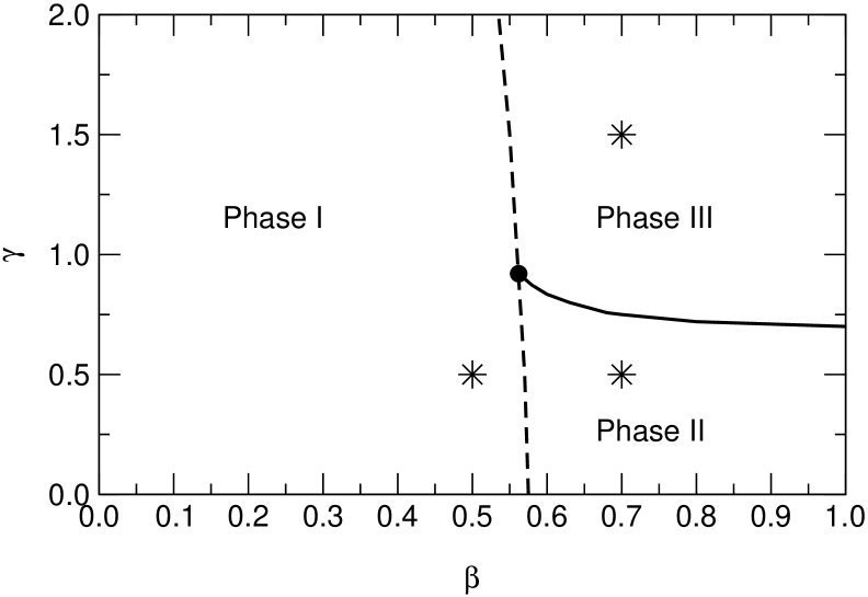
Figure 1: The phase diagram of the model in the $(\beta,\gamma)$-plane.

We summarize our qualitative results in the phase diagram represented in Fig. 1. The model contains three phases. The first one (I) is a phase, in which the dynamics of external leptons is confinement - like, i.e. is similar to that of external charges in QCD with dynamical fermions. In the second phase (II) the behavior of left-handed leptons is confinement-like, while for right-handed ones it is not. The last one (III) is the Higgs phase, in which no confining forces between leptons are observed at all. In all three phases there is the confinement of all external quark fields (left quarks, right up quarks, right down quarks).

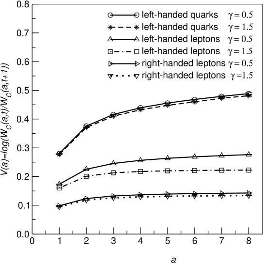
Figure 2: ${\cal V}_{L}(a)$ calculated at $\beta=0.7$. Here the potentials are extracted from ${\cal W}^{\rm L}_{{\rm quarks}}$(left - handed quarks), ${\cal W}^{\rm L}_{{\rm lept}}$ (left - handed leptons), and ${\cal W}^{\rm R}_{{\rm lept}}$ (right - handed leptons).

This is illustrated by Figs. 2, in which we show ${\cal V}(a)$ extracted from the Wilson loops Eq. (20) at two typical points that belong to phases II ($\gamma=0.5$) and III ($\gamma=1.5$) of the model (the behavior of all potentials in the phase I is confinement - like). We represent here the potential for only one colored Wilson loop, i.e. for ${\cal W}^{\rm L}_{{\rm quarks}}$, because the string tension extracted from the other two potentials coincides with the string tension extracted from the potential represented in the figure within the errors. This is, of course, exactly what we have expected: string tensions for different types of quarks are equal to each other. Thus, the potential, extracted from the colored fields, possesses linear behavior in all phases, indicating appearance of confinement of quarks.

By making a linear fit to the lepton potentials at values $a\geq 5$ we found that only in the case of left-handed leptons the value of the string tension is much larger than its statistical uncertainty in phase II. For left-handed leptons in the Higgs phase and right-handed leptons in both phases, the uncertainty in the values of the string tension turns out to be larger than about 24% of its value. In these cases we do not consider the string tension to be significantly different from zero. However, as for QCD with dynamical fermions or the $SU(2)$ fundamental Higgs model [10, 13], these results do not mean that confinement of leptons occurs. The charge - anti charge string must be torn by virtual charged scalar particles, which are present in the vacuum due to the Higgs field. Thus ${\cal V}(a)$ may be linear only at sufficiently small distances, while starting from some distance it must not increase, indicating the breaking of the string. Unfortunately the accuracy of our measurements does not allow us to observe this phenomenon in detail.

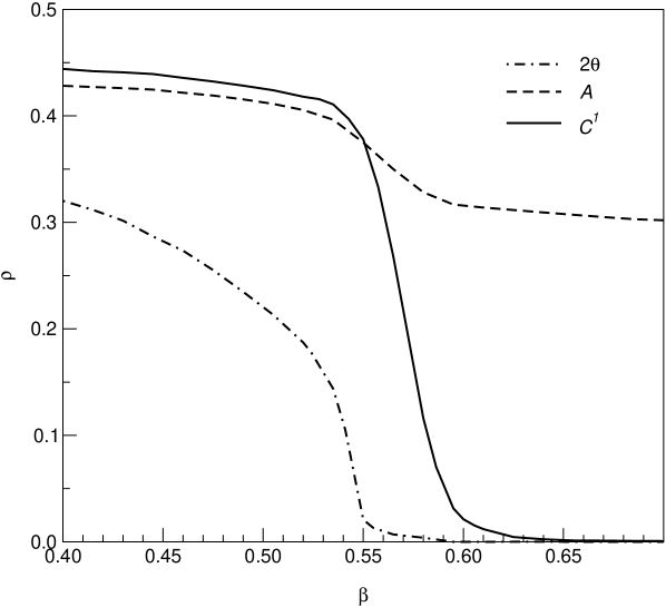
Figure 3: The monopole densities (constructed of the link fields $A,2\theta$, and $C^{1}$) versus $\beta$ at fixed $\gamma=0.5$.

The connection between the properties of monopoles and the phase structure of the model is illustrated by Figs. 3, which shows the monopole density versus $\beta$ at fixed $\gamma=0.5$. Again we represent here only one type of the three monopoles, which have colored origin. Namely, we consider $j_{C^{1}}$. (Behavior of the others is similar.) One can see, that the density of the $2\theta$ - monopoles as well as $C^{1}$ - monopoles falls sharply in phase II, while the electromagnetic monopole density does not.

We note here, that according to our measurements the electromagnetic monopole density falls to zero while shifting from phases I to III. The colored monopoles and $2\theta$ - monopole densities fall sharply in the phase III as well. Thus monopoles composed of colored fields feel the phase transition, which are due, according to our intuition, to the $U(1)$ variables. This happens again because the $Z_{6}$ symmetry binds $U(1)$ variables with the center of the $SU(3)$ subgroup of the gauge group.

As in [2] we mention here that the $SU(2)$ fundamental Higgs model, has a similar phase structure as our model, except for the absence of the phase transition line between phases I and II. In the latter model it was shown that different phases are actually not different. This means that the phase transition line ends at some point and the transition between two states of the model becomes continuous. Thus one may expect that in our model the phase transition line between phases I and III ends at some point. However, we do not observe this for the considered values of couplings.

In our model both phase transition lines join in a triple point, forming a common line. This is, evidently, the consequence of the mentioned additional symmetry that relates $SU(2)$ , $U(1)$, and $SU(3)$ excitations. The same picture, of course, does not emerge in the conventional $SU(3)\otimes SU(2)\otimes U(1)$ gauge – Higgs model: its $SU(2)\otimes U(1)$ part was investigated, for example, in [4]. As for the $SU(3)$ gauge theory, it has no phase transition at finite $\beta$ and zero temperature at all.

7 Conclusions

We summarize our results as follows:

1. We performed a numerical investigation of the quenched lattice model that respects the additional symmetry.

2. The lattice model contains three phases. In the first phase the potential between static leptons is confinement-like. In the second phase the confining forces are observed, at sufficiently small distances, between the left-handed external leptons. The last one is the Higgs phase, where there are no confinement - like forces between static leptons at all.

3. Investigation of the monopoles constructed of colored fields shows that colored fields feel the phase transition lines.

4. In all phases of the model we observe confinement of quarks. The string tensions for different kinds of quarks are equal to each other.

5. The main consequence of the emergence of the additional symmetry is that the phase transition lines corresponding to the $SU(2)$ and $U(1)$ degrees of freedom join in a triple point forming a common line. This reflects the fact that the $SU(2)$ and $U(1)$ excitations are related due to the mentioned symmetry. The same situation does not occur in the conventional $SU(2)\otimes U(1)$ gauge - Higgs model [4].

So, we have found a qualitative difference between the conventional discretization and the discretization that respects the invariance under the transformations given in Eq. (6).

In order to illustrate other possible differences let us consider the problem of constructing the operator which creates a glueball in the $Z_{6}$ invariant version of the lattice SM. Here we cannot use the conventional expression

$${\cal O}_{c}=\left(1-\frac{1}{3}{\rm Re}\,{\rm tr}\,\Gamma_{\rm plaq}\right)$$ (22)

as it is not invariant under our $Z_{6}$ symmetry. Instead we may use $Z_{6}$ - invariant expressions like

$${\cal O}=\left(1-\frac{1}{3}{\rm Re}\,{\rm tr}\{\Gamma_{\rm plaq}e^{-\frac{2i}{3}\theta_{\rm plaq}}\}\right)-\frac{1}{9}(1-{\rm cos}\,2\theta_{\rm plaq})$$ (23)

In the naive continuum limit the above expressions (22) and (23) coincide. In a similar way the naive continuum limit of the action (7) coincides with that of the conventional lattice SM action for the appropriate choice of coupling constants.

However, this coincidence does not mean necessarily, that either the models themselves or the correlators of operators (22) and (23) lead to the same results. Let us recall here two precedents, i.e., two similar situations, where the coincidence of the naive continuum limits does not lead to the same physics.

The first example is the massless lattice fermion. One may compare Wilson fermions with the simplest direct discretization of the Dirac fermion action[11]. These two actions differ from each other by a term which naively vanishes in the continuum limit. However, the corresponding models are not identical from the physical point of view. Namely, the second one contains $15$ additional fermion species while in the Wilson formulation all of them acquire infinite mass and disappear in the continuum limit. This phenomenon of fermion doubling is widely discussed in the literature. It is worth mentioning that another difference between these two formulations is the absence of exact chiral symmetry in the Wilson formulation and its appearance in the naive discretization.

The second example is the pure nonabelian gauge theory. If we would discretize its form written in terms of gauge potentials losing the exact gauge invariance, the resulting lattice model would have the same naive continuum limit as the conventional lattice gluodynamics, which is written in terms of link matrices. However, in such a definition of lattice gauge theory confinement is lost[12].

In the two examples of lattice models considered above, which have the same naive continuum limit but different symmetry properties, finally lead to different physics. Exactly the same situation may be present in our case, where the naive continuum limit of the two lattice realizations of the SM is the same, while only one formulation is $Z_{6}$ invariant.

Another argument in favor of the point of view that these two models are indeed different, comes from the direct consideration of how continuum physics emerges in the lattice SM. Namely, there are indications [8, 9] that several kinds of singular field configurations may survive in the continuum limit of nonabelian lattice gauge models. If so, the conventional action of the lattice SM and the action (7) may appear to be different when approaching the continuum for singular field configurations of various kinds.

We are grateful to F.V. Gubarev and Yu.A. Simonov for useful discussions. A.I.V. and M.A.Z. kindly acknowledge the hospitality of the Department of Physics and Astronomy of the Vrije Universiteit, where part of this work was done. We also appreciate I. Gogoladze and R. Shrock, who have brought to our attention references [3] and [4] respectively. This work was partly supported by RFBR grants 03-02-16941, 05-02-16306, 04-02-16079, and PRF grant for leading scientific schools N 1774.2003.2, by Federal Program of the Russian Ministry of Industry, Science, and Technology No 40.052.1.1.1112.

References

- [1] B.L.G. Bakker, A.I. Veselov, and M.A. Zubkov, Phys. Lett. B 583, 379 (2004);
- [2] B.L.G. Bakker, A.I. Veselov, and M.A. Zubkov, Yad. Fiz. , (2005);
-
[3]
K.S. Babu, I. Gogoladze, and K. Wang, Phys. Lett. B 570, 32 (2003);
K.S. Babu, I. Gogoladze, and K. Wang, Nucl. Phys. B 660, 322 (2003); - [4] R. Shrock, Phys. Lett. B 162, 165 (1985); Nucl. Phys. B 267, 301 (1986).
- [5] J. Greensite, Prog. Part. Nucl. Phys. 51 (2003) 1
- [6] B.L.G. Bakker, A.I. Veselov, and M.A. Zubkov, Phys. Lett. B 471 (1999) 214
- [7] M.I. Polikarpov, U.J. Wiese, and M.A. Zubkov, Phys. Lett. B 309, 133 (1993).
- [8] B.L.G. Bakker, A.I. Veselov, and M.A. Zubkov, Phys. Lett. B 544, 374 (2002);
-
[9]
F.V. Gubarev and V.I. Zakharov, hep-lat/0211033;
F.V. Gubarev, A.V. Kovalenko, M.I. Polikarpov, S.N. Syritsyn, and V.I. Zakharov, Phys. Lett. B 574 136 (2003) - [10] I. Montvay, Nucl. Phys. B269, 170 (1986).
-
[11]
N.B. Nielsen and M. Ninomiya,
Nucl. Phys. B 185, 20 (1981); ibid, 173;
M. Lüscher, Phys. Lett. B 428, 342 (1998);
H. Neuberger, Phys. Lett. B 417, 141 (1998)
-
[12]
A. Patrascioiu, E. Seiler, and I.O. Stamatescu,
Phys. Lett. B 107, 364 (1981);
E. Seiler, I.O. Stamatescu, and D. Zwanziger, Nucl. Phys. B 239, 177 (1984);
Y. Yotsuyanagi, Phys. Lett. B 135, 141 (1984);
K. Cahill, S. Prasad, R. Reeder, and B. Richter,
Phys. Lett. B 181, 333 (1986);
K. Cahill, Phys. Lett. B 231, 294 (1989) -
[13]
M. Gurtler, E.M. Ilgenfritz, and A. Schiller, Phys. Rev. D 56, 3888
(1997);
B. Bunk, E.M. Ilgenfritz, J. Kripfganz, and A. Schiller, Nucl. Phys. B 403, 453 (1993);
M.N. Chernodub, F.V. Gubarev, E.M. Ilgenfritz, and A. Schiller, Phys. Lett. B 434, 83 (1998);
M.N. Chernodub, F.V. Gubarev, E.M. Ilgenfritz, and A. Schiller, Phys. Lett. B 443, 244 (1998).