An example of optimal field cut in lattice gauge perturbation theory

Abstract

We discuss the weak coupling expansion of a one plaquette $SU(2)$ lattice gauge theory. We show that the conventional perturbative series for the partition function has a zero radius of convergence and is asymptotic. The average plaquette is discontinuous at $g^{2}=0$. However, the fact that $SU(2)$ is compact provides a perturbative sum that converges toward the correct answer for positive $g^{2}$. This alternate method amounts to introducing a specific coupling dependent field cut, that turns the coefficients into $g$-dependent quantities. Generalizing to an arbitrary field cut, we obtain a regular power series with a finite radius of convergence. At any order in the modified perturbative procedure, and for a given coupling, it is possible to find at least one (and sometimes two) values of the field cut that provide the exact answer. This optimal field cut can be determined approximately using the strong coupling expansion. This allows us to interpolate accurately between the weak and strong coupling regions. We discuss the extension of the method to lattice gauge theory on a $D$-dimensional cubic lattice.

I Introduction

Lattice gauge theory incorporates essential features of the strong interactions at short distance (asymptotic freedom) and large distance (confinement). Expansions in $1/\beta=g^{2}/2N$ and $\beta$ usually provide good approximations for the average value of gauge invariant quantities in the limit of small or large $\beta$. However, calculations in the intermediate region often require a numerical approach.

There exists a general method for calculating Wilson’ s or Polyakov’s loops in powers of $1/\beta$ Heller and Karsch (1985) in pure $SU(N)$ gauge theories (see Ref. Capitani (2003) for a more complete set of references on lattice perturbation theory).

Much effort has been devoted calculating

$$P\equiv\left\langle(1/N_{p})\sum_{p}(1-(1/N)ReTrU_{p})\right\rangle$$ (1)

where $U_{p}$ denotes the usual product of links along a $1\times 1$ plaquette and $N_{p}$ the number of plaquettes. $P$ can be obtained by taking the derivative with respect to $\beta$ of the free energy density. Exact calculations of the coefficients of $P$ up to order 3 in $1/\beta$ Allés et al. (1994) and numerical calculations at order 8 Di Renzo et al. (1995) and 10 Di Renzo and Scorzato (2001) are available. The accuracy of the weak and strong coupling expansions at successive orders is shown in Fig. 1 for $SU(3)$ in 4 dimensions. The figure makes clear that in the region $5<\beta<6$, none of the expansions (in powers of $\beta$ or $1/\beta$) is accurate. Unfortunately, this region is precisely the “scaling window” where one can extract information relevant to the continuum limit. In addition, the convergence of the weak coupling expansion is not completely understood. The analysis of the numerical series Horsley et al. (2002) may suggest the possibility of a finite radius of convergence (the center of the circle being $g^{2}=0$). This possibility is not expected on general grounds and is in contradiction with the discontinuity of $P$ when $g^{2}$ changes sign Li and Meurice (2005, 2004). We are not aware of any independent argument in favor of a finite radius of convergence, and the most likely outcome is that the factorial growth of the series takes over at higher order. In Ref. 6, this order is estimated to be approximately 25, which is out of reach of numerical calculations.

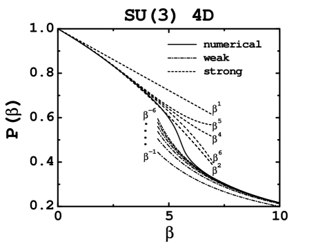
Figure 1: $P$ versus $\beta$ for $SU(3)$ in 4 dimensions. The solid line represents the numerical values; the dashed lines on the left, successive orders in the strong coupling expansion; the dot-dash lines on the right, successive orders in the weak coupling expansion.

In this article, we show that for a $SU(2)$ lattice gauge model on a single plaquette, the weak coupling expansion is asymptotic (has zero radius of convergence), but that it is possible to modify the perturbative procedure in order to get a convergent sum, which is an “expansion” in powers of $1/\beta$ but with $\beta$-dependent coefficients, that is accurate even in the strong coupling region. This work is motivated by recent results obtained in the case of scalar field theory Meurice (2002); Kessler et al. (2004) where the answer for similar questions in the case of nontrivial models can be guessed correctly by considering a single site integral. This is briefly reviewed in Sec. II. The main point is that the large order behavior of perturbation theory is related to large field configurations and that by cutting-off these configurations appropriately, we can obtain a series that converges to a value exponentially close to the exact one (for instance, errors of order ${\rm e}^{-\lambda\phi^{4}_{max}}$ for the simple integral discussed in Ref. Kessler et al. (2004)). Hereafter, we follow the same path for lattice gauge theories.

The $SU(2)$ model is introduced in Sec. III where we also discuss its connection to Bessel functions. It is worth noting that for compact groups, there are no large field contributions and consequently, the factorial growth of the perturbative series comes from adding the tails of integration, as done in asymptotic analysis of integrals Bleistein and Handelsman (1986) and in the conventional procedure used in lattice perturbation theoryHeller and Karsch (1985). This is explained in Section IV. In many quantum problems, the lack of convergence can be traced to the behavior of the model at negative coupling (see, however, Ref. Bender and Boettcher (1998) for a proper definition). This question has been discussed for lattice gauge models in 4 dimensions Li and Meurice (2005). In Sec. V, we argue that there should be an essential singularity at zero coupling for the one plaquette model. In Sec. VI, we show that the regular perturbation series (with the integration tails added) misses “instanton effects” of the form $\beta^{-1}{\rm e}^{-2\beta}$.

In Sec. VII, we propose to modify the conventional perturbative method by introducing a field cut. With this modification, the series converges toward a value which in general is different than the exact one. However, at a given order in the weak coupling expansion, it is possible to pick an optimal field cut such that for a given coupling the answer is exact. For the integral studied in this article, we found at least one solution at every order. This is not necessarily the case in general. For the integral studied in Ref. Kessler et al. (2004), we were able to prove that no such solution exists at odd order and that we could only minimize the error in that case. In Sec. VIII, we use the strong coupling expansion to determine approximately this optimal field cut. In this approach, the field cut is given as a power series in $\beta$. A numerical study indicates that this series has a finite radius of convergence which increases with the order in $1/\beta$ considered. The method that we propose allows us to interpolate between the weak and strong coupling region. This is depicted in Fig. 2, which is the prototype of what we expect to accomplish in general. In the conclusions, we consider the implementation of the method for $D$-dimensional models and discuss three practical ways to calculate the modified coefficients.

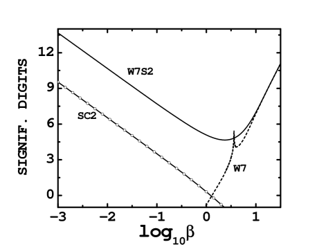
Figure 2: Number of significant digits for the $SU(2)$ one plaquette integral, at order 7 in the weak coupling (dotted line W7), at order 2 in the strong coupling (empty circles SC2) and at order 7 of the modified perturbative method proposed here with an optimal field cut determined pointwise using the strong coupling expansion at order 2 (solid line W7S2).

II Motivations

A common challenge for quantum field theorists consists in finding accurate methods in regimes where existing expansions break down. In the renormalization group language, this amounts to finding acceptable interpolations for the flows in intermediate regions between fixed points. A discussion of this question for lattice gauge theories can be found in Refs. Kogut et al. (1979); Kogut and Shigemitsu (1980). In the case of scalar field theory, the weak coupling expansion is unable to reproduce the exponential suppression of the large field configurations operating at strong coupling. This problem can be cured Meurice (2002) by introducing a large field cutoff $\phi_{max}$ which eliminates Dyson’s instability. One is then considering a slightly different problem, however a judicious choice of $\phi_{max}$ can be used to reduce or eliminate Kessler et al. (2004) the discrepancy with the original problem (i. e., the problem with no field cutoff). This optimization procedure can be approximately performed using the strong coupling expansion and naturally bridges the gap between the weak and strong coupling expansions.

The study of the simple integral

$$\int_{-\infty}^{+\infty}d\phi e^{-\frac{1}{2}\phi^{2}-\lambda\phi^{4}}\neq\sum_{0}^{\infty}\frac{(-\lambda)^{l}}{l!}\int_{-\infty}^{+\infty}d\phi e^{-\frac{1}{2}\phi^{2}}\phi^{4l}$$ (2)

provides a good understanding about the role of large field configurations in the perturbative series. It helps identifying general features of the the effect of a field cut. In particular, the dependence of the accuracy of the modified perturbative series on the coupling and the field cut, is qualitatively very similar for the integral, the anharmonic oscillator and the hierarchical model in 3 dimensions (see the similarity among the three parts of Fig. 2 in Meurice (2002)).

In order to generalize this procedure to gauge theory, we will first consider the simplest possible gauge model, namely the one plaquette integral

$$Z(\beta,N)=\int\prod_{l\in p}dU_{l}{\rm e}^{-\beta(1-\frac{1}{N}ReTrU_{p})}\ ,$$ (3)

After fixing the gauge so that $U=1$ on three sides of the plaquette, $Z$ becomes an integral over a single link

$$Z(\beta,N)=\int dU{\rm e}^{-\beta(1-\frac{1}{N}ReTrU)}$$ (4)

For an arbitrary gauge fixing prescription, $TrU$ becomes $Tr(U(g)U)$ with $g$ arbitrary and $Z$ is $g$-independent by virtue of the invariance of the Haar measure $dU$. This integral and its moments appear in the strong coupling expansion Kogut et al. (1979); Munster and Weisz (1981); Falcioni et al. (1981); Smit (1982) and in the mean field treatment Drouffe and Zuber (1983) of $SU(N)$ gauge theories. In the one plaquette model,

$$P=-\frac{d}{d\beta}{\rm ln}Z\ .$$ (5)

The accuracy of successive orders in the $\beta$ and $1/\beta$ described in the following sections is shown in Fig. 3 that can be compared with Fig. 1.

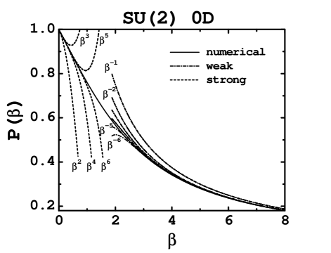
Figure 3: $P$ versus $\beta$ for $SU(2)$ on one plaquette. The solid line represents the numerical values; the dashed lines on the left, successive orders in the strong coupling expansion; the dot-dash lines on the right, successive order in the weak coupling expansion.

III The model considered here

In the following, we specialize the discussion to the case $N=2$ for which the Haar measure is very simple. From now on, the reference to $N$ will be dropped and we will use the notation $Z(\beta)$ for $Z(\beta,2)$. The explicit form is:

$$Z(\beta)=\frac{1}{\pi}\int_{0}^{2\pi}d\omega\sin^{2}(\omega/2){\rm e}^{-\beta(1-\cos(\omega/2))}\ .$$ (6)

Setting $u={\rm cos}(\omega/2)$,

$$Z(\beta)=\frac{2}{\pi}\int_{-1}^{1}du\sqrt{1-u^{2}}{\rm e}^{-\beta(1-u)}$$ (7)

and one recognizes from Eq. (8.431) of Ref. Gradshteyn and Ryzhik (1980) that the integral can be expressed in terms of the modified Bessel function $I_{1}$:

$$Z(\beta)=2{\rm e}^{-\beta}I_{1}(\beta)/\beta$$ (8)

Using the Taylor expansion Eq. (8.445) in Ref. Gradshteyn and Ryzhik (1980), we can write

$$2I_{1}(\beta)/\beta=\sum_{l=0}^{\infty}\frac{1}{l!\Gamma(l+2)}(\beta/2)^{2l}\ .$$ (9)

As in the case of the integral of Eq. (2), the presence of the factorial at the denominator implies that the strong coupling expansion (in powers of $\beta=4/g^{2}$) converges over the entire complex plane.

IV The weak coupling expansion

Assuming $\beta>0$, we set $t=\beta(1-u)$ in Eq. (7) yields

$$Z(\beta)=(2/\beta)^{3/2}\frac{1}{\pi}\int_{0}^{2\beta}dtt^{1/2}{\rm e}^{-t}\sqrt{1-(t/2\beta)}$$ (10)

If we expand the square root in the integral and exchange the sum and the integral (the validity of this procedure will be discusssed in Sec. VII), we obtain a converging sum:

$$Z(\beta)=(\beta\pi)^{-3/2}2^{1/2}\sum_{l=0}^{\infty}A_{l}(2\beta)\beta^{-l}\ ,$$ (11)

with

$$A_{l}(x)\equiv 2^{-l}\frac{\Gamma(l+1/2)}{l!(1/2-l)}\int_{0}^{x}dt{\rm e}^{-t}t^{l+1/2}\ ,$$ (12)

The convergence of the sum in Eq. (11) can be established from the bounds

$$\frac{{\rm e}^{-2\beta}}{l+3/2}(2\beta)^{l+3/2}<\int_{0}^{2\beta}dt{\rm e}^{-t}t^{l+1/2}<\frac{1}{l+3/2}(2\beta)^{l+3/2}\ ,$$ (13)

and the fact that $\Gamma(l+1/2)/l!<1$ for $l\geq 1$. (This is true for $l=1$ and can be proved by induction multiplying the inequality by $(l+1/2)/(l+1)<1$). Consequently, the sum converges at the same rate as $\sum l^{-2}$. Note that as in the case of the ground state of the quantum mechanical double well, the first term is positive but all the remaining terms are negative.

Obviously, Eq. (11) is not a power series in $\beta^{-1}$ since the “coefficients” $A_{l}(2\beta)$ are $\beta$-dependent. We can now obtain the conventional asymptotic expansion by two different methods. The first one consists in adding the tails to the integrals in Eq. (12), or in other words by replacing the incomplete gamma function by the gamma function. This is a standard procedure in asymptotic expansions of integrals Bleistein and Handelsman (1986).

On then obtain the asymptotic expansion

$$Z(\beta)\sim(\beta\pi)^{-3/2}2^{1/2}\times$$ (14)

$$\sum_{l=0}^{\infty}(2\beta)^{-l}\frac{(\Gamma(l+1/2))^{2}(l+1/2)}{l!(1/2-l)},$$

The terms of this sum now grow like $l!/2^{l}$ and the series is asymptotic. As all the signs are negative for $l\geq 1$, the Borel transform has singularities on the positive real axis.

It is instructive to rederive the expansion of Eq. (14) by following the steps of lattice perturbation theory Heller and Karsch (1985). We first set $\omega=gA$ in Eq. (6) and expand the action and the Haar measure in powers of $g$. This leaves us with the integral of a power series in $g$ over the range 0 to $2\pi/g$ for $A$. The asymptotic series (14) is then recovered by letting the range of integration go to infinity. As the two methods amount to calculate the coefficients with different variables of integration, we obtain the same series, as can be checked explicitly up to high order. We emphasize that in lattice gauge theory with compact groups, there are no large field contributions. It is only for practical reasons that the tails of integration are added. In the one plaquette example, calculating $A_{l}(2\beta)$ instead of $A_{l}(\infty)$ is a very minor problem, however, this is a technical challenge in the case on a $D$-dimensional lattice

V Behavior at negative $\beta$

From the integral representation Eq. (7), the change $\beta\rightarrow-\beta$ can be made by changing $u\rightarrow-u$ and multiplying by ${\rm e}^{2\beta}$. This implies,

$$Z(-\beta)={\rm e}^{2\beta}Z(\beta)\ ,$$ (15)

and

$$P(\beta)+P(-\beta)=2$$ (16)

A similar equation Li and Meurice (2005) can be found for a $SU(2)$ pure gauge model on a cubic lattice. Since $lim_{\beta\rightarrow+\infty}P(\beta)=0$, the limits $g^{2}\rightarrow 0^{\pm}$ differ by 2 and a converging series in $g$ about 0 is impossible.

The discontinuity in the values of $P$ near $g^{2}=0$ appears in a simpler model where the integration over $SU(2)$ is replaced by a sum over the two elements of its center:

$$Z_{center}=\sum_{U=\pm\openone}{\rm e}^{-\beta(1-\frac{1}{2}ReTrU)}=1+{\rm e}^{-2\beta}\ .$$ (17)

This implies

$$P_{center}=\frac{2}{1+{\rm e}^{2\beta}}\ .$$ (18)

The center model satisfies Eqs. (15) and (16). Note that Eq. (17) makes clear that $Z_{center}$ has an essential singularity at $g=0$. The asymptotic behavior of $P_{center}$ at large $|\beta|$ in the complex plane is $2(1-{\rm e}^{2\beta}+\dots)$ if $Re\beta<0$, and $2{\rm e}^{-2\beta}+\dots$, if $Re\beta>0$, with Stokes lines running along the imaginary axis.

This simplified example makes clear that the usual perturbation series is obtained by making modifications of order ${\rm e}^{-2\beta}$ (the effect of the tails of integration). We now proceed to estimate the order ${\rm e}^{-2\beta}$ corrections to the integral over the whole $SU(2)$.

VI Accuracy of regular perturbation theory

In the study of scalar models Meurice (2002), we have shown that if we plot the accuracy of perturbative series at successive orders, an envelope setting the boundary of the accuracy that can be reached at any order using the usual perturbation theory appears. In the case of the quantum mechanical double-well, this envelope coincides very precisely with the instanton effect. We expect the limitation in accuracy to be of the general form $g^{A}{\rm e}^{-B/g^{2}}$. For the model considered here, the limitation of accuracy has this generic form and we will see that the effect is of order $\beta^{-1}{\rm e}^{-2\beta}$.

For $\beta$ not too small, the low orders the asymptotic series Eq. (14) overestimate $Z$. As we let the order increase, the series crosses the true value and then start to grossly underestimate the true value. At each order, there is a special value of $\beta$ for which the truncated series coincides with the exact answer. This explains the “spikes” seen in Fig. 4.

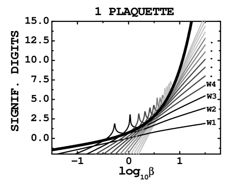
Figure 4: Number of correct significant digits as a function of $\beta$ at successive orders of the regular perturbative series Eq. (14) for $Z(\beta)$. As the order increases from 1 to 15, the curves ($W1,\ W2,\dots)$ get lighter. The thick solid line is ${\rm log}_{10}(\beta^{-1}{\rm e}^{-2\beta}/Z)$.

If we assume that for a particular value of $\beta$, the converging sum, Eq. (11) with the integrals running from 0 to $2\beta$, truncated at order $K$ is a good approximation of $Z(\beta)$, then the error $\delta Z(\beta,K)$ made by using the regular perturbative series, Eq. (14) with the integrals running from 0 to $\infty$, truncated at the same order, is in good approximation

$$\delta Z(\beta,K)\simeq(\beta\pi)^{-3/2}2^{1/2} \times$$

$$\sum_{l=0}^{K}(2\beta)^{-l}\frac{\Gamma(l+1/2)}{l!(1/2-l)}\int_{2\beta}^{\infty} dt {\rm e}^{-t}t^{l+1/2}\ ,$$ (19)

Integrating by parts, dropping terms of order $\beta^{-1}$ and summing the resulting series, we obtain

$$\delta Z(\beta,K)\approx A_{K}{\rm e}^{-2\beta}\beta^{-1}2\pi^{-3/2}\ ,$$ (20)

with

$$A_{K}=-\sum_{l=0}^{K}\frac{\Gamma(l-1/2)}{l!}\ .$$ (21)

The coefficient $A_{K}$ slowly decreases when $K$ increases. For instance, $A_{5}=0.872\dots$, $A_{10}=0.624\dots$. In the limit of large $K$, $A_{K}$ becomes zero. This comes from the resummation

$$\sum_{l=1}^{\infty}\frac{\Gamma(l-1/2)}{l!}=\int_{0}^{\infty}dtt^{-3/2}(1-{\rm e}^{-t})=2\pi^{1/2}\ ,$$ (22)

which is exactly the $l=0$ term. In practice, when the order is not too large, $\beta^{-1}{\rm e}^{-2\beta}$ is a good order of magnitude estimate for the envelope discussed above as can be seen in Fig. 4.

VII Modified model with an arbitrary field cut

In this section,we consider a modified partition function $Z(\beta,t_{max})$ where the integration range of Eq. (10) takes a fixed, $\beta$-independent, value $t_{max}$. When $t_{max}<2\beta$, the Taylor series for the square root converges absolutely and uniformly over the whole range of integration. It is thus justified to interchange the sum and the integral and we have

$$Z(\beta,t_{max})=(\beta\pi)^{-3/2}2^{1/2}\sum_{l=0}^{\infty}A_{l}(t_{max})\beta^{-l}\ .$$ (23)

The original partition function as expressed in Eq. (11) is obtained by taking the limit $t_{max}\rightarrow 2\beta$. Since the integral with upper boundary $t_{max}$ is obviously continuous in that limit and since we can use the $l^{-2}$ suppression to prove the continuity of the sum, the validity of Eq. (23) extends which justifies Eq. (11). If $t_{max}>2\beta$, the sum diverges and the integral is ill-defined. The regular perturbation series is obtained by taking the limit $t_{max}\rightarrow\infty$. In the graphs, we use the notation “WK” for the truncation of the regular perturbative series at order $K$. One should however keep in mind that, for instance in $W7$, the last term is of order $(1/\beta)^{7+3/2}$ due to the prefactor $\beta^{-3/2}$ in Eq. (23).

Eq. (23) is now a regular series in $(1/\beta)$. It has a finite radius of convergence. In order to calculate this radius, we notice that for large $l$, $\int_{0}^{t_{max}}dtt^{l}$ gets most of its contribution from the region between $t_{max}(1-1/l)$ and $t_{max}$. Consequently, one can replace ${\rm e}^{-t}t^{1/2}$ by ${\rm e}^{-t_{max}}t_{max}^{1/2}$ without affecting the asymptotic behavior of the coefficients of the series. If we perform this change directly in the integral Eq. (10), the integral can be calculated explicitly. One can then conclude that $Z(\beta,t_{max})$ has a non-analytical part proportional to $(1-(t_{max}/2\beta))^{3/2}$. The series defined by Eq. (23) converges if $(1/\beta)\leq(2/t_{max})$. Numerical studies of the series with conventional estimators confirm this argument. Note that the finite radius of convergence of the series Eq. (refeq:mod) is not in disagreement with the discontinuity of the original model at $1/\beta=0$, because this series coincides with the original model only when $(1/\beta)=(2/t_{max})$.

Can a truncation of the series of Eq. (23) at order $K$ be a good approximation of the original integral Eq. (6)? The answer depends on $K$, $t_{max}$ and $\beta$. It is clear that if $K$ is large enough and $\beta$ slightly above $2/t_{max}$, then one should get a reasonable approximation. This statement is confirmed by Fig. 5 where the accuracy of Eq. (23) with $t_{max}=8$ truncated at orders 1 to 15 is displayed as a function of $\beta$. In this particular case, the values of $\beta\geq 4$ are within the radius of convergence. As the order increases, the spikes in this region (the right half of the Fig. 5) move toward 4. In addition, there is another set of spikes, outside the radius of convergence (on the left half of the Fig. 5) and moving in the opposite direction when the order increases.

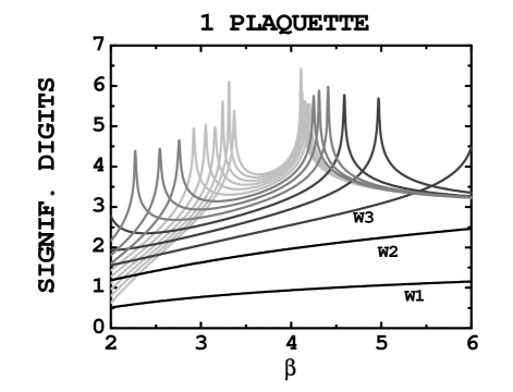
Figure 5: Number of correct significant digits as a function of $\beta$ for a fixed cut $t_{max}=8$. As the order increases from 1 to 15 ($W1,\ W2,\dots$), the curves become lighter.

A more global information regarding the location of the spikes is displayed in Fig. 6. It shows that the “second solution”, outside the radius of convergence, disappears beyond some critical value of $\beta$. As the order in the weak coupling increases, both solutions get closer to the $t_{max}=2\beta$ line.

Figure 6: Location of the exact matching between the series Eq. (23) at order 6, 7 and 8 and $Z(\beta)$ in the $\beta$-$t_{max}$ plane. The dashed lines represent the solution within the radius of convergence and the empty circles the other solution.

VIII Optimization

In this section, we discuss an approximate method to find the optimal value of $t_{max}$ corresponding to a given order $K$ and a given value of $\beta$. In a general situation, we do not know accurately the value of the quantity that we are calculating (the equivalent of $Z$ here). Consequently, we need to find an approximation that allows us to consistently estimate this quantity and the way its order $K$ approximation changes with the field cutoff in order to impose an approximate matching condition. For this purpose, we will use the strong coupling expansion (power series in $\beta$) which provides information complementary to the weak coupling. Now, the crucial point is that the field cut allows us to control the $(1/\beta)$ in the integral Eq. (10), because (except in the exponential) all the factor $(1/\beta)$ appear together with a factor $t$. In other words, except for the exponential,it is a function of $t/\beta$.

We would like to match the the strong coupling expansion

$$Z(\beta)=1-\beta+(5/8)\beta^{2}+\dots$$ (24)

discussed in Sec. III, with the truncated expansion of Eq. (23) which can be rewritten as

$$\pi^{-3/2}2\sum_{l=0}^{K}\frac{\Gamma(l+1/2)}{l!(1/2-l)}\int_{0}^{t_{max}/\beta}ds{\rm e}^{-s\beta}(s/2)^{l+1/2}\ .$$

The control of $s=t/\beta$ can be achieved by imposing that $t_{max}/\beta$ is approximately constant. We can then improve order by order in $\beta$ by setting

$$(t_{max}/\beta)=c_{0}(K)+c_{1}(K)\beta+\dots$$ (25)

The only non-trivial part is to solve the zeroth order (in $\beta$) equation

$$F_{K}(c_{0}(K))=1\ ,$$ (26)

with

$$F_{K}(x)=-4(\pi)^{-3/2}\sum_{l=0}^{K}\frac{\Gamma(l-1/2)(x/2)^{l+3/2}}{l!(l+3/2)}\ .$$ (27)

We have checked that for $K$ going from 1 to 40, Eq. (26) has exactly two solutions on the positive real axis with one solution on each side of 2. As $K$ increases, the 2 roots get closer. They should coalesce at 2 in the large $K$ limit. This follows from the fact that $F_{\infty}(2)=1$ and $F^{\prime}_{\infty}(2)=0$ (as can be shown by using the the same method as for Eq. (22)). The higher order coefficients $c_{l}(K)$ corresponding to each of the two solutions at order 0 can then be found by solving linear equations. This procedure provides an approximate value of the optimal $t_{max}$ which apparently converges toward the correct numerical value. This is illustrated in Fig. 7.

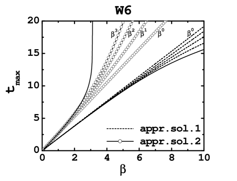
Figure 7: Approximate locations in the $(\beta,t_{max})$ plane of the matching between the order 6 weak coupling expansion and $Z(\beta)$. The two solid lines are the two numerical solutions at that order (as in Fig. 6). The dash line (empty circles) represent the first (second) approximate solutions at order $0,\dots,4$ in $\beta$.

If we plug the two approximate values of $t_{max}$ of Eq. (25) in Eq. (23) truncated at order $K$, we obtain approximate values of $Z(\beta)$. The accuracy of this procedure is displayed in Fig. 8 in the case $K=6$. It appears clearly that the first solution (the one within the radius of convergence with $t_{max}<2\beta$) is significantly more accurate than the other solution (with $t_{max}>2\beta$). Similar features were observed for $K$ up to 20.

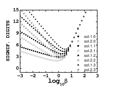
Figure 8: Significant digits obtained from Eq. (23) truncated at order 6 using $t_{max}/\beta$ at order 0 (squares), 1 (circles), 2 (triangles) and 3 (stars). The first solution with $t_{max}<2\beta$ is showed with filled symbols, while the second solution is showed with empty symbols.

We can now compare the accuracy of the method proposed here with the weak and strong coupling expansions. The case $K=6$ is displayed in Fig. (9). In the weak coupling region ($\beta>10$) the accuracy of our procedure merges with the regular perturbation series. In the strong coupling region ($\beta<0.1$), our procedure is more accurate than the regular expansion in powers of $\beta$ by several significant digits. As $\beta\rightarrow 0$, the accuracy of our procedure with $t_{max}/\beta$ determined at order $m$ in $\beta$ increases at the same rate as the regular strong coupling expansion at order $m$ in $\beta$ maintaining the difference in accuracy approximately constant. In the intermediate region where none of the conventional expansions work well (except at the perturbative spike), our procedure maintains a very good accuracy interpolating smoothly between the two regimes.

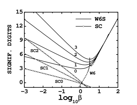
Figure 9: Significant digits obtained from Eq. (23) truncated at order 6 using the first solution for $t_{max}/\beta$ at order 0 to 3 compared to the weak coupling expansion at order 6 (dotted line W6) and the strong coupling expansion at order 0 to 2 (empty circles SC)

IX Asymptotic behavior of $c_{l}(K)$

In this section, we study empirically the asymptotic behavior of the coefficients $c_{l}(K)$ appearing in the expansion of $t_{max}/\beta$ Eq. (25). At fixed $K$ large $l$ , Fig. 10 suggests that

$$c_{l}(K)\propto(G(K))^{l}\ .$$ (28)

In addition, it appears that $G(K)$ decreases with $K$ approximately like $1/K$. This behavior implies a finite radius convergence $G(K)^{-1}$ for the $\beta$ expansion in Eq. (25), increasing linearly with $K$. This is good news for the interpolation between the weak and strong coupling region since as we increase the weak order $K$, we increase the range of validity in $\beta$.

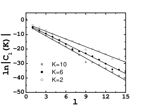
Figure 10: $\ln|c_{l}(K)|$ versus $l$ for $K=2,\ 6\ ,10$.

The large-$K$ behavior of $c_{l}(K)$ has also been studied numerically. The results for $l$ up to 5 are shown in Fig. 11.

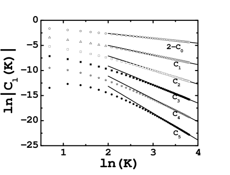
Figure 11: $\ln|c_{0}(K)-2|$ versus $\ln K$; $\ln|c_{l}(K)|$ versus $\ln K$ for $l=1,\dots 5$.

At fixed $l$ large $K$ , the linear fits used in Fig. 11 suggest that

$$c_{0}(K)\simeq 2+O(1/K)\ ,$$ (29)

and

$$c_{l}(K)\propto K^{-l-1+\alpha(l)}\ ,$$ (30)

for $l>0$, with $\alpha(l)$ small. This behavior is expected, since as the order increases, we are getting close to the exact expansion Eq. (11) with $t_{max}=2\beta$ ($c_{0}=2,\ c_{l}=0$ for $l>0$). The values of $\alpha(l)$ decrease when we reduce the set of points fitted to larger values of $K$. If we use $K=35$ to 45 for the fit, we have approximately $\alpha(l)\simeq l/10$.

X Conclusions

We have shown that for the one-plaquette model, the introduction of a properly chosen field cut can provide a high accuracy in regions where the usual perturbative method is not accurate. The strong coupling expansion provides an efficient way to determine the optimal cut and interpolate between the small and the large $\beta$ regions. Apparently, the accuracy of the calculations improves whenever we increase the order in either the weak or the strong coupling expansion. Given these positive results, we are compelled to implement the method in the case of lattice gauge theory on a $D$ dimensional cubic lattice. Two steps are necessary. First, we need to define the theory with a field cut (the analog of Eq. (10) with $2\beta$ replaced by $t_{max}$). Second, we need to expand relevant quantities such as $P$ for the modified theory in powers of $1/\beta$ (the analog of Eq. (23)). Note that in the calculation of P using a perturbative series, the complex zeroes of Z will play an important role. This question remains to be examined in detail.

The implementation of the first step is straightforward. One can insert 1 in the partition function in the following way:

$$1=\prod_{p}\int_{0}^{t_{max}}dt_{p}\delta(1-(1/N)ReTr(U_{p})-t_{p})\ .$$ (31)

If we could perform the integration over the $U_{link}$, we would get an effective theory for the new variables $t_{P}$. Note that the procedure is gauge invariant since $TrU_{p}$ is. The “size” of a configuration can be defined in several ways. For instance, we could use the value of $Max_{p}\left\{t_{p}\right\}$ or $(1/N_{p})\sum_{p}t_{p}$ to decide if we have a large or a small field configuration. We can then order the configurations according to the chosen indicator. Given a (sufficiently large) set of Monte Carlo configurations, one can define the expectation values with a cut by averaging only over configurations for which the chosen indicator is below a certain value. The correlations between the two size indicators mentioned above are now being studied for $SU(3)$ in 4 dimensions.

The implementation of the second step requires technologies that are now being developed in the scalar case. As it seems only possible to make analytical calculations for small or large field cuts, numerical methods seem unavoidable. For the purpose of independent verification, it is important to consider different methods. We are presently working on three different approaches:

1. The conventional approach Heller and Karsch (1985) but with the $A_{\mu}^{a}$ having a finite range of integration. This type of approach works well in the scalar case Li and Meurice

2. The stochastic approach Di Renzo et al. (1995) where $A_{\mu}^{a}$ is expanded as power series in $1/\beta$. For the lowest order field, the implementation of a cut is obvious but not for higher order fields. This problem is being considered with simple examples.

3. Fits from numerical data at large $\beta$. This method J. Cook and Meurice allowed to extract at least 2 coefficients of conventional perturbation. As we mentioned above, it is easy to implement the field cut with Monte Carlo methods. The advantage of this method is that it does not require the use of the Campbell-Baker-Hausdorff (for a short review see Ref. Zachos ) formula.

We expect that the use of theses three methods will allow us to contruct perturbative series with a finite radius of convergence as above. We hope that this radius of convergence will be sufficiently large to reach the scaling window. Ultimately, we expect to be able to replace the numerical calculation of the coefficients by approximate analytical formulas, as it seems possible to do in the case of the anharmonic oscillator Li and Meurice .