Unquenched quark propagator in Landau gauge

Abstract

We present an unquenched calculation of the quark propagator in Landau gauge with 2+1 flavors of dynamical quarks. We use configurations generated with an improved staggered (“Asqtad”) action by the MILC collaboration. This quark action has been seen to have excellent rotational symmetry and scaling properties in the quenched quark propagator. Quenched and dynamical calculations are performed on a $20^{3}\times 64$ lattice with a nominal lattice spacing of $a=0.125$ fm. The matched quenched and dynamical lattices allow us to investigate the relatively subtle sea quark effects, and even in the quenched case the physical volume of these lattices gives access to lower momenta than our previous study. We calculate the quark mass function and renormalization function for a variety of valence and sea quark masses.

I Introduction

Quantum Chromodynamics is widely accepted as the correct theory of the strong interactions and the quark propagator is its most basic quantity. In the low momentum region it exhibits dynamical chiral symmetry breaking (which cannot be derived from perturbation theory) and at high momentum it can be used to extract the running quark mass Bowman:2004xi . In lattice QCD, quark propagators are tied together to calculate hadron masses and other properties. Lattice gauge theory provides a way to calculate the quark propagator directly, providing access to quantities such as operator product expansion (OPE) condensates Arriola:2004en . In turn, such a calculation can provide technical insight into lattice gauge theory simulations.

The systematic study of the quark propagator on the lattice has also provided fruitful interaction with other approaches to hadron physics, such as instanton phenomenology Diakonov:2002fq , chiral quark models Arriola:2003bs and Dyson-Schwinger equation studies Bhagwat:2003vw ; Alkofer:2003jj . The lattice is a first principles approach and has provided valuable constraints for model builders. In turn, such alternative methods can provide feedback on regions that are difficult to access directly on the lattice, such as the deep infrared and chiral limits.

The quark propagator has previously been studied using Clover Skullerud:2000un ; Skullerud:2001aw , staggered Bowman:2002bm ; Bowman:2002kn and Overlap Bonnet:2002ih ; Zhang:2003fa actions. For a review, see Ref. Bowman:Springer . All these actions have different systematic errors and the combination of these studies has given us an excellent handle on the possible lattice artifacts. In every case, however, they have been performed in the quenched approximation and have been restricted to modest physical volumes.

In this paper we report first results for the quark propagator including dynamical quark effects. We use configurations generated by the MILC Collaboration Bernard:2001av available from the Gauge Connection nersc . These use “Asqtad”, ${\cal O}(a^{2})$ improved staggered quarks Orginos:1999cr , giving us access to relatively light sea quarks. In the quenched approximation, the quark propagator for this action has excellent rotational symmetry and is well behaved at large momenta Bowman:2004xi . We use quenched and dynamical configurations at the same lattice spacing and volume, which enables us to observe the relatively subtle effects of unquenching. These lattices are also somewhat larger than those of previous studies, giving us access to smaller momenta.

II Details of the calculation

The quark propagator is gauge dependent and we work in the Landau gauge for ease of comparison with other studies. Landau gauge is a smooth gauge that preserves the Lorentz invariance of the theory, so it is a popular choice. It will be interesting to repeat this calculation for the Gribov-copy free Laplacian gauge, and this is left for a future study.

The MILC configurations were generated with the ${\cal O}(a^{2})$ one-loop Symanzik-improved Lüscher–Weisz gauge action Luscher:1984xn . The dynamical configurations use the Asqtad quark action, an ${\cal O}(a^{2})$ Symanzik-improved staggered fermion action. They have two degenerate light fermions, for the $u$ and $d$ quarks, and a heavier one for the strange quark. We explore a variety of light quark masses, with the bare strange quark mass fixed at $ma=0.05$, or $m$ = 79 MeV for $a$ = 0.125 fm Davies:2003ik . In all cases the Asqtad action is also used for the valence quarks. The values of the coupling and the bare sea-quark masses are matched such that the lattice spacing is held constant. This means that all systematics are fixed; the only variable is the addition of quark loops. The simulation parameters are summarized in Table 1.

Table 1: Lattice parameters used in this study. The dynamical configurations each have two degenerate light (up/down) quarks and a heavier (strange) quark. The lattice spacing is $a=0.125(3)$ fm, where the uncertainty reflects the variation of $a$ over the set of lattices considered in this analysis. Bare light quark masses $ma=0.01,0.02,0.03,0.04$ correspond to masses of $16-63$ MeV. The bare strange quark mass is $ma=0.05$ or $79$ MeV.

	Dimensions	$\beta$	Bare Quark Mass	# Config
1	$20^{3}\times 64$	8.00	quenched	265
2	$20^{3}\times 64$	6.76	$16$ MeV, $79$ MeV	203
3	$20^{3}\times 64$	6.79	$32$ MeV, $79$ MeV	249
4	$20^{3}\times 64$	6.81	$47$ MeV, $79$ MeV	268
5	$20^{3}\times 64$	6.83	$63$ MeV, $79$ MeV	318

On the lattice, the bare propagator $S(a;p^{2})$ is related to the renormalized propagator $S^{\text{ren}}(\mu;p^{2})$ through the renormalization constant

$$S(a;p^{2})=Z_{2}(a;\mu)S^{\text{ren}}(\mu;p^{2}).$$ (1)

In the continuum limit, Lorentz invariance allows one to decompose the full quark propagator into Dirac vector and scalar pieces

$$S^{-1}(p^{2})=iA(p^{2})\gamma\cdot p+B(p^{2})$$ (2)

or, alternatively,

$$S^{-1}(p^{2})=Z^{-1}(p^{2})[i\gamma\cdot p+M(p^{2})],$$ (3)

where $M(p^{2})$ and $Z(p^{2})$ are the nonperturbative mass and wave function renormalization functions, respectively. Asymptotic freedom implies that, as $p^{2}\rightarrow\infty$, $S(p^{2})$ reduces to the free propagator

$$S^{-1}(p^{2})\rightarrow i\gamma\cdot p+m,$$ (4)

up to logarithmic corrections. The mass function $M$ is renormalization point independent and for $Z$ we choose throughout this work the renormalization point as 3 GeV.

The tree-level quark propagator with the Asqtad action has the form

$$S^{-1}(p)=i\sum_{\mu}\overline{\gamma}_{\mu}q(p_{\mu})+m,$$ (5)

where $q(p_{\mu})$ is the kinematic momentum given by Bowman:2002bm

$$q_{\mu}\equiv\sin(p_{\mu})\bigl{[}1+\frac{1}{6}\sin^{2}(p_{\mu})\bigr{]}.$$ (6)

The $\overline{\gamma}_{\mu}$ form a staggered Dirac algebra. Having identified the kinematic momentum, we define the mass and renormalization functions by

$$S^{-1}(p)=Z^{-1}(q)\Bigl{[}i\sum_{\mu}{(\overline{\gamma}_{\mu})}q_{\mu}(p_{\mu})+M(q)\Bigr{]}.$$ (7)

Complete details of the extraction of the mass and renormalization functions from the Asqtad propagator are described in the appendix.

III Quenched Results

First we compare our quenched results to some previously published data obtained on a smaller lattice Bowman:2002kn . All the data illustrated in the following are cylinder cut Bonnet:2001uh . This removes points most susceptible to rotational symmetry breaking, making the data easier to interpret. As is well known, the definition of lattice spacing in a quenched calculation is somewhat arbitrary, and indeed the quoted estimate for our smaller ensemble is not consistent with that published for the MILC configurations. We determined a consistent value of the lattice spacing by matching the gluon propagator calculated on the old ensemble to that of the new ensemble Bowman:2004jm . This procedure yields a new nominal lattice spacing of $a=0.105$ fm and physical volume of $1.7^{3}\times 3.4~{}\text{fm}^{4}$ for the old lattices. Examining the quark propagator on the two quenched ensembles, shown in Fig. 1, we see that the agreement is excellent. This indicates that both finite volume and discretization effects are small. The flattening in the deep infrared of both scalar functions is a long-standing prediction of DSE studies Bhagwat:2003vw .

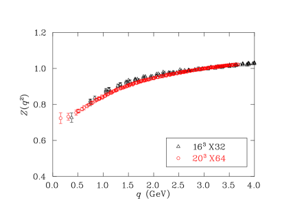
Figure 1: Comparison of quenched wave-function renormalization and mass functions at approximately the same bare quark mass. The quark propagator from the $20^{3}\times 64$ lattice with lattice spacing $a=0.125$ fm at $m=47$ MeV (open circles) is compared with the previously published quark propagator from a $16^{3}\times 32$ lattice with lattice spacing $a=0.105$ fm at $m=45$ MeV (full triangles). The renormalization point for $Z(q^{2})$ is set at $q$ = 3 GeV.

We show results for the larger quenched lattice for a variety of bare quark masses in Fig. 2. Once again we see that for quark masses less than or approximately equal to that of the strange quark, the lowest momentum point of the mass function is insensitive to quark mass.

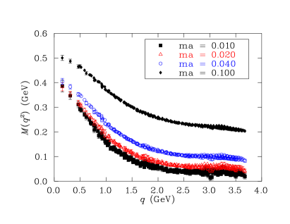
Figure 2: The quenched renormalization function (top) and mass function (bottom) for a selection of quark masses, including $ma=0.100$, about twice the strange quark mass. The renormalization point for $Z(q^{2})$ is set at $q$ = 3 GeV.

IV Effects of Dynamical Quarks

Here we compare the scalar functions for the quenched and dynamical propagators. For a given bare mass, the running mass depends upon both the number of dynamical quark flavors and their masses. To make the most appropriate comparison we select a bare quark mass for the quenched case ($ma=0.01$) and interpolate the dynamical mass function so that it agrees with the quenched result at the renormalization point, $q=3$ GeV. The results are shown in Fig. 3.

The dynamical case does not differ greatly from the quenched case. For the renormalization functions, there is no discernible difference between the quenched and unquenched cases. However the mass functions do reveal the effects of dynamical quarks. Dynamical mass generation is suppressed in the presence of dynamical quarks relative to that observed in the quenched case. This is in accord with expectations as the dynamical quark loops act to screen the strong interaction.

Further comparisons can be made in the chiral limit. In Fig. 4 both quenched and dynamical data have been extrapolated to zero bare quark mass by a fit linear in the quark mass. In the dynamical case, the extrapolation is limited to the case where the valence and sea quark masses match for the light quarks. While the results are qualitatively similar to those of Fig. 3, increased separation is observed in the generation of dynamical mass. As discussed above, for a given bare quark mass, the running mass is larger in full QCD than in quenched QCD.

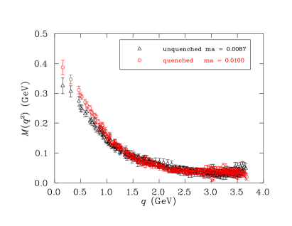
Figure 3: Comparison of the unquenched (full QCD) and quenched quark propagator for non-zero quark mass. The mass function for the unquenched dynamical-fermion propagator has been interpolated so that it agrees with the quenched mass function for $ma=0.01$ at the renormalization point, $q$ = 3 GeV. For the unquenched propagator this corresponds to a bare quark mass of $ma=0.0087$.

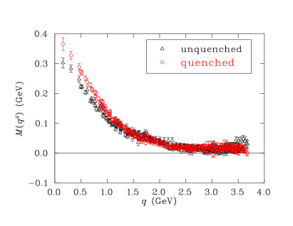
Figure 4: Comparison of the unquenched (full QCD) and quenched quark propagator in the chiral limit. The renormalization function is renormalized at $q$ = 3 GeV. Whereas little difference is observed in the renormalization function, the mass functions indicates that dynamical mass generation is suppressed by the addition of quark loops.

Fig. 5 shows the mass and renormalization functions in the dynamical case for a variety of quark masses. Here the valence quark masses and the light sea quark masses are matched. The results show that the renormalization function is insensitive to the bare quark masses studied here. The results for the mass function are ordered as expected with the larger bare quark masses, $m$, giving rise to a larger mass function.

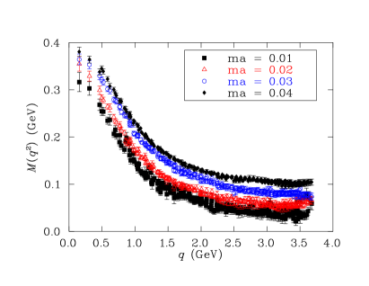
Figure 5: Renormalization (top) and mass (bottom) functions for four different quark masses in full QCD, where the valence and light-sea masses are matched. The wave-function renormalization function $Z$ is renormalized at $q$ = 3 GeV.

Finally, we comment on the approach to the chiral limit. In Fig. 6 we show the mass function for five different momenta plotted as a function of the bare quark mass. The momenta considered include the lowest momentum of 0.155 GeV and 0.310, 0.495, 0.700 and 0.993 GeV to explore momentum dependent changes in the approach to the chiral limit. At larger momenta, the mass function is observed to be proportional to the bare quark mass. However, at small momenta, nonperturbative effects make this dependence more complicated. For example, a recent Dyson-Schwinger study predicts a downward turn as the bare mass approaches zero Bhagwat:2003vw .

For the lowest momentum points, nonlinear behavior is indeed observed. For the quenched case, curvature in an upward direction is revealed as the chiral limit is approached, leading to the possibility of a larger infrared mass function for the lightest quark mass, despite the reduction of the input bare quark mass. In contrast, a hint of downward curvature is observed for the most infrared points of the full QCD mass function as the chiral limit is approached. It is interesting that the nature of the curvature depends significantly on the chiral dynamics of the theory which are modified in making the quenched approximation. Similar behavior is observed in the hadron mass spectrum where the coefficients of chiral nonanalytic behavior can change sign in moving from quenched QCD to full QCD Leinweber:2003ux ; Young:2002cj .

Figure 6: The chiral limit approach of the mass function for selected momenta. Results from quenched QCD simulations are illustrated at top whereas full dynamical-fermion QCD results are illustrated at bottom. Non-linear behavior is observed for the lowest momentum points, in opposite directions for quenched and full QCD.

V Conclusions

We have presented first results for the mass and wave-function renormalization functions of the quark propagator in which the effects of $2+1$ dynamical quark flavours are taken into account. In contrast to the significant screening suppression of the gluon propagator in the infrared Bowman:2004jm , the quark propagator is not strongly altered by sea quark effects. In particular, the renormalization function is insensitive to the light bare quark masses studied here, which range from 16 to 63 MeV, and also agrees well with previous quenched simulation results. Screening of dynamical mass generation in the infrared mass function is observed when comparing quenched and full QCD results at finite mass and in the chiral limit. The approach of the mass function to the chiral limit displays interesting nontrivial curvature for low momenta, with the curvature in quenched and full QCD in opposite directions.

Appendix A Extraction of the scalar functions

The Asqtad quark action Orginos:1999cr is a staggered action using three-link, five-link and seven-link staples as a kind of “fattening” to minimize quark flavor (often referred to as “taste”) changing interactions. The three-link Naik term Naik:1986bn is included to improve rotational symmetry by improving the finite difference operator, and the five-link Lepage term Lepage:1998vj is included to correct errors at low momenta that may be introduced by the above mentioned staples . The coefficients are tadpole improved and chosen to remove all tree-level ${\cal O}(a^{2})$ errors.

At tree-level (i.e. no interactions, links set to the identity) the staples in this action make no contribution, so the action reduces to the tree-level Naik action,

$$S^{(0)}=\frac{1}{2}\sum_{x,\mu}\overline{\chi}(x)\eta_{\mu}(x)\Bigl{[}\frac{9}{8}\bigl{(}\chi(x+\mu)-\chi(x-\mu)\bigr{)}\\ -\frac{1}{24}\bigl{(}\chi(x+3\mu)-\chi(x-3\mu)\bigr{)}\Bigr{]}+m\sum_{x}\overline{\chi}(x)\chi(x),$$ (8)

where the staggered phases are: $\eta_{\mu}(x)=(-1)^{\zeta^{(\mu)}\cdot x}$ and

$$\zeta^{(\mu)}_{\nu}=\biggl{\{}\begin{array}[]{ll}1&\mbox{if $\nu<\mu$}\\ 0&\mbox{otherwise.}\end{array}$$ (9)

In momentum space, the quark propagator with this action has the tree-level form

$${S^{(0)}_{\alpha\beta}}^{-1}(p;m)\\ =i\sum_{\mu}(\overline{\gamma}_{\mu})_{\alpha\beta}\Bigl{[}\frac{9}{8}\sin(p_{\mu})-\frac{1}{24}\sin(3p_{\mu})\Bigr{]}+m\overline{\delta}_{\alpha\beta}~{}~{}~{}~{}~{}~{}\\ =i\sum_{\mu}(\overline{\gamma}_{\mu})_{\alpha\beta}\sin(p_{\mu})\bigl{[}1+\frac{1}{6}\sin^{2}(p_{\mu})\bigr{]}+m\overline{\delta}_{\alpha\beta}.$$ (10)

where the $\alpha,\beta$ are themselves four-vectors: $\alpha_{\mu}=0,1$, and likewise for $\beta$; thus the quark propagator in Eq. (10) is a $16\times 16$ matrix. This familiar form is obtained by defining

$$\overline{\delta}_{\alpha\beta} =\Pi_{\mu}\delta_{\alpha_{\mu}\beta_{\mu}|\bmod 2}$$ (11)

$${(\overline{\gamma}_{\mu})}_{\alpha\beta} =(-1)^{\alpha_{\mu}}\overline{\delta}_{\alpha+\zeta^{(\mu)},\beta}.$$ (12)

The $\mod~{}2$ in Eq. (11) ensures its validity in Eq. (12). The $\overline{\gamma}_{\mu}$ satisfy

$$\{\overline{\gamma}_{\mu},\overline{\gamma}_{\nu}\}_{\alpha\beta}=2\delta_{\mu\nu}\overline{\delta}_{\alpha\beta}$$ (13)

$$\overline{\gamma}_{\mu}^{\dagger}=\overline{\gamma}_{\mu}^{T}=\overline{\gamma}_{\mu}^{*}=\overline{\gamma}_{\mu},$$ (14)

forming a “staggered” Dirac algebra.

Staggered actions are invariant under translations of $2a$, and the momentum on this blocked lattice is

$$p_{\mu}=\frac{2\pi m_{\mu}}{L_{\mu}}\quad|\quad m_{\mu}=0,\ldots,\frac{L_{\mu}}{2}-1.$$ (15)

We calculate the quark propagator in coordinate space,

$$G(x,y)=\langle\chi(x)\overline{\chi}(y)\rangle,$$ (16)

and obtain the quark propagator in momentum space by Fourier transform of $G(x,0)$. To write the Fourier transform of the staggered field we write the momentum on the lattice

$$k_{\mu}=\frac{2\pi n_{\mu}}{L_{\mu}}\quad|\quad n_{\mu}=0,\ldots,L_{\mu}-1$$ (17)

so that $k_{\mu}=p_{\mu}+\pi\alpha_{\mu}$ and define $\int_{k}\equiv\frac{1}{V}\sum_{k}$. Then

$$\int_{k}=\int_{p}\sum_{\alpha_{\mu}=0}^{1},$$ (18)

$$\chi(x)=\int_{k}e^{ik\cdot x}\chi(k)=\int_{p}\sum_{\alpha}e^{i(p+\pi\alpha)\cdot x}\chi_{\alpha}(p),$$ (19)

and

$$G(x,y) =\sum_{\alpha\beta}\int_{p,l}\exp{\bigl{\{}i(p+\alpha\pi)\cdot x-i(l+\beta\pi)\cdot y\bigr{\}}}$$

$$\qquad\times\langle\chi_{\alpha}(p)\overline{\chi}_{\beta}(l)\rangle$$ (20)

$$=\sum_{\alpha\beta}\int_{p}e^{ip(x-y)}e^{i\pi(\alpha\cdot x-\beta\cdot y)}S_{\alpha\beta}(p).$$ (21)

Now it will be convenient to re-write this

$$G(k) =G(l+\pi\delta)\equiv G_{\delta}(l)=\sum_{x}e^{-ikx}G(x,0)$$

$$=\sum_{\alpha\beta}\int_{p}\sum_{x}\exp\bigl{\{}-i(l+\pi\delta)x\bigr{\}}$$

$$\qquad\qquad\times\exp\bigl{\{}i(p+\pi\alpha)x\bigr{\}}S_{\alpha\beta}(p)$$

$$=\sum_{\alpha\beta}\int_{p}\delta_{pl}\overline{\delta}_{\alpha\delta}S_{\alpha\beta}(p)$$ (22)

$$=\sum_{\beta}S_{\delta,\beta}(l).$$ (23)

In the interacting case, the quark propagator asymptotically approaches its tree-level value due to asymptotic freedom. At finite lattice spacing the actual behavior is closer to

$$S(q;m)\rightarrow\frac{1}{u_{0}}S^{(0)}(q;m/u_{0})$$ (24)

where $u_{0}$ is the tadpole (or mean-field) improvement factor defined by

$$u_{0}=(<\text{Tr}\,U_{\text{plaq}}>)^{1/4}.$$ (25)

Assuming that the full lattice propagator retains its free form (in analogy to the continuum case) we write

$$S_{\alpha\beta}^{-1}(p) =i\sum_{\mu}{(\overline{\gamma}_{\mu})}_{\alpha\beta}q_{\mu}(p_{\mu})A(p)+B(p)\overline{\delta}_{\alpha\beta}$$ (26)

$$=Z^{-1}(p)\Bigl{[}i\sum_{\mu}{(\overline{\gamma}_{\mu})}_{\alpha\beta}q_{\mu}(p_{\mu})+M(p)\overline{\delta}_{\alpha\beta}\Bigr{]},$$ (27)

where $q$ is the tree-level momentum, Eq. (6). Combining this with Eq. (22) above, we can extract the scalar functions (which we now write in terms of $q$) as follows:

$$G_{\alpha}(q)=Z(q)\frac{-i\sum_{\mu}(-1)^{\alpha_{\mu}}q_{\mu}+M(q)}{q^{2}+M^{2}(q)},$$ (28)

from which we obtain

$$\sum_{\alpha}\text{Tr}\,G_{\alpha}(q) =16N_{c}\frac{Z(q)M(q)}{q^{2}+M^{2}(q)}$$

$$=16N_{c}{\cal B}(q),$$ (29)

and

$$i\sum_{\alpha}\sum_{\mu}(-1)^{\alpha_{\mu}}q_{\mu}\text{Tr}\,[G_{\alpha}(q)] =16N_{c}q^{2}\frac{Z(q)}{q^{2}+M^{2}(q)}$$

$$=16N_{c}q^{2}{\cal A}(q).$$ (30)

Putting it all together we get

$$A(q) =Z^{-1}(q)=\frac{{\cal A}(q)}{{\cal A}^{2}(q)q^{2}+{\cal B}^{2}(q_{\mu})}$$ (31)

$$B(q) =\frac{M(q)}{Z(q)}=\frac{{\cal B}(p)}{{\cal A}^{2}(q)q^{2}+{\cal B}^{2}(p)}$$ (32)

$$M(q) =\frac{{\cal B}(q)}{{\cal A}(q)}.$$ (33)

By calculating ${\cal A},{\cal B}$ instead of $A,B$, we avoid inverting the propagator. We calculate the ensemble average of ${\cal A}$ and ${\cal B}$ and thence $M$ and $Z$.

References

- (1) P. O. Bowman, U. M. Heller, D. B. Leinweber, A. G. Williams, and J. B. Zhang, Nucl. Phys. Proc. Suppl. 128, 23 (2004), hep-lat/0403002.
- (2) E. Ruiz Arriola, P. O. Bowman, and W. Broniowski, (2004), hep-ph/0408309.
- (3) D. Diakonov, Prog. Part. Nucl. Phys. 51, 173 (2003), hep-ph/0212026.
- (4) E. Ruiz Arriola and W. Broniowski, Phys. Rev. D67, 074021 (2003), hep-ph/0301202.
- (5) M. S. Bhagwat, M. A. Pichowsky, C. D. Roberts, and P. C. Tandy, Phys. Rev. C68, 015203 (2003), nucl-th/0304003.
- (6) R. Alkofer, W. Detmold, C. S. Fischer, and P. Maris, Phys. Rev. D70, 014014 (2004), hep-ph/0309077.
- (7) J. I. Skullerud and A. G. Williams, Phys. Rev. D63, 054508 (2001), hep-lat/0007028.
- (8) J. Skullerud, D. B. Leinweber, and A. G. Williams, Phys. Rev. D64, 074508 (2001), hep-lat/0102013.
- (9) P. O. Bowman, U. M. Heller, and A. G. Williams, Phys. Rev. D66, 014505 (2002), hep-lat/0203001.
- (10) P. O. Bowman, U. M. Heller, D. B. Leinweber, and A. G. Williams, Nucl. Phys. Proc. Suppl. 119, 323 (2003), hep-lat/0209129.
- (11) F. D. R. Bonnet, P. O. Bowman, D. B. Leinweber, A. G. Williams, and J. B. Zhang, Phys. Rev. D65, 114503 (2002), hep-lat/0202003.
- (12) J. B. Zhang, P. O. Bowman, D. B. Leinweber, A. G. Williams, and F. D. R. Bonnet, Phys. Rev. D70, 034505 (2004), hep-lat/0301018.
- (13) P. O. Bowman, U. M. Heller, D. B. Leinweber, A. G. Williams, and J. B. Zhang, Quark propagator from LQCD and its physical implications, in Lattice Hadron Physics, Lecture Notes in Physics, Springer-Verlag, To be published.
- (14) C. W. Bernard et al., Phys. Rev. D64, 054506 (2001), hep-lat/0104002.
- (15) NERSC, Gauge connection, http://www.qcd-dmz.nersc.gov.
- (16) K. Orginos, D. Toussaint, and R. L. Sugar, Phys. Rev. D60, 054503 (1999), hep-lat/9903032.
- (17) M. Luscher and P. Weisz, Commun. Math. Phys. 97, 59 (1985) [Erratum-ibid. 98, 433 (1985)].
- (18) C. T. H. Davies et al., Phys. Rev. Lett. 92, 022001 (2004), hep-lat/0304004.
- (19) F. D. R. Bonnet, P. O. Bowman, D. B. Leinweber, A. G. Williams, and J. M. Zanotti, Phys. Rev. D64, 034501 (2001), hep-lat/0101013.
- (20) P. O. Bowman, U. M. Heller, D. B. Leinweber, M. B. Parappilly, and A. G. Williams, Phys. Rev. D70, 034509 (2004), hep-lat/0402032.
- (21) D. B. Leinweber, A. W. Thomas, A. G. Williams, R. D. Young, J. M. Zanotti and J. B. Zhang, Nucl. Phys. A 737, 177 (2004), nucl-th/0308083.
- (22) R. D. Young, D. B. Leinweber, A. W. Thomas and S. V. Wright, Phys. Rev. D 66, 094507 (2002), hep-lat/0205017.
- (23) S. Naik, Nucl. Phys. B316, 238 (1989).
- (24) G. P. Lepage, Phys. Rev. D59, 074502 (1999), hep-lat/9809157.