Large logarithmic rescaling of the scalar condensate: a subtlety with substantial phenomenological implications

Abstract:

Lattice data, taken since 1998 near the critical line of a 4D Ising model, have been supporting the large logarithmic rescaling of the scalar condensate predicted in the alternative description of symmetry breaking proposed by Consoli and Stevenson. This conclusion has been challenged in a recent paper by Balog et al. In this paper we respond to the criticism of these authors, recapitulate the theoretical and numerical evidences in favour of the alternative interpretation of ‘triviality’ and reiterate our conclusion: ‘triviality’, by itself, cannot be used to place upper bounds on the Higgs boson mass.

1 Introduction

Recent lattice data [1], collected near the critical line of a 4D Ising model, support the large logarithmic rescaling of the scalar condensate predicted in an alternative description of symmetry breaking in $\Phi^{4}$ theories, see Refs.[2, 3, 4]. This result, while confirming previous numerical indications obtained in Refs. [5, 6, 7], would have a substantial phenomenological implication: one cannot use ‘triviality’ to place upper bounds on the Higgs boson mass.

This point of view has been challenged in a recent paper [8] by Balog et al.. These authors, referring just to Ref.[1], while otherwise ignoring the previous numerical indications of Refs. [5, 6, 7], draw the opposite conclusion: the standard interpretation, as they say the ‘Conventional Wisdom’ (CW), is completely consistent with all lattice data. The aim of this paper is to respond to their criticism, recapitulate in a unified framework the results of Ref.[1] and Refs. [5, 6, 7], and reiterate our conclusion: ‘triviality’, by itself, cannot be used to place upper bounds on the Higgs boson mass.

2 The rescaling of the scalar condensate

Before entering the details of the controversy, we shall first remind once again in this section why in a spontaneously broken phase there are two basically different definitions of the field rescaling. In fact, the widespread skepticism concerning the interpretation of ‘triviality’ proposed in Refs.[2, 3, 4] originates from a non sufficient appreciation of this crucial point.

To this end, let us introduce the bare ‘lattice’ field $\Phi_{B}(x)=\Phi_{\text{latt}}(x)$ (i.e. as defined at a locality scale fixed by the ultraviolet cutoff $\Lambda\sim\pi/a$, $a$ being the lattice spacing) and its expectation value (the ‘scalar condensate’)

$$v_{B}=\langle\Phi_{B}\rangle$$ (1)

Connecting to the stability analysis, the values $\pm v_{B}$ represent the absolute minima of the effective potential $V_{\text{eff}}(\varphi_{B})$ of the theory. We shall also introduce the bare shifted fluctuation field

$$h_{B}(x)=\Phi_{B}(x)-\langle\Phi_{B}\rangle,$$ (2)

whose expectation value vanishes by definition.

Now, a first natural definition of the field rescaling, say $Z=Z_{\text{prop}}$, is obtained from the residue of the shifted-field propagator

$$G_{\text{pole}}(s)\sim\frac{Z_{\text{prop}}}{s-m^{2}_{H}}$$ (3)

near the physical mass-shell $s=m^{2}_{H}$. This can be used to define a renormalized fluctuation field $h_{R}(x)$

$$h_{B}(x)=\sqrt{Z_{\text{prop}}}h_{R}(x)$$ (4)

whose propagator has the canonical form.

This first definition of the field rescaling is constrained by the Kállen-Lehmann representation to lie in the range $0<Z_{\text{prop}}\leq 1$, the free-field limit corresponding to the case $Z_{\text{prop}}=1$. This can be rigorously established for the local, Lorentz-covariant theory. If this is viewed as the continuum limit of the cutoff theory, one expects [9]

$$Z^{-1}_{\text{prop}}=1+\int^{\Lambda^{2}}_{s_{o}}ds\rho_{\Lambda}(s)$$ (5)

where $s_{o}$ denotes the continuum threshold ($s_{o}=(2m_{H})^{2}$ in perturbation theory) and $\rho_{\Lambda}(s)$ the spectral function. For this reason, in the continuum limit $\Lambda\to\infty$, where according to ‘triviality’ the spectral function should tend to $\delta(s-m^{2}_{H})$, $Z_{\text{prop}}$ should tend to unity.

Another definition of the field rescaling, say $Z\equiv Z_{\varphi}$, is peculiar of a broken-symmetry phase. It indicates the rescaling that is needed to relate the physical vacuum field $v_{R}$ to the bare $v_{B}$, i.e.

$$v_{R}=\frac{v_{B}}{\sqrt{Z_{\varphi}}}\,.$$ (6)

By physical, we mean that the second derivative of the effective potential $V^{\prime\prime}_{\text{eff}}(\varphi_{R})$ evaluated at $\varphi_{R}=\pm v_{R}$, is precisely given by the physical Higgs boson mass squared, i.e.

$$V^{\prime\prime}_{\text{eff}}(v_{R})=m^{2}_{H}$$ (7)

This is very simple to understand. $V^{\prime\prime}_{\text{eff}}(\varphi_{R})$ represents the renormalized 2-point function evaluated at an external 4-momentum $p_{\mu}=0$. For $\varphi_{R}=v_{R}$, this should match the inverse of the renormalized connected propagator at zero momentum. In a ‘trivial’ theory, in the continuum limit, this has the simple free-field form $G_{R}(0)=1/m^{2}_{H}$.

Therefore, this other definition is equivalent to the relation

$$Z_{\varphi}=\frac{V^{\prime\prime}_{\text{eff}}(v_{R})}{V^{\prime\prime}_{\text{eff}}(v_{B})}=m^{2}_{H}\chi_{2}(0)$$ (8)

where $\chi_{2}(0)=1/V^{\prime\prime}_{\text{eff}}(v_{B})$ is the bare zero-momentum susceptibility.

Let us now explain why $Z_{\text{prop}}$ and $Z_{\varphi}$ are completely different physical quantities. To this end, we shall consider the class of ‘triviality compatible’, gaussian-like approximations to the effective potential, say $V_{\text{eff}}(\varphi_{B})\equiv V_{\text{triv}}(\varphi_{B})$, where the shifted fluctuating field is governed by an effective quadratic hamiltonian. In this class, either $Z_{\text{prop}}=1$ identically or it tends to unity in the continuum limit $\Lambda\to\infty$. In spite of this, the rescaling of the vacuum field

$$Z_{\varphi}=m^{2}_{H}\chi_{2}(0)\sim\ln\Lambda$$ (9)

diverges logarithmically.

This result is easily recovered noticing that the class $V_{\text{triv}}$ includes the one-loop potential, the gaussian approximation and the infinite set of post-gaussian calculations where the effective potential reduces to the sum of a classical background energy and of the zero-point energy of the free massive shifted field with a $\varphi_{B}-$dependent mass, $\Omega=\Omega(\varphi^{2}_{B})$. For instance, at one loop one finds $\Omega^{2}(\varphi^{2}_{B})=m^{2}_{B}+\frac{\lambda_{B}\varphi^{2}_{B}}{2}$, $m^{2}_{B}$ and $\lambda_{B}$ denoting respectively the bare mass squared and the bare fourth-order self-coupling. In gaussian and post-gaussian calculations, the functional dependence $\Omega=\Omega(\varphi^{2}_{B})$ is determined upon a minimization procedure of the energy functional in a suitable class of quantum trial states. In all cases, the basic mass parameter of the broken-symmetry phase is obtained through the relation $m_{H}=\Omega(v^{2}_{B})$.

Therefore, the various approximations belonging to $V_{\text{triv}}$ share the same simple general structure, up to non-leading terms that vanish faster when $\Lambda\to\infty$ (see Ref.[4] for the general argument, Ref.[10] for the gaussian approximation and Ref.[11] for the case of a post-gaussian approximation). For the particularly simple case of the classically scale-invariant theory (the ‘Coleman-Weinberg regime’) this is given by

$$V_{\text{triv}}(\varphi_{B})=\frac{\lambda_{\text{eff}}\varphi^{4}_{B}}{4!}+\frac{\Omega^{4}(\varphi^{2}_{B})}{64\pi^{2}}(\ln\frac{\Omega^{2}(\varphi^{2}_{B})}{\Lambda^{2}}-\frac{1}{2})$$ (10)

with

$$\Omega^{2}(\varphi_{B})=\frac{\lambda_{\text{eff}}\varphi^{2}_{B}}{2}$$ (11)

all differences among the various approximations being isolated in the relation between the effective coupling $\lambda_{\text{eff}}=\lambda_{\text{eff}}(\Omega)$ and the bare coupling.

For instance, at one loop $\lambda_{\text{eff}}=\lambda_{B}$ while in the gaussian approximation (see Ref.[10]) $\lambda_{\text{eff}}$ corresponds to resum all one-loop bubbles with mass $\Omega=\Omega(\varphi^{2}_{B})$ so that

$$\lambda_{\text{eff}}(\Omega)=\frac{\lambda_{B}}{1+\frac{\lambda_{B}}{16\pi^{2}}\ln\frac{\Lambda}{\Omega}}$$ (12)

Now, since all approximations display the same general structure in Eqs.(10) and (11), upon minimization and after setting $\varphi_{B}=\pm v_{B}$, one finds the same leading logarithmic trend of the effective coupling

$$\lambda_{\text{eff}}(m_{H})\sim\frac{16\pi^{2}}{3\ln\frac{\Lambda}{m_{H}}}$$ (13)

Formally, this is precisely the same relation obtained in perturbation theory from the leading-order (LO) renormalized coupling

$$\lambda_{\text{LO}}(m_{H})=\frac{\lambda_{B}}{1+\frac{3\lambda_{B}}{16\pi^{2}}\ln\frac{\Lambda}{m_{H}}}$$ (14)

after sending $\lambda_{B}\to\infty$ at the Landau pole

$$\lambda_{\text{LO}}(m_{H})\sim\frac{16\pi^{2}}{3\ln\frac{\Lambda}{m_{H}}}$$ (15)

Therefore, one might be tempted to conclude that, at least at the leading logarithmic level, the alternative picture of Refs.[2, 3, 4], is equivalent to the CW.

However, there is one notable difference: the quadratic shape of the ‘trivial’ effective potential Eq.(10) at its absolute minima, namely the inverse susceptibility $V^{\prime\prime}_{\text{triv}}(v_{B})$, is not given by $m^{2}_{H}=\Omega^{2}(v^{2}_{B})$. Rather, one finds

$$V^{\prime\prime}_{\text{triv}}(v_{B})\sim\lambda_{\text{eff}}m^{2}_{H}\sim\frac{m^{2}_{H}}{\ln\Lambda}$$ (16)

thus leading to Eq.(9).

Eq. (9) has substantial phenomenological implications. In fact, using Eq. (6) with a logarithmically divergent $Z_{\varphi}$ as in Eq. (9), one finds

$$v^{2}_{R}\sim\frac{v^{2}_{B}}{\ln\Lambda}$$ (17)

instead of the conventional relation obtained for a trivial unit rescaling

$$\left[v^{2}_{R}\right]_{\text{CW}}\sim v^{2}_{B}$$ (18)

Now, whatever the $v_{R}-v_{B}$ relation, the Higgs boson mass squared goes like

$$m^{2}_{H}\sim\frac{v^{2}_{B}}{\ln\Lambda}$$ (19)

This becomes

$$m^{2}_{H}\sim\frac{\left[v^{2}_{R}\right]_{\text{CW}}}{\ln\Lambda}$$ (20)

by using Eq.(18) but becomes

$$m^{2}_{H}\sim v^{2}_{R}$$ (21)

if one defines $v_{R}$ through Eq.(17). In the latter case, $m_{H}$ and $v_{R}$ scale uniformly in the continuum limit.

Therefore, assuming to relate the $v_{R}$ of Eq.(17) (and not the conventional $\left[v_{R}\right]_{\text{CW}}\sim v_{B}$ of Eq.(18)) to some physical scale (say 246 GeV), a measurement of $m_{H}$ would not provide any information on the magnitude of $\Lambda$ since, according to Eq.(21), the ratio $C=m_{H}/v_{R}$ is now a cutoff-independent quantity. Moreover, in this approach, the quantity $C$ does not represent the measure of any observable interaction (see the Conclusions of Ref.[12]).

We emphasize that the difference between $Z_{\varphi}$ and $Z_{\text{prop}}$ has a precise physical meaning being a distinctive feature of the Bose condensation phenomenon [4]. In the class of ‘triviality-compatible’ approximations to the effective potential, one finds $C=m_{H}/v_{R}=2\pi\sqrt{2\zeta}$, with $0<\zeta\leq 2$ [4], $\zeta$ being a cutoff-independent number determined by the quadratic shape of the effective potential $V_{\text{eff}}(\varphi_{R})$ at $\varphi_{R}=0$. For instance, $\zeta=1$ corresponds to the classically scale-invariant case or ‘Coleman-Weinberg regime’.

As for the standard interpretation of ‘triviality’, the gaussian effective potential approach can also be extended to any number N of scalar field components [13]. In particular, when studying the continuum limit in the large-N limit of the theory, one has to take into account the non-uniformity of the two limits, cutoff $\Lambda\to\infty$ and $N\to\infty$ [14, 11]. This is crucial to understand the difference with respect to the standard large-N analysis.

3 Lattice tests of the alternative interpretation of ‘triviality’. Part 1.

To test the alternative picture of ‘triviality’ of Refs. [2, 3, 4] against the CW one can run numerical simulations of the theory and check the scaling properties of the squared Higgs lattice mass against those of the inverse zero-momentum lattice susceptibility.

The numerical simulations of Ref.[1] (and of Refs.[5, 6, 7]) were performed in the Ising limit that traditionally has been chosen as a convenient laboratory for the numerical analysis of the theory.

In this limit, a one-component $\Phi^{4}_{4}$ theory becomes governed by the lattice action

$$S_{\text{Ising}}=-\kappa\sum_{x}\sum_{\mu}\left[\phi(x+\hat{e}_{\mu})\phi(x)+\phi(x-\hat{e}_{\mu})\phi(x)\right]$$ (22)

where $\phi(x)$ takes only the values $\pm 1$.

Using the Swendsen-Wang [15], and Wolff [16] cluster algorithms we computed the bare magnetization:

$$v_{B}=\langle|\phi|\rangle\quad,\quad\phi\equiv\sum_{x}\phi(x)/L^{4}$$ (23)

(where $\phi$ is the average field for each lattice configuration) and the bare zero-momentum susceptibility:

$$\chi_{\text{latt}}=L^{4}\left[\left\langle|\phi|^{2}\right\rangle-\left\langle|\phi|\right\rangle^{2}\right].$$ (24)

We report in Table 1 our determinations of $v_{B}$ and $\chi_{\text{latt}}$. Other values, obtained over the years by different authors, are reported in Table 1 of Ref. [8].

Checks of the logarithmic trend predicted in Eq.(9) can be performed using different methods. In a first indirect approach, discussed in this Section, one can use the fact that, both in perturbation theory and according to Refs. [2, 3, 4], the bare field expectation value $v_{B}$ is predicted to diverge logarithmically in units of the physical Higgs boson mass $m_{H}$, i.e.

$$\frac{v^{2}_{B}}{m^{2}_{H}}\sim|\ln(\kappa-\kappa_{c})|\,.$$ (25)

Therefore, following CW, where the zero-momentum susceptibility is predicted to scale uniformly with the inverse squared Higgs mass

$$\left[m^{2}_{H}\chi_{2}(0)\right]_{\text{CW}}\sim 1$$ (26)

one expects

$$\left[v^{2}_{B}\chi_{2}(0)\right]_{\text{CW}}\sim|\ln(\kappa-\kappa_{c})|$$ (27)

On the other hand, in the approach of Refs. [2, 3, 4] one predicts $Z_{\varphi}=\chi_{2}(0)m^{2}_{H}\sim\ln(\Lambda)$ so that, in this case, one would rather expect (CS=Consoli-Stevenson)

$$\left[v^{2}_{B}\chi_{2}(0)\right]_{\text{CS}}\sim|\ln(\kappa-\kappa_{c})|^{2}$$ (28)

The two leading-order predictions in Eq. (27) and in Eq. (28) were directly compared with the lattice data for the product $v^{2}_{B}\chi_{2}(0)$ reported in Table 3 of Ref.[1]. These data were fitted to a 3-parameter form

$$\alpha|\ln(\kappa-\kappa_{c})|^{\gamma}$$ (29)

where $\alpha$ is a normalization constant and one can set the exponent $\gamma=1$, according to Eq. (27), or $\gamma=2$ according to Eq. (28). Using this type of functional form the results of the fit to the lattice data single out unambiguously the alternative picture of Refs. [2, 3, 4], i.e. $\gamma=2$, over the value $\gamma=1$ (see Fig.2 of Ref.[1]).

However, it has been pointed out by the authors of Ref.[8] that the lattice data can also be reproduced for $\gamma=1$, once the scale within the log is left as a free parameter, thus effectively simulating the presence of next-to-leading corrections. Indeed, in this case one gets a good fit in both cases with precise determinations of the critical point, namely $\kappa_{c}=0.074833(17)$ for $\gamma=1$ and $\kappa_{c}=0.074819(15)$ for $\gamma=2$, in good agreement with the value $\kappa_{c}=0.074834(15)$ obtained by Gaunt et al. [17] from the symmetric phase.

In this sense, we can agree with Balog et al.: a definitive test to decide between the two asymptotic behaviours $\gamma=1$ and $\gamma=2$ has to be postponed to simulations performed closer to the critical point where the non-leading terms associated with the scale of the logs should become unessential.

However, although one can certainly get a good fit with $\gamma=1$, the agreement between lattice data and the prediction based on 2-loop renormalized perturbation theory is not good. This can be checked considering the expression reported by Balog et al. ($l=|\ln(\kappa-\kappa_{c})|$)

$$\left[v^{2}_{B}\chi_{2}(0)\right]_{\text{2-loop}}=a_{1}({l}-\frac{25}{27}\ln{l})+a_{2}$$ (30)

together with the theoretical relations [8]

$$a_{1}=\frac{9(C^{\prime}_{2})^{2}}{32\pi^{2}}$$ (31)

and

$$\frac{a_{2}}{a_{1}}=\ln(C^{\prime}_{3})+2\ln(C^{\prime}_{1})-1.6317$$ (32)

Using the input values reported by Lüscher and Weisz (LW) in Table 1 of Ref .[18] and the relations $C^{\prime}_{1}=e^{1/6}C_{1}$, $C^{\prime}_{2}=C_{2}$ and $C^{\prime}_{3}=C_{3}$ (see Eqs.(4.37) and (4.38) of Ref.[18]), the predictions for the Ising model ($\bar{\lambda}=1$) are: $C^{\prime}_{2}=6.49(7)$, $2\ln(C^{\prime}_{1})=1/3+3.0(4)$ and $\ln(C^{\prime}_{3})=-3.0(1)$ or $a_{1}=1.20(3)$, $a_{2}=-1.6(5)$. However, the data for $v^{2}_{B}\chi_{2}(0)$ require $a_{1}=1.267(14)$ and $a_{2}=-2.89(8)$, see Ref.[8]. Therefore, the quality of the 2-loop fit is poor (see Fig.1).

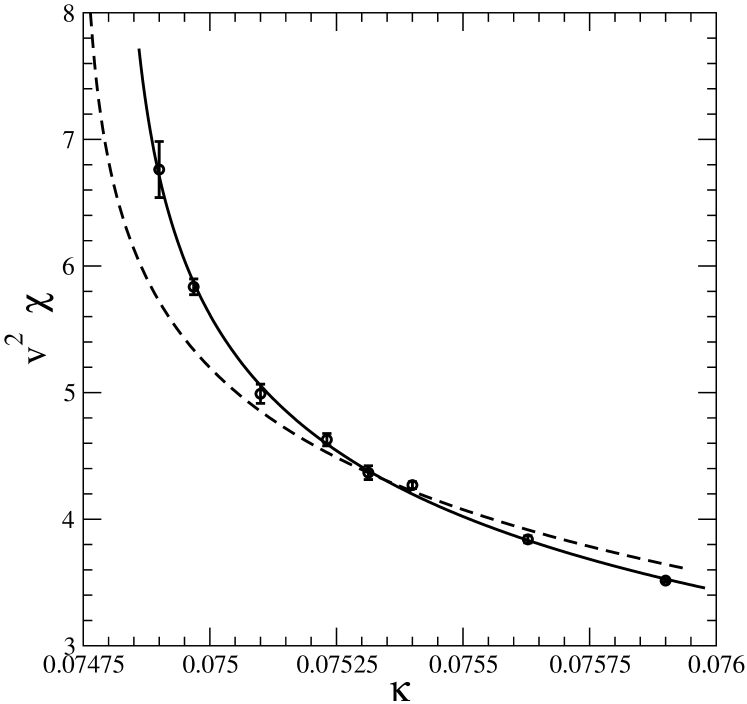
Figure 1: We show the lattice data for $v^{2}_{B}\chi_{\text{latt}}$ of Table 1 together with the fit Eq. (29) for $\gamma=2$ (solid line) and the two-loop fit Eq. (30) where the fit parameters are allowed to vary inside their theoretical uncertainties, $a_{1}=1.20(3)$ and $a_{2}=-1.6(5)$ (dashed line).

Nevertheless, one can adopt a pragmatic point of view, ignoring possible problems related to the matching conditions with the symmetric phase, and try to extract from the data for $v^{2}_{B}\chi_{2}(0)$ a new set of constants $C^{\prime}_{i}$. In particular the precise determination from $a_{1}=1.267(14)$ implies

$$C^{\prime}_{2}=6.67(4)$$ (33)

that will be used in the following.

Thus we can summarize the results of this section as follows:

1) leaving out the scale within the logs as a free parameter (and thus allowing effectively for the presence of next-to-leading corrections) the lattice data for $v^{2}_{B}\chi_{2}(0)$ are unable to distinguish between the powers $\gamma=1$ and $\gamma=2$. In this sense, a definitive test has to be postponed to simulations performed closer to the critical point where the non-leading terms associated with the scale of the logs should become unessential.

2) a 2-loop fit as in Eq.(30), with $a_{1}$ and $a_{2}$ deduced consistently from the LW tables, does not provide a good description of the data (see Fig.1). However, within the effective 2-loop formula Eq.(30), when $a_{1}$ and $a_{2}$ are left as free parameters, one can obtain precise determinations of the critical point $\kappa_{c}=0.074833(17)$ and of the integration constant $C^{\prime}_{2}=6.67(4)$. These will be used in the next section to check whether the lattice observables are consistent with the critical behaviour predicted by Renormalization Group (RG) analysis.

4 Lattice tests of the alternative interpretation of ‘triviality’. Part 2.

Additional numerical evidences concerning the relative scaling of $m_{H}$ and $\chi_{2}(0)$ can be obtained by comparing again with the predictions of perturbation theory. To this end, we performed in Ref.[1] a test of the logarithmic trend predicted in Eq.(9) assuming as input entries the full 3-loop values $m_{\text{input}}\equiv m_{R}$ reported in the first column of Table 3 of Ref. [18] at the various values of $\kappa$. These input mass values, to leading order, follow the scaling law

$$m_{H}=A\sqrt{\kappa-\kappa_{c}}\cdot|\ln(\kappa-\kappa_{c})|^{-1/6}$$ (34)

so that one can check whether the quantity

$$Z_{\varphi}\equiv 2\kappa m^{2}_{\text{input}}\chi_{\text{latt}}$$ (35)

tends to unity or grows logarithmically when approaching the continuum limit.

$m_{\text{input}}$	$\kappa$	lattice	algorithm	Ksweeps	$\chi_{\text{latt}}$	$v_{B}=\langle|\phi|\rangle$
0.4	0.0759	$32^{4}$	S-W	1750	41.714 (0.132)	0.290301 (21)
0.4	0.0759	$44^{4}$	W	60	41.948 (0.927)	0.290283 (52)
0.35	0.075628	$48^{4}$	W	130	58.699 (0.420)	0.255800 (18)
0.3	0.0754	$32^{4}$	S-W	345	87.449 (0.758)	0.220540 (75)
0.3	0.0754	$48^{4}$	W	406	87.821 (0.555)	0.220482 (19)
0.275	0.075313	$48^{4}$	W	53	104.156 (1.305)	0.204771 (40)
0.25	0.075231	$60^{4}$	W	42	130.798 (1.369)	0.188119 (31)
0.2	0.0751	$48^{4}$	W	27	203.828 (3.058)	0.156649 (103)
0.2	0.0751	$52^{4}$	W	48	201.191 (6.140)	0.156535 (65)
0.2	0.0751	$60^{4}$	W	7	202.398 (8.614)	0.156476 (148)
0.15	0.074968	$68^{4}$	W	25	460.199 (4.884)	0.112611 (51)
0.1	0.0749	$68^{4}$	W	24	1125.444 (36.365)	0.077358 (123)
0.1	0.0749	$72^{4}$	W	8	1140.880 (39.025)	0.077515 (210)

Table 1: The details of the lattice simulations for each $\kappa$ corresponding to $m_{\text{input}}$. In the algorithm column, ’S-W’ stands for the Swendsen-Wang algorithm [15], while ’W’ stands for the Wolff algorithm [16]. ’Ksweeps’ stands for sweeps multiplied by $10^{3}$.

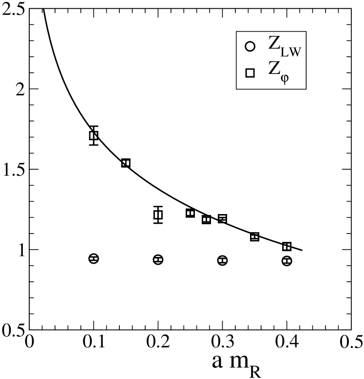
Figure 2: The lattice data for $Z_{\varphi}$, as defined in Eq. (35), and its perturbative prediction $Z_{\text{LW}}$ versus the input mass values $m_{\text{input}}=am_{R}$ taken from the LW Table. The solid line is a fit to the form $B\ln(\Lambda/m_{R})$ with $\Lambda=\pi/a$ and $B=0.50$.

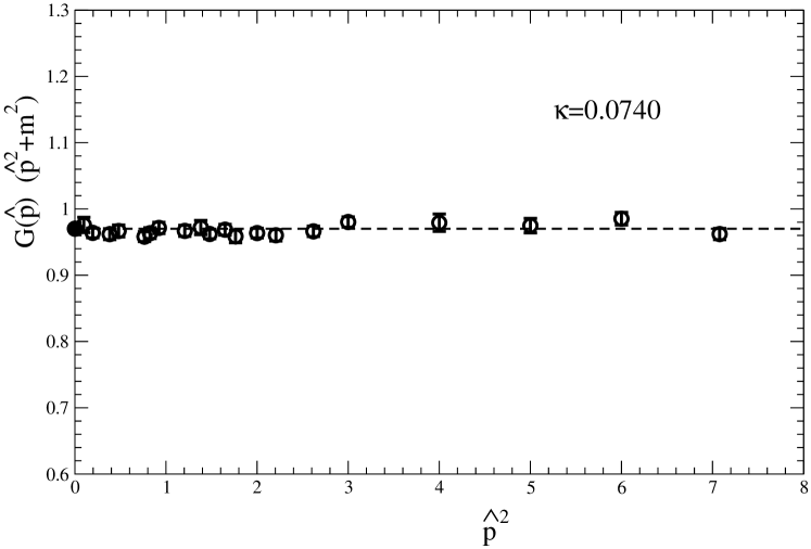
Figure 3: The lattice data for the re-scaled propagator in the symmetric phase at $\kappa=0.074$ as a function of the lattice momentum $\hat{p}_{\mu}=2\sin p_{\mu}/2$. The zero-momentum full point is defined as $Z_{\varphi}=(2\kappa)m^{2}_{\text{latt}}\chi_{\text{latt}}$. The dashed line indicates the value of $Z_{\text{prop}}$. Data are taken from Ref. [6].

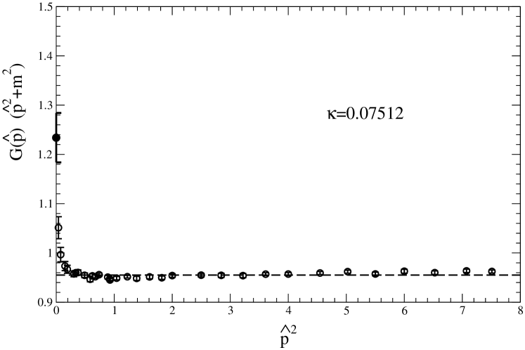
Figure 4: The lattice data for the re-scaled propagator in the broken phase at $\kappa=0.07512$ as a function of the lattice momentum $\hat{p}_{\mu}=2\sin p_{\mu}/2$. The zero-momentum full point is defined as $Z_{\varphi}=(2\kappa)m^{2}_{\text{latt}}\chi_{\text{latt}}$. The dashed line indicates the value of $Z_{\text{prop}}$. Data are taken from Ref. [6].

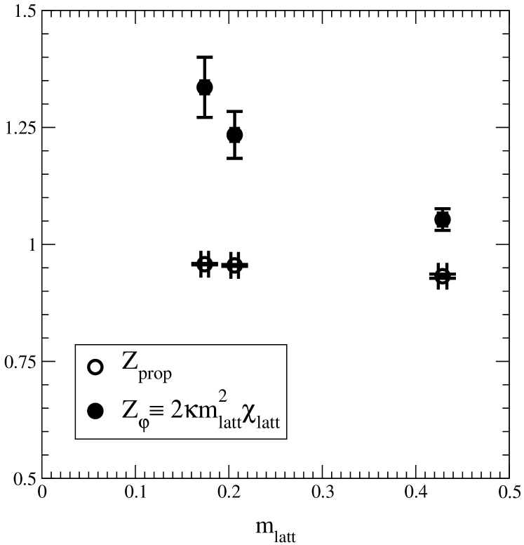
Figure 5: The two rescaling factors $Z_{\text{prop}}$ and $Z_{\phi}$ obtained in Ref. [6] as a function of $m_{\text{latt}}$.

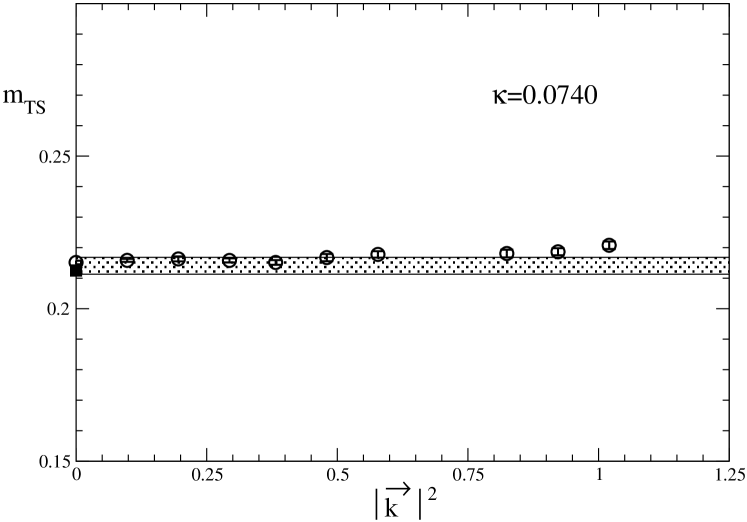
Figure 6: The time-slice mass $m_{\text{TS}}({\mathbf{k}})$ at different values of the three-momentum in the symmetric phase. The shaded area represents the value $m_{\text{latt}}=0.2141(28)$ obtained from the fit to the propagator data in Fig.3. The black square is the result of Ref. [19].

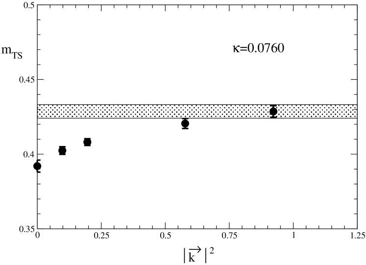
Figure 7: The time-slice mass $m_{\text{TS}}({\mathbf{k}})$ for several values of the spatial momentum in the broken phase. The zero-momentum value is our result $0.392(4)$ obtained from a simulation of 6 Msweeps on a $20^{4}$ lattice (in perfect agreement with the value $0.392(1)$ reported in Table 4 of Ref.[8]). The shaded area represents the value $m_{\text{latt}}=0.42865(456)$ obtained from the fit to the higher momentum propagator data.

Now, using in Eq.(35) the central values of $m_{\text{input}}\equiv m_{R}$ reported in the LW Table and the values of $\chi_{\text{latt}}$ reported in Table 1, the conclusion is unambiguous: the $Z_{\varphi}$ in Eq.(35) becomes larger and larger approaching the continuum limit along the RG curve $m_{\text{input}}=m_{\text{input}}(\kappa)$ and the observed increase is completely consistent with the logarithmic trend predicted in Eq.(9) (see Fig.2).

The discrepancy with the perturbative predictions can also be checked noticing that for $m_{\rm input}=0.08$ Ref. [18] predicts $\kappa=0.07481(8)$, i.e. smaller than $0.0749$. Therefore, by inspection of Table 1, the relevant lattice susceptibility will be definitely larger than its value for $\kappa=0.0749$, $\chi_{\rm latt}\sim 1100$, so that using Eq. (35), one gets the lower bound $Z_{\varphi}>1.05$ which cannot be reconciled with the perturbative predictions.

Balog et al. object to our conclusions that ”..the crucial question is whether the estimates $m_{\text{input}}$ of $m_{R}$ are reliable”. According to these authors, ”..the measured values of $m_{R}$ are considerably lower than the corresponding estimates $m_{\rm input}$” (i.e. the $m_{R}$’s that we took from the LW table). As a matter of fact, by replacing the LW $m_{R}$’s with the results of their simulations, one gets a remarkably constant value $2\kappa m^{2}_{R}\chi_{\text{latt}}\sim 0.88$.

Thus their objection does not concern our strategy but rather the validity of the LW entries themselves as reliable estimates of the Higgs mass parameter $m_{H}$. Actually, as we shall illustrate in the following, their conclusion does not apply: to check the true behaviour of $Z_{\varphi}=2\kappa m^{2}_{H}\chi_{\text{latt}}$ one should first identify correctly the operative definition of $m_{H}$ on the lattice. The mass values reported by Balog et al. are not reliable determinations of the physical Higgs mass if one requires the theoretical consistency of the adopted definition of ‘mass’. To fully appreciate what is going on, we need to go back to Refs. [5, 6, 7] (otherwise ignored by the authors of Ref.[8]).

In those calculations, one was fitting the lattice data for the connected propagator to the (lattice version of the) two-parameter form

$$G_{\text{fit}}(p)=\frac{Z_{\text{prop}}}{p^{2}+m^{2}_{\text{latt}}}\,.$$ (36)

This is a clean and simple strategy: there is no reason to restrict the analysis of the propagator to the limit $p\to 0$. In fact, in a free-field theory (the lattice version of) Eq.(36) is valid in the full range $0\leq p^{2}\leq\Lambda^{2}$ (with $\Lambda\sim\pi/a$). In a ‘trivial’ theory one expects a two-parameter fit to the propagator data to have small residual corrections. These, however, should become smaller and smaller by approaching the continuum limit.

In this way, after computing the lattice zero-momentum susceptibility $\chi_{\text{latt}}$, it becomes possible to compare the measured value of $Z_{\varphi}\equiv 2\kappa m^{2}_{\text{latt}}\chi_{\text{latt}}$ with the fitted $Z_{\text{prop}}$, both in the symmetric and broken phases. While no difference was found in the symmetric phase (see Fig. 3), $Z_{\varphi}$ and $Z_{\text{prop}}$ were found to be sizeably different in the broken phase. The discrepancy was found to become larger and larger by approaching the continuum limit and thus cannot be explained in terms of residual perturbative corrections to Eq.(36). In particular, $Z_{\text{prop}}$ was very slowly varying and steadily approaching unity from below in the continuum limit consistently with Kállen-Lehmann representation and ‘triviality’. $Z_{\varphi}$, on the other hand, was found to rapidly increase above unity in the same limit. The observed trend was consistent with the logarithmically increasing trend predicted in Eq.(9).

This conclusion was based on the values of $m_{\text{latt}}$ extracted by skipping the lowest 3-4 $p^{2}-$values in the fit to the propagator data. In fact, differently from the symmetric-phase simulations, where Eq.(36) reproduces the data in the full range $0\leq p^{2}\leq\Lambda^{2}$, in the broken-symmetry phase the two-parameter form Eq. (36) does not reproduce the propagator data down to $p=0$, see Fig.4 (and Figs.3,5,6 of Ref.[6]). Thus one has to choose. Either a) to restrict to the lowest 3-4 $p^{2}-$ data, and obtain from the fit a pair of values $(Z_{\text{low}},m_{\text{low}})$ or b) skip these first few data and fit the much larger sample of higher momentum data thus obtaining the other pair $(Z_{\text{high}},m_{\text{high}})$.

The two sets of mass values differ sizeably. For instance for $\kappa=0.076,0.07512,0.07504$ the results of Refs. [6] were respectively $m_{\text{high}}=0.4286(46),0.2062(41),0.1723(34)$. On the other hand, the alternative values from the lowest momentum data are respectively $m_{\text{low}}=0.392(4),0.1737(24),0.1419(17)$ for the same $\kappa$’s.

Numerically, the typical $m_{\text{low}}$’s are extremely close to the other mass definition $m_{\text{TS}}({\bf{k=0}})$, the mass extracted at zero 3-momentum from the exponential decay (TS=‘Time Slice’) of the connected two-point correlator

$$C_{1}(t,0;{\bf k})\equiv\langle S_{c}(t;{\bf k})S_{c}(0;{\bf k})+S_{s}(t;{\bf k})S_{s}(0;{\bf k})\rangle_{\rm conn},$$ (37)

where

$$S_{c}(t;{\bf k})\equiv\frac{1}{L^{3}}\sum_{{\bf x}}\phi({\bf x},t)\cos({\bf k}\cdot{\bf x}),$$ (38)

$$S_{s}(t;{\bf k})\equiv\frac{1}{L^{3}}\sum_{{\bf x}}\phi({\bf x},t)\sin({\bf k}\cdot{\bf x}).$$ (39)

Here, $t$ is the Euclidean time; ${\bf x}$ is the spatial part of the site 4-vector $x^{\mu}$; ${\bf k}$ is the lattice momentum ${\bf k}=(2\pi/L)(n_{x},n_{y},n_{z}$), with $(n_{x},n_{y},n_{z})$ non-negative integers; and $\langle...\rangle_{\rm conn}$ denotes the connected expectation value with respect to the lattice action, Eq. (22). In this way, parameterizing the correlator $C_{1}$ in terms of the energy $E_{k}$ as ($L_{t}$ being the lattice size in time direction)

$$C_{1}(t,0;{\bf k})=A\,[\,\exp(-E_{k}t)+\exp(-E_{k}(L_{t}-t))\,]\,,$$ (40)

the mass can be determined through the lattice dispersion relation

$$m^{2}_{\rm TS}({\bf k})=~{}2(\cosh E_{k}-1)~{}~{}-~{}~{}2\sum^{3}_{\mu=1}~{}(1-\cos k_{\mu})\,.$$ (41)

In a free-field theory $m_{\rm TS}$ is independent of k and coincides with $m_{\text{latt}}$ from Eq. (36).

Now, using the corresponding susceptibility values $\chi_{\text{latt}}=$37.85(6), 193.1(1.7), 293.4(2.9) reported in Ref. [6] and the above values of $m_{H}=m_{\text{high}}$ one obtains a set of logarithmically increasing values (see Fig.5): $Z_{\varphi}\equiv(2\kappa)m^{2}_{H}\chi_{\text{latt}}=1.05(2),1.23(5),1.31(5)$ as predicted in Refs.[2, 3, 4].

This is in contrast with the values of the other quantity $Z_{\text{low}}\sim\hat{Z}_{R}\equiv(2\kappa)m^{2}_{\text{low}}\chi_{\text{latt}}=0.884(18),0.875(24),0.887(21)$ which remain remarkably stable (see the corresponding entries for $\hat{Z}_{R}$ shown in Table 4 of Ref.[8]).

Therefore, the crucial question raised by the propagator data is the following. Which is the ‘true’ lattice definition of $m_{H}$ ? Is the $p\to 0$ choice (adopted by Balog et al.) and represented by $m_{\text{low}}\sim m_{\text{TS}}({\mathbf{k=0}})$, or that obtained from $m_{\text{high}}$, as proposed in Refs. [6]? As discussed in Ref.[6], there are several arguments that suggest the correct definition of $m_{H}$ to be obtained from $m_{\text{high}}$, thus regarding the other values extracted from the very low-momentum region as a symptom of the distinct dynamics of the scalar condensate. Here we list a few:

i) in the continuum theory, the shifted fluctuation field is defined as the $p_{\mu}\neq 0$ projection of the full quantum field. However in a lattice simulation with periodic boundary conditions, where the momenta $p_{i}$ are proportional to an integer number $n_{i}$ times the inverse lattice size $1/L$, the notion $p_{\mu}\neq 0$ is ambiguous. In fact, any finite set of integers will evolve onto the $p_{\mu}=0$ state in the limit $L\to\infty$. This means that, for a given lattice mass, by increasing the lattice size, to separate unambiguously the genuine finite-momentum fluctuation field from the ‘condensate’ itself, one should increase correspondingly the set of integers $n_{i}$. This gives a clean physical meaning to the fit obtained by skipping the lowest momentum propagator data and to the pair of parameters $(Z_{\text{high}},m_{\text{high}})$.

ii) the values obtained in Ref. [6] (respectively for $\kappa=$0.076, 0.07512,0.07504) $m_{\text{high}}=$0.4286(46), 0.2062(41), 0.1723(34) give a physical mass $m_{H}$ that scales as expected. This can easily be checked from the remarkable agreement between these values and the predicted trend Eq.(34) which is valid at the leading-log level both in perturbation theory and in the alternative picture of Refs.[2, 3, 4], see Eqs.(13) and (15). In this way one finds $A=17.282(364)$, $\kappa_{c}=0.074836(15)$ and predicts $m_{H}\sim$0.499, 0.408, 0.293, 0.199 for $\kappa=$0.0764, 0.0759, 0.0754, 0.0751 in good agreement with the values $0.5,0.4,0.3,0.2$ reported in the LW Table.

iii) the identification of $m_{\text{low}}\sim m_{\text{TS}}({\mathbf{k=0}})$ as the physical $m_{H}$ contradicts the observed dependence of $m_{\text{TS}}({\mathbf{k}})$ on $|{\mathbf{k}}|$ in the limit ${\mathbf{k}}\to 0$. In fact, in the symmetric phase (see Fig. 6) the energy spectrum has the form $\sqrt{{\mathbf{k}}^{2}+m^{2}}$ up to momenta ${\mathbf{k}}^{2}\sim 25m^{2}$(!). However in the broken phase the energy is not reproduced by the (lattice version of the) form $\sqrt{{\mathbf{k}}^{2}+{\text{const}}}$ (see Fig.7) and thus the very notion of ‘mass’ becomes problematic. At larger ${\mathbf{k}}$, where $m_{\text{TS}}({\mathbf{k}})$ becomes insensitive to ${\mathbf{k}}$, it agrees well with $m_{\text{high}}$. The very different behaviour between symmetric and broken phase shown in Figs. 6 and 7 has no counterpart in the conventional picture.

iv) the values of $Z_{\text{prop}}$ obtained from the fit to the higher-momentum data in Ref. [6] for $\kappa=0.076,0.07512,0.07504$, $Z_{\text{high}}=$0.9321(44), 0.9551(21), 0.9566(13), exhibit a monotonical increase toward unity (from below) as expected on the base of the Kállen-Lehmann representation in a ‘trivial’ theory. This confirms that fitting the propagator skipping the lowest momentum data gives consistent results. On the contrary, the values for $Z_{\text{low}}\sim\hat{Z}_{R}$ obtained from the fit to the lowest momentum points alone, remain constant to $\sim 0.88$ in the limit $\kappa\to\kappa_{c}$ (see also the values in Table 4 of Ref.[8]). Assuming this definition as the correct one to be used in the Källen-Lehmann representation, one would find an inner contradiction with the non-interacting nature of the shifted fluctuation field in the continuum limit.

No trace of this discussion is found in Ref.[8]. These authors, ignoring the evident difference between Fig.3 and Fig.4, as well as between Fig.6 and Fig.7, do not address the physical consistency of the mass definition extracted from the very low-momentum region of the lattice data. They just limit themselves to the remark that, for the $\lambda\Phi^{4}$ case, the lattice propagator is consistently reproduced by Eq.(36) for $p\to 0$. However, this agreement is not relevant here since the Ising limit is known to anticipate much better the true aspects of the theory in finite lattices. In the Ising case, in fact, the fit is not good and Balog et al. are forced to extract the lattice mass by fitting just to the three lowest momentum points, precisely as with the parameter $m_{\text{low}}$ of Ref. [6].

It is also surprising their claim (see the Abstract of Ref.[8]) that the lattice data are consistent with the perturbative predictions. We have seen in the previous section that, if one requires consistency between 2-loop predictions and the data for $v^{2}_{B}\chi_{2}(0)$, one has to replace the integration constant $C^{\prime}_{2}$ given in the LW’s Table 1 with the value $C^{\prime}_{2}=6.67(4)$ given in Eq.(33). Therefore, using the perturbative relation reported in Eq.(2.14) of Ref.[8], namely ($\alpha_{R}=\frac{g_{R}}{16\pi^{2}}$)

$$\hat{Z}_{R}=(2\kappa)C^{\prime}_{2}(1-\frac{7}{36}\alpha_{R}+{\cal O}(\alpha^{2}_{R}))$$ (42)

one can compare this $\hat{Z}_{R}$ with the other estimate extracted from the product $m^{2}_{R}\chi_{2}(0)$ and reported in Table 4 of Ref.[8].

In this case, for $\kappa=0.076$ (where the relevant value is $g_{R}=30.37(28)$) Eq.(42) predicts $\hat{Z}_{R}=0.976(6)$ while the value reported in Table 4 by Balog et al. is $\hat{Z}_{R}=0.896(4)$. Analogously, for $\kappa=0.0751$ (where the relevant values is $g_{R}=20.51(74)$) Eq.(42) predicts again $\hat{Z}_{R}=0.976(6)$ while the value reported in Table 4 by Balog et al. is $\hat{Z}_{R}=0.883(17)$. These discrepancies, that are at the level of $\sim 10\sigma$ and $\sim 5\sigma$, can hardly be considered indicative of theoretical consistency.

Quite independently, the authors of Ref.[8] have not shown that the $m_{R}$’s reported in their Table 4 lie on well defined RG trajectories $m_{R}=m_{R}(\kappa)$ using the same $\kappa_{c}=0.074833(17)$ obtained from the 2-loop fit to the data for $v^{2}_{B}\chi_{2}(0)$. In particular, this means that their value $m_{R}=0.395(1)$ for $\kappa=0.076$ has to come out consistent with the other value $m_{R}=0.1688(15)$ for $\kappa=0.0751$. To clarify this issue, they should quote the new values of the mass that replace the LW entries for all values of $\kappa$.

5 Summary and conclusions

Let us now try to summarize the various theoretical and numerical points addressed in this paper. We shall start by observing that the field rescaling is usually viewed as an ‘operatorial statement’ between bare and renormalized fields operators of the type

$$"~{}\Phi_{B}(x)=\sqrt{Z}\Phi_{R}(x)~{}"$$ (43)

As pointed out in Ref.[12], this relation is a consistent short-hand notation in a theory where the field operator admits an asymptotic Fock representation, as in QED. In the presence of spontaneous symmetry breaking it has no rigorous basis since the Fock representation exists only for the shifted fluctuating field $h_{B}(x)=\Phi_{B}(x)-\langle\Phi_{B}\rangle$, the one with a vanishing expectation value.

For this reason, following Refs.[2, 3, 4] (see the discussion given in Section 2), one can consider theoretical frameworks that are fully consistent with ‘triviality’ but where such an operatorial relation is not valid. In fact, the physical conditions used to determine the $h_{B}-h_{R}$ relation, through a $Z=Z_{\text{prop}}\sim 1$ in Eq.(4), can be basically different from those used in the $v_{B}-v_{R}$ case, through a $Z=Z_{\varphi}\sim\ln\Lambda$ in Eq.(6). In this case, if one wants to introduce a renormalized field operator $\Phi_{R}(x)$ (whose vacuum expectation value is what one defines by $v_{R}$ and whose fluctuating part is what one defines by $h_{R}$), this cannot be related to $\Phi_{B}(x)$ by means of Eq.(43).

As reviewed at the end of Section 2, this ‘subtlety’ has a substantial phenomenological implication: ‘triviality’, by itself, cannot be used to place upper bounds on the Higgs boson mass. Thus, the importance of the issue requires dedicated lattice simulations to check the validity of the logarithmic trend predicted in Eq.(9) by measuring the relative scaling of the physical Higgs mass squared $m^{2}_{H}$ vs. the zero-momentum susceptibility.

Clearly, the answer to this question depends on the given procedure adopted on the lattice to extract $m_{H}=m_{\text{latt}}$. Our point is that a correct choice requires to fulfill several consistency tests, taking into account the free-field nature of the fluctuation field in the continuum limit. Thus one should first find a 4-momentum region where the connected propagator is described by the (lattice version of the) two-parameter form

$$G_{\text{fit}}(p)=\frac{Z_{\text{prop}}}{p^{2}+m^{2}_{\text{latt}}}\,.$$ (44)

One should also check that the fitted value $m_{H}=m_{\text{latt}}$ controls the energy eigenvalues $E=E({\mathbf{k}})$ governing the exponential time decay of the connected correlator in a given region of 3-momentum ${\mathbf{k}}$. In fact, where the energy is not reproduced by the (lattice version of the) form $\sqrt{{\mathbf{k}}^{2}+{\text{const.}}}$, the very notion of mass becomes problematic. Finally, one should also check that the fitted values of $Z_{\text{prop}}$ approach unity from below in the continuum limit as required by the Kállen-Lehmann representation in a ‘trivial’ theory.

Now, the usual assumption is to extract $m_{H}=m_{\text{latt}}$ from the $p\to 0$ and/or ${\mathbf{k}}\to 0$ limits. This is certainly valid in a simulation performed in the symmetric phase (see Figs.3 and 6) where the whole 3- and 4-momentum regions give the same indications. However, in the broken-symmetry phase, where the vacuum is some sort of ‘condensate’, there might be reasons to avoid the strict zero-momentum limit to extract the physical particle mass.

For instance, as mentioned in Sect.4, in the continuum theory, the shifted fluctuation field is defined as the $p_{\mu}\neq 0$ projection of the full quantum field. However in a lattice simulation with periodic boundary conditions, where the momenta $p_{i}$ are proportional to an integer number $n_{i}$ times the inverse lattice size $1/L$, the notion $p_{\mu}\neq 0$ is ambiguous. In fact, any finite set of integers will evolve onto the $p_{\mu}=0$ state in the limit $L\to\infty$. Therefore, for a given lattice mass, by increasing the lattice size, to separate unambiguously the genuine finite-momentum fluctuation field from the ‘condensate’ itself, one should increase correspondingly the set of integers $n_{i}$.

In addition, there are precise physical motivations suggested by the non-relativistic limit of a broken-symmetry $\lambda\Phi^{4}$ theory: the low-temperature phase of a hard-sphere Bose gas [20]. In this case, the low-lying excitations for ${\mathbf{k}}\to 0$ are phonons, i.e. collective oscillations of the hard-sphere system whose energy grows linearly $E_{\text{ph}}({\mathbf{k}})\sim c_{s}|{\mathbf{k}}|$, $c_{s}$ being the speed of sound. Only at larger $|{\mathbf{k}}|$ does the energy spectrum grow quadratically. Therefore, a determination of the effective hard-sphere mass through the non-relativistic 1-particle relation $E_{\text{1-part}}({\mathbf{k}})\sim\frac{{\mathbf{k}}^{2}}{2m_{\text{eff}}}$ cannot be obtained from the ${\mathbf{k}}\to 0$ limit of the energy spectrum which is dominated by the phonon branch.

This type of problems were preliminarily considered in Ref. [6]. The result of that investigation was that the physical mass $m_{H}=m_{\text{latt}}$ is obtained from the propagator data after skipping the lowest 3-4 momentum points. The mass value $m_{\text{low}}$, obtained from the lowest momentum points, which is numerically close to the other mass extracted from the exponential decay of the connected correlator at zero 3-momentum, does not fulfill the same consistency checks.

Now, for $\kappa=0.076,0.07512,0.07504$ the results of Ref. [6] were respectively $m_{H}=m_{\text{latt}}=0.4286(46),0.2062(41),0.1723(34)$. In this way, using the susceptibility values $\chi_{\text{latt}}=$37.85(6), 193.1(1.7), 293.4(2.9) reported in Ref. [6] one obtains a set of logarithmically increasing values: $Z_{\varphi}\equiv(2\kappa)m^{2}_{H}\chi_{\text{latt}}=1.05(2),1.23(5),1.31(5)$ as predicted in Refs.[2, 3, 4] (see Fig.5). This is in contrast with the values obtained using $m_{\text{low}}$ for which the quantity $\hat{Z}_{R}\equiv(2\kappa)m^{2}_{\text{low}}\chi_{\text{latt}}\sim 0.88$ remains remarkably stable.

To provide further evidence, we replaced in Ref.[1] the direct evaluation of $m_{H}=m_{\text{latt}}$ with the theoretical input values predicted in the LW Tables. This is not in contradiction with the previous strategy, in fact the values obtained in Ref. [6] $m_{\text{latt}}=$0.4286(46), 0.2062(41), 0.1723(34) give a physical mass $m_{H}$ that scales as in Eq.(34) and that is in good agreement with the values $m_{H}=m_{\text{input}}(\kappa)$ reported in the LW Table. Using the values of $\chi_{\text{latt}}$ reported in our Table 1 and the LW entries for the mass, this additional test confirms that the quantity $Z_{\varphi}\equiv 2\kappa m^{2}_{\text{input}}\chi_{\text{latt}}$ increases logarithmically when approaching the continuum limit (see Fig.2).

Now, Balog et al., being aware that the above numerical evidences have ”..serious non standard implications for the Higgs sector of the Standard Model” (see the Conclusions of Ref.[8]), have performed a new analysis. They claim that the LW entries for $m_{R}$ should be replaced by new values (whose consistency with RG trajectories $m_{R}=m_{R}(\kappa)$, however, has not been shown). As far as we can see, they have essentially re-discovered the result of Ref. [6] that the quantity $\hat{Z}_{R}\equiv(2\kappa)m^{2}_{\text{low}}\chi_{\text{latt}}$ is a constant $\sim 0.88$. However, ignoring Ref. [6], they fail to appreciate why their values $m_{R}=m_{\text{low}}$ do not represent a consistent lattice definition of $m_{H}$.

A point where we accept their criticism concerns the lattice data for $v^{2}_{B}\chi_{2}(0)$. Restricting to this observable, a definitive test of the leading-logarithmic trend has to be postponed to data taken closer to the critical point where the non-leading terms associated with the scale of the logs should become unessential.

However, as discussed at the end of Sect.3, within the perturbative framework, the data for $v^{2}_{B}\chi_{2}(0)$ give precise information on the integration constants $C^{\prime}_{i}$ (i=1,2,3) that should be used for the matching with the symmetric phase. Using the precise outcome of the fit $C^{\prime}_{2}=6.67(4)$ Eq. (42) predicts $\hat{Z}_{R}\sim 0.976(6)$ with 5-10$\sigma$ discrepancies with respect to the values reported by Balog et al in their Table 4.

This is precisely the same discrepancy pointed out by Jansen et al. Ref.[21] whose origin cannot be understood ignoring the main point of Ref. [6] and of this paper. In the broken phase, a naive zero 4-momentum limit of the connected propagator and/or a naive zero 3-momentum limit of the energy eigenvalue controlling the exponential decay of the connected correlator, do not provide consistent estimates of the physical mass parameter $m_{H}$. The phenomenological implications are substantial. Once the quadratic shape of the effective potential (the inverse susceptibility), that is a pure zero-momentum quantity, does not scale uniformly with $m^{2}_{H}$, although the finite-momentum fluctuation field becomes free in the continuum limit, one cannot use ‘triviality’ to place upper bounds on $m_{H}$.

References

- [1] P. Cea, M. Consoli, and L. Cosmai, Large logarithmic rescaling of the scalar condensate: New lattice evidences, hep-lat/0407024.
- [2] M. Consoli and P. M. Stevenson, The non trivial effective potential of the ’trivial’ theory: a lattice test, Z. Phys. C63 (1994) 427–436, [http://arXiv.org/abs/hep-ph/9310338].
- [3] M. Consoli and P. M. Stevenson, Mode-dependent field renormalization and triviality in theory, Phys. Lett. B391 (1997) 144–149.
- [4] M. Consoli and P. M. Stevenson, Physical mechanisms generating spontaneous symmetry breaking and a hierarchy of scales, Int. J. Mod. Phys. A15 (2000) 133, [http://arXiv.org/abs/hep-ph/9905427].
- [5] P. Cea, M. Consoli, and L. Cosmai, First lattice evidence for a non-trivial renormalization of the Higgs condensate, Mod. Phys. Lett. A13 (1998) 2361–2368, [http://arXiv.org/abs/hep-lat/9805005].
- [6] P. Cea, M. Consoli, L. Cosmai, and P. M. Stevenson, Further lattice evidence for a large re-scaling of the Higgs condensate, Mod. Phys. Lett. A14 (1999) 1673–1688, [http://arXiv.org/abs/hep-lat/9902020].
- [7] P. Cea, M. Consoli, and L. Cosmai, Large rescaling of the Higgs condensate: Theoretical motivations and lattice results, Nucl. Phys. Proc. Suppl. 83 (2000) 658–660, [hep-lat/9909055].
- [8] J. Balog, A. Duncan, R. Willey, F. Niedermayer, and P. Weisz, The 4d one component lattice model in the broken phase revisited, hep-lat/0412015.
- [9] W. Zimmermann, Local Operator Products and Renormalization in Quantum Field Theory, vol. 1 of Brandeis University Summer Institute in Theoretical Physics 1970, p. 395. MIT Press, 1970.
- [10] V. Branchina, M. Consoli, and N. M. Stivala, Renormalization of massless lambda theories: Asymptotic freedom and spontaneous symmetry breaking, Z. Phys. C57 (1993) 251–266.
- [11] U. Ritschel, NonGaussian corrections to Higgs mass in autonomous in (3+1)-dimensions, Z. Phys. C63 (1994) 345–350, [hep-ph/9210206].
- [12] A. Agodi, G. Andronico, and M. Consoli, Lattice effective potential giving spontaneous symmetry breaking and the role of the Higgs mass, Z. Phys. C66 (1995) 439–452, [hep-lat/9410001].
- [13] P. M. Stevenson, B. Alles, and R. Tarrach, O(N) symmetric theory: the Gaussian effective potential approach, Phys. Rev. D35 (1987) 2407.
- [14] U. Ritschel, I. Stancu, and P. M. Stevenson, Unconventional large N limit of the Gaussian effective potential and the phase transition in theory, Z. Phys. C54 (1992) 627–634.
- [15] R. H. Swendsen and J.-S. Wang, Nonuniversal critical dynamics in Monte Carlo simulations, Phys. Rev. Lett. 58 (1987) 86–88.
- [16] U. Wolff, Collective Monte Carlo updating for spin systems, Phys. Rev. Lett. 62 (1989) 361.
- [17] D. S. Gaunt, M. F. Sykes, and S. McKenzie, Susceptibility and fourth-field derivative of the spin Ising model for and , J. Phys. A12 (1979) 871.
- [18] M. Lüscher and P. Weisz, Scaling laws and triviality bounds in the lattice theory. 2. One component model in the phase with spontaneous symmetry breaking, Nucl. Phys. B295 (1988) 65.
- [19] I. Montvay and P. Weisz, Numerical study of finite volume effects in the four- dimensional ising model, Nucl. Phys. B290 (1987) 327.
- [20] T. D. Lee, K. Huang, and C. N. Yang, Eigenvalues and Eigenfunctions of a Bose System of Hard Spheres and Its Low-Temperature Properties, Phys. Rev. 106 (1957) 1135–1145.
- [21] K. Jansen, T. Trappenberg, I. Montvay, G. Munster, and U. Wolff, Broken phase of the four-dimensional Ising model in a finite volume, Nucl. Phys. B322 (1989) 698.