Gluon field distribution in baryons

Abstract

Methods for revealing the distribution of gluon fields within the three-quark static-baryon potential are presented. In particular, we outline methods for studying the sensitivity of the source on the emerging vacuum response for the three-quark system. At the same time, we explore the possibility of revealing gluon-field distributions in three-quark systems in QCD without the use of gauge-dependent smoothing techniques. Renderings of flux tubes from a preliminary high-statistics study on a $12^{3}\times 24$ lattice are presented.

1 INTRODUCTION

Recently there has been renewed interest in studying the distribution of quark and gluon fields in the three-quark static-baryon potential. While early studies were inconclusive [1], improved computing resources and analysis techniques now make it possible to study this system in a quantitative manner [2, 3]. In particular, it is possible to directly compute the gluon flux distribution [4, 5] using lattice QCD techniques similar to those pioneered in mesonic static-quark systems [6, 7, 8].

Like Okiharu and Woloshyn [5] our first interest is to test the static-quark source-shape dependence of the observed flux distribution, as represented by correlations between the quark positions and the action or topological charge density of the gauge fields. To this end, we choose three different ways of connecting the gauge link paths required to create gauge-invariant Wilson loops. In the first case, quarks are connected along a T-shape path, while in the second case an L-shape is considered. Finally symmetric link paths approximating a Y-shape such that the quarks approximate an equilateral triangle are considered. The latter is particularly interesting as the probability of observing $\Delta$-shape flux-tubes are maximized in this equidistant case.

Because the signal decreases in an exponential fashion with the size of the loop, it is essential to use a method to enhance the signal. We use strict three-dimensional APE smearing [9] to enhance the overlap of our spatial-link paths with the ground-state static-quark baryon potential. Time-oriented links remain untouched to preserve the correct static quark potential at all separations.

Excellent signal to noise is achieved via a high-statistics approach based on translational symmetry of the four-dimensional lattice volume and rotational symmetries of the lattice as described in detail below. This approach contrasts previous investigations using gauge fixing followed by projection to smooth the links and resolve a signal in the flux distribution [4, 5].

2 WILSON LOOPS

To study the flux distribution in baryons on the lattice, one begins with the standard approach of connecting static quark propagators by spatial-link paths in a gauge invariant manner. APE-smeared spatial-link paths propagate the quarks from a common origin to their spatial positions.

The smearing procedure replaces a spatial link, $U_{\mu}(x)$, with a sum of $1-\alpha$ times the original link plus $\alpha/4$ times its four spatially oriented staples, followed by projection back to $SU(3)$. We select the unitary matrix $U_{\mu}^{\rm FL}$ which maximizes ${\cal R}e\,{\rm{tr}}(U_{\mu}^{\rm FL}\,U_{\mu}^{\prime\dagger})$, where $U_{\mu}^{\prime}$ is the smeared link, by iterating over the three diagonal $SU(2)$ subgroups of $SU(3)$ repeatedly. We repeat the combined procedure of smearing and projection $10$ times, with $\alpha=0.7$.

Untouched links in the time direction propagate the spatially separated quarks through Euclidean time. For sufficient time evolution the ground state is isolated. Finally smeared-link spatial paths propagate the quarks back to the common spatial origin.

The three-quark Wilson loop is defined as:

$$W_{3Q}=\frac{1}{3!}\epsilon^{abc}\epsilon^{a^{\prime}b^{\prime}c^{\prime}}\,U_{1}^{aa^{\prime}}\,U_{2}^{bb^{\prime}}\,U_{3}^{cc^{\prime}},$$ (1)

where $U_{j}$ is a staple made of path-ordered link variables

$$U_{j}\equiv P\exp\left(ig\int_{\Sigma_{j}}dx_{\mu}\,A^{\mu}(x)\right)\,,$$ (2)

and $\Sigma_{j}$ is the path along a given staple.

In this study, we consider two-dimensional spatial-link paths. Figures 1 and 2 give the projection of T and L shape paths in the $xy$ plane. Figure 3 shows the idea behind the Y-shape. In all cases the three quarks are created at the origin, O (white bubble), then are propagated to the positions Q1, Q2 or Q3 (black circle) before being propagated through time and finally back to a sink at the same spatial location as the source (O).

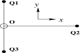
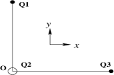
Figure 1: Projection of the T-shape path on the $xy$-plane.

Figure 2: Projection of the L-shape path on the $xy$-plane.

Figure 3: Projection of the Y-shape path on the $xy$-plane.

For the Y-shape we create elementary diagonal “links” in the form of boxes as shown in Fig. 4. The $1\times 1$ and $1\times 2$ boxes are the average of the two path-ordered link variables going from one corner to the diagonally opposite one. Taking both of these paths better maintains the symmetry of the ground state potential and therefore provides improved overlap with the ground state. We also consider $2\times 3$ boxes which are the averages of the possible paths connecting two opposite corners using 1x1 and 1x2 boxes. We will create further link paths in the future for use in bigger loops as necessary. Hence a diagonal staple is, in fact, an average of several “squared path” staples connecting the same end points.

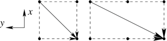
Figure 4: The diagonal path (solid line) is taken as the average of the two possible ones going around the box enclosing the end points.

The quark co-ordinates considered for Y-shape paths are summarized in Table 1. We note that the origin $(0,0)$ is not at the centre of these coordinates. Rather the coordinates are selected to place the quarks at approximately equal distances from each other.

$(x,y)$ Coordinates			Separation
$Q_{1}$	$Q_{2}$	$Q_{3}$	Cart.	Diagonal
$(0,1)$	$(1,-1)$	$(-1,-1)$	2	2.24
$(0,2)$	$(2,-1)$	$(-2,-1)$	4	3.61
$(0,3)$	$(2,-1)$	$(-2,-1)$	4	4.47
$(0,3)$	$(3,-2)$	$(-3,-2)$	6	5.83
$(0,4)$	$(4,-3)$	$(-4,-3)$	8	8.06
$(0,5)$	$(5,-4)$	$(-5,-4)$	10	10.3

Table 1: $(x,y)$ coordinates for the three quarks considered for Y-shape paths. The separation of the two quarks along a Cartesian (Cart.) direction are compared to the separation of those from the third quark.

3 GLUON FIELD CORRELATION

In this investigation we characterize the gluon field by the action density $S(\vec{y},t)$ observed at spatial coordinate $\vec{y}$ at Euclidean time $t$ measured relative to the origin of the three-quark Wilson loop. We calculate the action density using the highly-improved ${\cal O}(a^{4})$ three-loop improved lattice field-strength tensor [10] on four-sweep APE-smeared gauge links.

Defining the quark positions as $\vec{r}_{1}$, $\vec{r}_{2}$ and $\vec{r}_{3}$ relative to the origin of the three-quark Wilson loop, and denoting the Euclidean time extent of the loop by $T$, we evaluate the following correlation function

$$C(\vec{y};\vec{r}_{1},\vec{r}_{2},\vec{r}_{3};T)=$$ (3)

$$\quad\frac{\bigl{\langle}W_{3Q}(\vec{r}_{1},\vec{r}_{2},\vec{r}_{3};T)\,S(\vec{y},T/2)\bigr{\rangle}}{\bigl{\langle}W_{3Q}(\vec{r}_{1},\vec{r}_{2},\vec{r}_{3};T)\bigr{\rangle}\,\bigl{\langle}S(\vec{y},T/2)\bigr{\rangle}}\,,$$

where $\langle\cdots\rangle$ denotes averaging over configurations and lattice symmetries as described below. This formula correlates the quark positions via the three-quark Wilson loop with the gauge-field action in a gauge invariant manner. For fixed quark positions and Euclidean time, $C$ is a scalar field in three dimensions. For values of $\vec{y}$ well away from the quark positions $\vec{r}_{i}$, there are no correlations and $C\to 1$.

This measure has the advantage of being positive definite, eliminating any sign ambiguity on whether vacuum field fluctuations are enhanced or suppressed in the presence of static quarks. We find that $C$ is generally less than 1, signaling the expulsion of vacuum fluctuations from the interior of heavy-quark hadrons.

4 STATISTICS

For this work we consider 200 quenched QCD gauge-fields using the ${\cal O}(a^{2})$-mean-field improved Luscher-Weisz plaquette plus rectangle gauge action [11] on $12^{3}\times 24$ lattices at $\beta=4.60$, providing a lattice spacing of $a=0.123(2)$ fm as set by the string tension.

To improve the statistics of the simulation we use various symmetries of the lattice. First, we make use of translational invariance by computing the correlation on every node of the lattice, averaging the results over the four-volume.

To further improve the statistics, we use reflection symmetries. Through reflection on the plane $x=0$ we can double the number of T and Y-shaped Wilson loops. By using reflections on both the plane $x=0$ and $y=0$ we can quadruple the number of L-shaped loops.

We finally use $90^{\circ}$ rotational symmetry about the $x$-axis to double the number of Wilson loops. This means we are using both the $xy$ and $xz$ planes as the planes containing the quarks.

For this exploratory study we present images for $T=2$ and note that qualitatively similar results are observed for $T=4$. We plan to examine this and other similarly conservative alternatives on our anticipated larger lattice volumes providing further statistics improvement.

5 SIMULATION RESULTS

Figure 5 plots the correlation function of Eq. (3), $C(\vec{y})$, for an ortho-slice in the plane of the three-quark system. The colours of the ortho-slice, denoting the scalar values of $C(\vec{y})$, are rendered as a surface plot below. Away from the quark positions $C(\vec{y})\to 1$, but within the three-quark system $C(\vec{y})\sim 0.9$ indicating the suppression of QCD vacuum field fluctuations from the region inside heavy-quark hadrons. Here the quarks are approximately 0.75 fm from the centre of the distribution and are about 1.25 fm from each other.

Figure 6 renders the spatial points of $C(\vec{y})$ where the gluon action density is largely suppressed. Tube-like structures are revealed in Y-shape as opposed to $\Delta$ shape in accord with expectations from precision static quark-potential analyses.

We note that the centre of the flux tube is equidistant from the quark positions and not centered over the origin of the Wilson loop. This gives us confidence that sensitivity to the source is minimal. However it is important to examine this issue in greater detail and this will be the subject of a forthcoming publication.

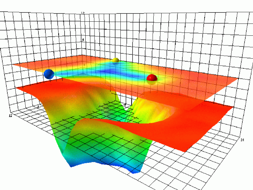
Figure 5: Ortho-slice and associated surface plot of the correlation function of Eq. (3), $C(\vec{y})$, observed for positions $\vec{y}$ in the plane of the three-quark system.

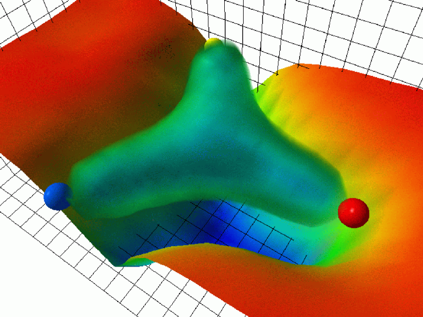
Figure 6: Spatial points where vacuum field fluctuations are maximally suppressed in the three-quark system as measured by the correlation function, $C(\vec{y})$, of Eq. (3). The surface plot is as in Fig. 5.

References

- [1] J. Flower, CALT-68-1378 (1986).
- [2] T. T. Takahashi, H. Suganuma, Y. Nemoto and H. Matsufuru, Phys. Rev. D65 (2002) 114509.
- [3] C. Alexandrou, Ph. de Forcrand and O. Jahn, Nucl. Phys. B (Proc. Suppl.) 119 (2003) 667.
- [4] H. Ichie, V. Bornyakov, T. Streuer and G. Schierholz, Nucl. Phys. B (Proc. Suppl.) 119 (2003) 751, hep-lat/0212036.
- [5] F. Okiharu and R. M. Woloshyn, Nucl. Phys. B (Proc. Suppl.) 129 (2004) 745, hep-lat/0310007.
- [6] R. Sommer, Nucl. Phys. B291 (1986) 673.
- [7] G. S. Bali, C. Schlichter and K. Schilling, Phys. Rev. D51 (1995) 5165.
- [8] R. W. Haymaker, V. Singh and Y. Peng, Phys. Rev. D53 (1996) 389.
- [9] M. Falcioni et al., Nucl. Phys. B251 (1985) 624; M. Albanese et al., Phys. Lett. B 192 (1987) 163.
- [10] S. O. Bilson-Thompson, D. B. Leinweber and A. G. Williams, Annals Phys. 304, 1 (2003) [hep-lat/0203008].
- [11] M. Luscher and P. Weisz, Commun. Math. Phys. 97, 59 (1985) [Erratum-ibid. 98, 433 (1985)].