Charmonium properties at finite temperature on quenched anisotropic lattices.

Abstract

We study charmonium properties below and above $T_{c}$ up to 1.8$T_{c}$, on quenched anisotropic lattices. Information of the spectral functions is extracted using the maximum entropy method and the constrained curve fitting. We also calculate the color singlet and averaged free energies and evaluate the charmonium spectrum with the potential model analysis. The relation between the lattice result of the spectral function analysis and the potential model is discussed.

1 Introduction

To investigate the properties of quark gluon plasma (QGP) in heavy ion collision experiments, theoretical prospects are significant, since such processes include complicated interactions among large number of particles. Changes of charmonium states have been regarded as one of the most important probes of plasma formation [1], because the potential model calculations predict the mass shift of charmonium near $T_{c}$ [2], and $J/\psi$ suppression above $T_{c}$ [3]. However, lattice QCD simulations have indicated that the thermal properties of hadronic correlators are much more involved than weakly interacting almost free quarks [4]. Recent studies of spectral functions of charmonium suggest that a hadronic excitation of $c$-$\bar{c}$ system may survives above $T_{c}$ [5, 6, 7]. This seems to conflict with the predictions of potential model approaches and a naive picture of QGP.

In this study we discuss the above disagreement between the spectral function analysis and the potential model. On one hand, we extract the information of the spectral function from the temporal charmonium correlator. On the other hand, we also extract the static quark potentials from the color singlet Polyakov loop correlation and Wilson loop. The result of potential model calculation using the latter is compared with the former.

These calculation are performed on quenched anisotropic lattices. This enables simulations at temperatures from $T\sim 0$ ($Nt=160$) to 1.75$T_{c}$ ($Nt=16$) keeping the lattice cutoff unique, to avoid uncertainties caused by the cutoff dependence in, for example, self-energy contribution to the potentials. The anisotropic lattice is also useful to keep the number of data points of the temporal correlators sufficiently large, which is important for detailed analysis of the spectral functions. We extend the simulation reported in Ref. [5] which was performed at the renormalized anisotropy $a_{\sigma}/a_{\tau}=4$, the spatial lattice cutoff is $a_{\sigma}^{-1}=2.0$GeV, and with the plaquette gauge and $O(a)$ improved Wilson quark actions. The critical temperature almost corresponds to $N_{t}=28$.

2 Spectral functions

To extract the spectral function from the temporal correlators, we adopt the maximum entropy method (MEM) and the constrained curve fitting (CCF) [8]. The result of the former provides the prior knowledge required for the latter. Combining the two methods, the results may be more reliable and quantitative than with one of them. In our previous study [5] we found that MEM fails to extract the spectral function from the correlator of local operators at $T>0$. Therefore we adopt spatially extended operators to enhance the low frequency mode of the spectral function. However the smeared operators may lead to an artificial peak, and thus careful analysis is necessary to distinguish the physical results from the artifact ones.

Although our MEM result shows that the spectral functions have peak structure in PS and V channels (corresponding to $\eta_{c}$ and $J/\psi$) at all temperature, the difference of result for different smearing functions, we call “smeared” and “half-smeared”, exists at higher temperature, especially above $1.4T_{c}$. This means that the peak structure of the spectral function at high temperature might be artificial. Furthermore we find large default model function dependence of the results, in which the position of the peak is stable but the peak width has large dependence. Therefore it is difficult to study the spectral function quantitatively using only MEM.

CCF analysis is performed based on the result of MEM, assuming the form of fitting function as the Breit-Wigner type,

$$A(\omega)=\sum_{i=1}^{N_{term}}\frac{\omega^{2}m_{i}\gamma_{i}R_{i}}{(\omega^{2}-m_{i}^{2})^{2}+m_{i}^{2}\gamma_{i}^{2}},$$ (1)

where $R_{i}$, $m_{i}$ and $\gamma_{i}$ are overlap, mass and width of the $i$-th peak respectively, and $N_{term}=2$ is used in this analysis. The result of lowest peak position (mass) and width are shown in Fig.1. Unfortunately, our results of the CCF is unstable against the prior knowledge as inputs. Therefore the systematic uncertainties will be larger than the quoted statistical error in Fig.1.

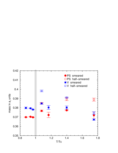
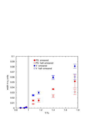
Figure 1: Temperature dependence of lowest peak mass, $m_{i}$, and width, $\gamma_{1}$, from the result of CCF analysis.

In spite of large systematic uncertainty, we can find the following tendency. Below $T_{c}$, the spectral function has a peak with almost the same mass at $T=0$ and vanishing width. Above $T_{c}$, the peak stays at similar position as at $T<0$ while its width tends to grow as temperature increases. As pointed out in the MEM analysis, however, the difference between the results of smeared and half-smeared correlators shows that a disappearance of the peak structure at higher $T$ cannot be excluded, especially in the V channel.

3 Static quark free energies

In this section we compare the results of spectral function with the potential model calculation. Here we define the following potentials.

$$V_{ave}(r) = -\ln{\langle\mbox{Tr}L(\vec{r})\mbox{Tr}L^{\dagger}(\vec{0})\rangle}/(N_{t}a_{\tau})$$ (2)

$$V_{sing}(r) = -\ln{\langle\mbox{Tr}L(\vec{r})L^{\dagger}(\vec{0})\rangle}/(N_{t}a_{\tau})$$ (3)

$$V_{Wilson}(r) \propto -\ln{W(\vec{r},t)}/t$$ (4)

where $L(\vec{r})$, $W(\vec{r},t)$ are Polyakov and Wilson loops, respectively. $V_{ave}$ is adopted in the former potential model calculations. $V_{sing}$ can not define in gauge independent form, then we calculate it in the Coulomb gauge, in which the $V_{sing}$ will be equivalent with a gauge invariant definition [9]. We can also define the other color singlet potential using the Wilson loops, $V_{wilson}$, which is calculated with the same way as at zero temperature. $V_{singlet}$ is thermal average of the energy spectrum of the color singlet $q-\bar{q}$ system, while $V_{wilsonloop}$ is the lowest one of the spectrum.

Figure 2 shows the result of $V_{sing},V_{Wilson}$ below and above $T_{c}$ respectively. Above $T_{c}$, unfortunately, we fail to extract the $V_{Wilson}$ and present only $V_{sing}$ in the bottom panel. We note that our results of $V_{ave}$ are consistent with previous studies, and draws the same conclusions as Refs. [2, 3].

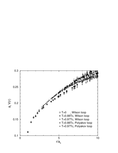
Figure 2: Color singlet static quark potentials ,$V_{sing}$ and $V_{Wilson}$, below and above $T_{c}$. $T=0$ result is also shown in both figures.

We solve the Schrödinger equation using the quark potential parametrized to the form, $V(r)=A_{1}+A_{2}/r+A_{3}\cdot r+A_{4}\cdot r^{2}$. Table 1 summarizes the result for the differences of binding energies from $T=0$. Below $T_{c}$, the CCF analysis found the mass difference of $-(0-10)$ MeV. Corresponding results of the potential model with $V_{sing}$ deviate from the CCF results, while those of $V_{Wilson}$ agree. Above $T_{c}$, $V_{sing}$ can hold a bound state up to $1.08T_{c}$, while at higher temperatures cannot, or at least the wave function become too broad compared to the spatial lattice size.

Table 1: Result of the Potential model analysis. The numbers mean difference from $T=0$ result.

$T/T_{c}(N_{t})$	$V_{sing}$ (MeV)	$V_{Wilson}$ (MeV)
$0.88(N_{t}=32)$	$+(71-87)$	$-(0-2)$
$0.97(N_{t}=29)$	$+(50-58)$	$-(21-23)$
$1.08(N_{t}=26)$	$-(170-180)$	none
$1.40(N_{t}=20)$	unbound	none

In summary, the disagreement between the results of spectral function analysis and the potential model is qualitatively absent if one uses the color singlet free energy as the static quark potential. This is the same conclusion as the Bielefeld group [10]. Detailed analysis of the quark potential indicated that the potential from the Wilson loop most well reproduces the result of spectral function analysis below $T_{c}$.

References

- [1] NA50 Collaboration, Phys. Lett. B 477 (2000) 28.
- [2] T. Hashimoto et al, Phys. Rev. Lett. 57 (1986) 2123.
- [3] T. Matsui and H. Satz, Phys. Lett. B 178 (1986) 416.
- [4] QCD-TARO Collaboration, Phys. Rev. D 63 (2001) 054501; T. Umeda et al., Int. J. Mod. Phys. A 16 (2001) 2215.
- [5] T. Umeda, et al., Eur. Phys. J. C (2004), DOI 10.1140/epjcd/s2004-01-002-1 (hep-lat/0211003).
- [6] S. Datta et al., J. Phys. G30 (2004) S1347.
- [7] M. Asakawa and T. Hatsuda, Phys. Rev. Lett. 92 (2004) 012001.
- [8] G. P. Lepage et al., Nucl. Phys. B(Proc.Suppl.) 106 (2002) 12.
- [9] O. Philipsen, Phys. Lett. B535 (2002) 138.
- [10] F. Karsch, J. Phys. G 30 (2004) S887.