Genuine Symmetry of Staggered Fermion

Abstract:

We present a new formulation of the staggered fermion on the $D$-dimensional lattice based on the $SO(2D)$ Clifford algebra, which is naturally present in the action. The action of the massless staggered fermion is invariant under the discrete rotation and the $SO(2D)$ chiral and other discrete transformations. From transformation properties of the fermion, we find two local meson operators (one scalar and one pseudoscalar) in addition to two standard meson operators.

1 Introduction

The fermions on lattice are bound to suffer from the doubling problem. In the early stage of the development of the lattice gauge theory, it is proposed that massless modes due to the doubling may be regarded as internal (flavor) degrees of freedom [1, 2]. The naively discretized Dirac fermion was formulated as a staggered fermion in Ref. [3]. The reconstruction procedure was found to give spinors with flavor degrees of freedom for the staggered fermion with one component spinor on each site [4].

Since the spinor and flavor degrees of freedom originate from its geometrical structure, the staggered fermion must transform nontrivially under the rotation. To clarify it is one of the main motivations of the present paper. In this paper, we consider the one component staggered fermion in $D$ dimensions, which has $2^{D}$ degrees of freedom due to the doubling. The number coincides with the dimension of the spinor representation of $SO(2D)$. Indeed, we will show that the $SO(2D)$ Clifford algebra is naturally present in the theory and it plays a crucial role to study symmetries of the staggered Dirac operator. We study the (discrete) rotational symmetry, the chiral symmetry and other discrete transformations such as parity, charge conjugation and time reversal.

Symmetries of the staggered fermion have been discussed earlier in Ref.[5]. Our approach differs from theirs on two important points: 1) The $SO(2D)$ structure is fully respected ; 2) We use a different definition for the rotation, which, we believe, is more suitable for the staggered fermion. The details will be discussed in section 3.

With the knowledge of symmetries, we find two extra meson operators, more than those well-known scalar and pseudoscalar operators. These operators have been overlooked in simulations and it is very important to take them into account for a reliable study.

2 The Staggered Fermion and $SO(2D)$ Clifford Algebra

In this section, we present a new expression of the staggered Dirac operator based on the $SO(2D)$ Clifford algebra to be found for the $D$-dimensional lattice. For the purpose, it is important to understand the geometrical structure associated with the staggered fermion and its relation to the $SO(2D)$ Clifford algebra. This will be explained in the next subsection. Then we proceed to the expression of the staggered Dirac operator that respects the algebra.

2.1 Geometrical structure of the staggered fermion

To clearly state the geometrical structure, we classify links, plaquettes and hypercubes.

Consider the link directed to the positive $\mu$ direction from the site $n_{\mu}$. We denote it by $(n,\mu)$ and assign the sign factor, $(-1)^{n_{\mu}}$. As for the link directed to the negative direction, we write it as $(n,-\mu)$ and the associated sign factor must be $(-1)^{n_{\mu}+1}$. The plaquette $(n,\mu\nu)$ is defined as the ordered links,

$$(n,\mu\nu)\equiv(n,\mu)(n+\hat{\mu},\nu)(n+\hat{\mu}+\hat{\nu},-\mu)(n+\hat{\nu},-\nu)~{}~{}~{}~{}~{}(\mu<\nu).$$ (1)

On each link of $(n,\mu\nu)$, we have a sign factor. We refer to the plaquette with $(++++)$ or $(----)$ sign factors as a cell-plaquette, while that with a set of mixed signs as a pipe-plaquette. On any two dimensional surface of the $D$-dimensional lattice, we find the checkered pattern, or the Ichimatsu pattern, formed by the cell- and pipe-plaquettes.

Note that there are distinctive hypercubes on the lattice: Those formed solely by cell-plaquettes with all plus (minus) sign factors will be called microcells (macrocells) by the reason to be explained shortly. The coordinates $(n_{\mu})$ of sites on a microcell can be written as $n_{\mu}=2N_{\mu}+r_{\mu}$, where $N_{\mu}$ is some integer and $r_{\mu}$ takes the value of $0$ or $1$. As for a macrocell, those are written similarly as $n_{\mu}=2N_{\mu}+1+r_{\mu}$.

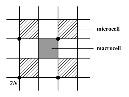
Figure 1: The microcells and macrocells

After having introduced the notions of micro- and macrocells, we observe a slightly more detailed structure on a two dimensional surface than the Ichimatsu pattern. The $D=2$ example is shown in Fig.1, where a microcell (macrocell) is shown as a shaded (gray) square. We would find the same pattern on any two dimensional surface of the $D$-dimensional lattice. It is noteworthy to realize that the pattern is invariant under the translation by twice the lattice spacing, $2a$. We call this translation the modulo 2 translation.

After the reconstruction, the Grassmann variables on the sites of a microcell are to form a spinor labelled by $(N_{\mu})$. The relative coordinates $(r_{\mu})$ on the Grassmann variables are transformed into spinor and flavor indices. In this sense, a microcell may be regarded as an internal space. The global structure such as the fermion kinetic term are formed out of the remaining geometrical structure.

The relation of the staggered fermion to the $SO(2D)$ Clifford algebra comes from the fact that sites on a microcell can be regarded as the weight lattice for the spinor representation of $SO(2D)$. Therefore the Grassmann variables on sites in a microcell are in the spinor representation. Accordingly, we will find that the Dirac operator has a natural expression in terms of gamma matrices associated with this $SO(2D)$.

In the next section, we will consider the symmetry of the action under the $\pi/2$ rotation around the center of a microcell. One could have considered the $\pi/2$ rotation around a site. Actually, the latter rotation was studied earlier in Ref. [5] and the rotational symmetry of the staggered fermion was established. These two rotations are to end up with the same rotational symmetry in the continuum limit. We choose the former definition to respect the geometrical structure explained above that is inherent to the staggered fermion.

2.2 The staggered Dirac operator

The single component staggered Dirac operator is given as

$$(D_{\rm st})_{n,n^{\prime}} = \sum_{\mu}\eta_{\mu}(n)\frac{\delta_{n^{\prime},n+\hat{\mu}}U^{\rm rep}_{n,\mu}-\delta_{n^{\prime},n-\hat{\mu}}U^{{\rm rep}\hskip 1.42262pt\dagger}_{n-\hat{\mu},\mu}}{2a},$$ (2)

where $\eta_{\mu}(n)=\eta_{\mu}(r)=(-1)^{\sum_{\nu<\mu}r_{\nu}}$. The link variable $U^{\rm rep}_{n,\mu}$ acts on the fermion variable in the representation “rep” of the gauge group. For simplicity, we drop the superscript “rep” from the link variable in the rest of the paper.

In preparation to rewrite the operator in eq. (2) to act on the coordinates $(r,N)$, we introduce notations for gamma matrices and their products for the $SO(2D)$ Clifford algebra. By $\vec{\varepsilon}$, we denote a bit-valued $D$-dimensional vector: That is, each entry takes the value of $0$ or $1$. For each $\vec{\varepsilon}$, we define the matrix

$$(\Gamma_{\mu,\vec{\varepsilon}})_{(r_{1},r^{\prime}_{1})\cdots(r_{D},r^{\prime}_{D})} \equiv \Bigl{(}(\sigma_{3}{}^{\varepsilon_{1}}\otimes\cdots\otimes\sigma_{3}{}^{\varepsilon_{D}})$$

$$\times(\sigma_{3}\otimes\cdots\otimes\sigma_{3}\otimes\stackrel{{\scriptstyle\raise 5.0pt\hbox{\scriptsize$\mu$}\mbox{ }}}{{\sigma_{1}}}\otimes{\bf 1}\otimes\cdots\otimes{\bf 1})\Bigr{)}_{(r_{1},r^{\prime}_{1})\cdots(r_{D},r^{\prime}_{D})}.$$

As special cases, we obtain a basis for the $SO(2D)$ Clifford algebra,

$$\gamma_{\mu}=\Gamma_{\mu,\vec{0}},~{}~{}~{}~{}~{}\tilde{\gamma}_{\mu}=-i\Gamma_{\mu,\vec{e}_{\mu}},$$ (4)

with $\vec{e}_{\mu}$ being the unit vector along the $\mu$-direction. Note that $\gamma_{\mu}$ in eq. (4) are for an irreducible representation of the $SO(2D)$ Clifford algebra while they are reducible as for the $SO(D)$ Clifford algebra. In terms of the basis given in eq. (4), eq. (2.2) may be expressed as

$$(\Gamma_{\mu,\vec{\varepsilon}})_{(r_{1},r^{\prime}_{1})\cdots(r_{D},r^{\prime}_{D})}=\Bigl{(}(i\tilde{\gamma}_{1}{\gamma_{1}})^{\varepsilon_{1}}\cdots(i\tilde{\gamma}_{D}{\gamma_{D}})^{\varepsilon_{D}}\gamma_{\mu}\Bigr{)}_{(r_{1},r^{\prime}_{1})\cdots(r_{D},r^{\prime}_{D})}.$$ (5)

We may rewrite $(D_{\rm st})_{n,n^{\prime}}$ as an operator acting on the coordinates $(r,N)$. That is realized by using the expression (2.2),

$$(D_{\rm st})_{n,n^{\prime}}\equiv(D_{\rm st})_{(r,N),(r^{\prime},N^{\prime})} = \sum_{\mu,\vec{\varepsilon}}(\Gamma_{\mu,\vec{\varepsilon}})_{(r,r^{\prime})}(D_{\mu,\vec{\varepsilon}})_{(N,N^{\prime})}.$$ (6)

Here $D_{\mu,\vec{\varepsilon}}$ is the generalized difference operator,

$$(D_{\mu,\vec{\varepsilon}})_{(N,N^{\prime})} = {1\over 2^{D}}\sum_{\vec{\sigma}}(-1)^{\vec{\varepsilon}\cdot\vec{\sigma}}(\nabla_{\mu}^{\vec{\sigma}})_{(N,N^{\prime})},$$ (7)

with

$$(\nabla_{\mu}^{\vec{\sigma}})_{(N,N^{\prime})} = \left\{\begin{array}[]{l}{1\over 2a}\left(\delta_{N,N^{\prime}}U_{2N+\vec{\sigma},\mu}-\delta_{N-\hat{\mu},N^{\prime}}U^{{\dagger}}_{2N+\vec{\sigma}-\hat{\mu},\mu}\right),\qquad\sigma_{\mu}=0,\\[18.0pt] {1\over 2a}\left(\delta_{N+\hat{\mu},N^{\prime}}U_{2N+\vec{\sigma},\mu}-\delta_{N,N^{\prime}}U^{{\dagger}}_{2N+\vec{\sigma}-\hat{\mu},\mu}\right),\qquad\sigma_{\mu}=1.\end{array}\right.$$ (10)

Note that $\sigma_{\mu}=0$ and $1$ give the backward and forward difference operators respectively. As observed in eq. (7), the $D$-dimensional bit-valued vector $\vec{\sigma}$ is dual to $\vec{\varepsilon}$.

In the last expression of eq. (6), the Dirac operator is decomposed into the difference operator acting on the microcell coordinate $(N_{\mu})$ and the matrix acting on the relative coordinate $(r_{\mu})$. Accordingly, we collectively treat the fermion variables on sites in a microcell by introducing the new variables:

$$\Psi_{r}(N)\equiv\xi_{2N+r},~{}~{}~{}{\bar{\Psi}}_{r}(N)\equiv{\bar{\xi}}_{2N+r}.$$ (11)

The new fermion variables $\Psi_{r}(N)$ and ${\bar{\Psi}}_{r}(N)$ belong to spinor representations of $SO(2D)$.

3 Symmetries of Staggered Fermion

The single component staggered fermion action is invariant under the discrete rotation, the chiral transformation, parity and charge conjugation. Here we explain these symmetries. In particular, we will find that the $SO(2D)$ Clifford algebra plays a vital role to describe the rotational discrete symmetry. Also, the well-known chiral transformation will be identified with the $U(1)_{A}$ chiral transformation associated with the $SO(2D)$ Clifford algebra.

3.1 Rotation

Let us see how the coordinates are transformed under the $\pi/2$ rotation around the center of the microcell. Without losing the generality, we may take the microcell attached to the origin and rotate the system around the center of the microcell. We consider the $\mu(<)\nu$ rotation. It is easy to find out the following transformation rules: For the relative coordinates,

$$(r_{R})_{\rho}=\left\{\begin{array}[]{ll}r_{\rho},&\rho\neq\mu,\nu,\\ 1-r_{\nu},&\rho=\mu,\\ r_{\mu},&\rho=\nu;\end{array}\right.$$ (15)

and for the coordinate $N_{\rho}$,

$$(N_{R})_{\rho}=\left\{\begin{array}[]{ll}N_{\rho},&\rho\neq\mu,\nu,\\ -N_{\nu},&\rho=\mu,\\ N_{\mu},&\rho=\nu.\end{array}\right.$$ (19)

Here the subscript $R$ implies rotated quantities. For the simplicity of the notation, we do not write the subscripts $\mu\nu$ explicitly.

The transformation of the generalized difference operator is found to be

$$D^{R}_{\rho,\vec{\varepsilon}}(N,N^{\prime})=\left\{\begin{array}[]{ll}(-1)^{\varepsilon_{\mu}}D_{\rho,\vec{\varepsilon}_{R}}(N_{R},N^{\prime}_{R}),&\rho\neq\mu,\nu,\\ (-1)^{\varepsilon_{\mu}+1}D_{\nu,\vec{\varepsilon}_{R}}(N_{R},N^{\prime}_{R}),&\rho=\mu,\\ (-1)^{\varepsilon_{\mu}}D_{\mu,\vec{\varepsilon}_{R}}(N_{R},N^{\prime}_{R}),&\rho=\nu,\end{array}\right.$$ (23)

where

$$(\varepsilon_{R})_{\rho}=\left\{\begin{array}[]{ll}\varepsilon_{\rho},&\rho\neq\mu,\nu,\\ \varepsilon_{\nu},&\rho=\mu,\\ \varepsilon_{\mu},&\rho=\nu.\end{array}\right.$$ (27)

The staggered Dirac operator consists of two factors, $D_{\rho,\vec{\varepsilon}}$ and $\Gamma_{\rho,\vec{\varepsilon}}$. Having obtained the transformation property of the former, we need to find the transformation of the latter that compensates the sign factors in eq. (23) so that the Dirac operator transforms as

$$D_{\rm st}^{R}=V_{\mu\nu}D_{\rm st}V_{\mu\nu}^{\dagger}$$ (28)

with a matrix $V_{\mu\nu}$. When this is realized, the transformations of $\Psi$ and ${\bar{\Psi}}$ are to be

$$\Psi_{R}(N) = V_{\mu\nu}\Psi(N_{R}),$$

$${\bar{\Psi}}_{R}(N) = \bar{\Psi}(N_{R})V_{\mu\nu}^{\dagger},$$ (29)

in order for the single staggered fermion action,

$$S=\sum{\bar{\Psi}}D_{st}\Psi,$$ (30)

to be invariant.

In order to realize (28), we require that $\Gamma_{\rho,\vec{\varepsilon}}$ transform as

$$V_{\mu\nu}\Gamma_{\rho,\vec{\varepsilon}}V_{\mu\nu}^{\dagger}=\left\{\begin{array}[]{ll}(-1)^{\varepsilon_{\mu}}\Gamma_{\rho,\vec{\varepsilon}_{R}},&\rho\neq\mu,\nu,\\ (-1)^{\varepsilon_{\mu}+1}\Gamma_{\nu,\vec{\varepsilon}_{R}},&\rho=\mu,\\ (-1)^{\varepsilon_{\mu}}\Gamma_{\mu,\vec{\varepsilon}_{R}},&\rho=\nu.\end{array}\right.$$ (34)

The matrix $V_{\mu\nu}$ is to found from this condition (34). After some efforts, we find the matrix of desired property,

$$V_{\mu\nu}=\frac{1}{2}\Gamma_{2D+1}(\tilde{\gamma}_{\mu}-\tilde{\gamma}_{\nu})(1+\gamma_{\mu}\gamma_{\nu}).$$ (35)

Note that the condition (34) determines the matrix $V_{\mu\nu}$ up to a phase factor.

By combining eqs. (23) and (34), we easily see that the Dirac operator transforms as eq. (28) . Therefore, we conclude that the single staggered fermion action is invariant under the discrete rotational transformation.

From eq. (34), it is easy to find the action of $V_{\mu\nu}$ on the basis of the $SO(2D)$ Clifford algebra:

$$V_{\mu\nu}\gamma_{\rho}V_{\mu\nu}^{\dagger}=\left\{\begin{array}[]{ll}\gamma_{\rho},&\rho\neq\mu,\nu,\\ -\gamma_{\nu},&\rho=\mu,\\ \gamma_{\mu},&\rho=\nu,\end{array}\right.\qquad V_{\mu\nu}\tilde{\gamma}_{\rho}V_{\mu\nu}^{\dagger}=\left\{\begin{array}[]{ll}\tilde{\gamma}_{\rho},&\rho\neq\mu,\nu,\\ \tilde{\gamma}_{\nu},&\rho=\mu,\\ \tilde{\gamma}_{\mu},&\rho=\nu.\end{array}\right.$$ (42)

Here, note that ${\tilde{\gamma}}_{\mu}$ do not transform as a vector: The action of $V_{\mu\nu}$ simply exchanges ${\tilde{\gamma}}_{\mu}$ for ${\tilde{\gamma}}_{\nu}$.

Related to the transformation in eq. (42), there is a further curious feature of the matrix $V_{\mu\nu}$. We studied the $\pi/2$ rotation around the center of a microcell which leaves the system invariant. This intuitively obvious rotation causes a quite nontrivial transformation among sites in a microcell, or the weight lattice of the $SO(2D)$ spinor representation. We found that this was achieved by the matrix $V_{\mu\nu}$. In eq. (42), note that negative is the determinant of the transformation matrix realized on the matrices $\gamma_{\mu}$ and ${\tilde{\gamma}}_{\mu}$. Therefore the transformation generated on the $2D$ gamma matrices belongs to $O(2D)$ but not to $SO(2D)$. In the continuum limit, the staggered Dirac operator becomes flavor blind. As a result, the transformation in eq. (28) reduces to the $\pi/2$ rotation in the $D$-dimensional space.

3.2 Chiral symmetry

It is known that the staggered fermion action is invariant under the transformation

$$\xi_{n}^{\prime}=(-1)^{|n|}\xi_{n},~{}~{}~{}~{}~{}{\bar{\xi}}_{n}^{\prime}=(-1)^{|n|+1}{\bar{\xi}}_{n}.$$ (43)

This symmetry forbids the fermion mass term, even for odd dimensions. In this sense, the symmetry has been regarded as a sort of chiral symmetry for the staggered fermion, though the origin of the symmetry has not been clearly understood. Here we show that this symmetry is nothing but the $U(1)_{A}$ chiral transformation associated with the $SO(2D)$ Clifford algebra,

$$\Psi^{\prime}=\exp(i\theta\Gamma_{2D+1})\Psi,~{}~{}\bar{\Psi}^{\prime}=\bar{\Psi}\exp(i\theta\Gamma_{2D+1}),$$ (44)

with

$$\Gamma_{2D+1}(r,r^{\prime}) = (-i)^{D}(-1)^{\frac{D(D-1)}{2}}(\gamma_{1}\cdots\gamma_{D}\tilde{\gamma}_{1}\cdots\tilde{\gamma}_{D})(r,r^{\prime})$$ (45)

$$= (\sigma_{3}\otimes\cdots\otimes\sigma_{3})(r,r^{\prime})=(-1)^{|r|}\delta_{r,r^{\prime}}.$$

Taking $\theta=\pi/2$ in eq.(44), we have $\Psi_{r}^{\prime}(N)=i(-1)^{|r|}\Psi_{r}(N)$ and ${\bar{\Psi}}_{r}^{\prime}(N)=i(-1)^{|r|}{\bar{\Psi}}_{r}(N)$, that can be rewritten as eq. (43) for $\xi$ and $\bar{\xi}$ variables.

By using the properties,

$$\{\Gamma_{2D+1},\gamma_{\mu}\}=\{\Gamma_{2D+1},\tilde{\gamma}_{\mu}\}=\{\Gamma_{2D+1},\Gamma_{\mu,\vec{\varepsilon}}\}=0,$$ (46)

we obtain the relation

$$\exp{(i\theta\Gamma_{2D+1})}D_{\rm st}\exp{(i\theta\Gamma_{2D+1})}=D_{\rm st}.$$ (47)

Therefore, the action (30) is invariant under the chiral transformation in any even as well as odd dimensions.

In the rest of this section, we describe discrete symmetries starting with the parity symmetry.

3.3 Parity and charge conjugation

We take the reflection as the definition of the parity. The reflection along $\mu$ direction, $P_{\mu}$, only affects the $\mu$-components of coordinates,

$$[N_{\mu}]_{P_{\mu}}=-N_{\mu},~{}~{}~{}~{}~{}[\sigma_{\mu}]_{P_{\mu}}=1-\sigma_{\mu},$$

and a link variable transforms as,

$$[U_{2N+\vec{\sigma},\rho}]_{P_{\mu}}=\left\{\begin{array}[]{ll}U_{[2N+\vec{\sigma}]_{P_{\mu}},\rho},&\rho\neq\mu,\\ U^{\dagger}_{[2N+\vec{\sigma}]_{P_{\mu}},\rho},&\rho=\mu.\end{array}\right.$$

Therefore, we find

$$[D_{\rho,\vec{\varepsilon}}]_{P_{\mu}}=\left\{\begin{array}[]{ll}(-1)^{\varepsilon_{\mu}}D_{\rho,\vec{\varepsilon}},&\rho\neq\mu,\\ (-1)^{\varepsilon_{\mu}+1}D_{\mu,\vec{\varepsilon}},&\rho=\mu.\end{array}\right.$$ (51)

The matrix $V_{\mu}\equiv\Gamma_{2D+1}{\gamma}_{\mu}$ produces the appropriate sign factors by acting on $\Gamma_{\rho,\varepsilon}$:

$$V_{\mu}\Gamma_{\rho,\vec{\varepsilon}}V^{\dagger}_{\mu}=\left\{\begin{array}[]{ll}(-1)^{\varepsilon_{\mu}}\Gamma_{\rho,\vec{\varepsilon}},&\rho\neq\mu,\\ (-1)^{\varepsilon_{\mu}+1}\Gamma_{\mu,\vec{\varepsilon}},&\rho=\mu~{}.\end{array}\right.$$ (54)

From eqs. (51) and (54), we find the Dirac operator transforms as $[D_{\rm st}]_{P_{\mu}}=V_{\mu}D_{\rm st}V_{\mu}^{\dagger}$. This implies the action invariance under the parity. In particular, under the simultaneous reflections of all the directions, coordinates change their signs, $[n_{\mu}]_{PT}=-n_{\mu}$, and the Dirac operator is transformed as $[D_{\rm st}]_{PT}=\gamma_{1}\cdots\gamma_{D}D_{\rm st}\gamma_{D}\cdots\gamma_{1}$.

The charge conjugation invariance of the action can be expressed as the following condition on the Dirac operator,

$$C^{-1}D_{\rm st}(N,N^{\prime})C=D_{\rm st}(N^{\prime},N).$$ (55)

First we note that the generalized difference operator, $D_{\mu,\vec{\varepsilon}}(N,N^{\prime})$, produces a sign factor under the exchange of $N$ and $N^{\prime}$:

$$D_{\mu,\vec{\varepsilon}}(N^{\prime},N)=(-1)^{\varepsilon_{\mu}+1}D_{\mu,\vec{\varepsilon}}(N,N^{\prime}).$$

This is due to the property of $\nabla_{\mu}^{\vec{\sigma}}$ given in eq. (10) under the exchange of $N$ and $N^{\prime}$,

$$(\nabla_{\mu}^{\vec{\sigma}})_{(N^{\prime},N)}=(-1)^{{\sigma}_{\mu}+1}(\nabla_{\mu}^{(1-2\sigma_{\mu})\vec{e}_{\mu}+\vec{\sigma}})_{(N,N^{\prime})}.$$

To obtain eq. (55), $\Gamma_{{\mu},\vec{\varepsilon}}$ has to produce the same sign factor under the action of the charge conjugation matrix

$$C^{-1}\Gamma_{{\mu},\vec{\varepsilon}}C=(-1)^{{\varepsilon}_{\mu}+1}\Gamma_{{\mu},\vec{\varepsilon}}^{t}=-\Gamma_{\mu,\vec{\varepsilon}}.$$

This determines how the charge conjugation matrix $C$ acts on $\gamma_{\mu}$ and ${\tilde{\gamma}}_{\mu}$:

$$C^{-1}\gamma_{\mu}C = \eta^{\prime}\gamma_{\mu}^{t}=\eta^{\prime}\gamma_{\mu},$$

$$C^{-1}\tilde{\gamma}_{\mu}C = -\eta^{\prime}\tilde{\gamma}_{\mu}^{t}=\eta^{\prime}\tilde{\gamma}_{\mu}$$ (56)

with $\eta^{\prime}=-1$. Therefore our charge conjugation matrix is $C=\Gamma_{2D+1}$.

By combing all the results stated above, we now know that the action of the staggered fermion is invariant under the lattice version of the CPT transformation.

As we have already mentioned, the symmetries of the staggered fermion have been studied earlier in Ref. [5]. The authors refer to the symmetries as shift symmetry (the translation by twice of the lattice constant), rotational symmetry, axis reversal (parity) symmetry, interchange (charge conjugation) symmetry, $U(1)_{V}$ (fermion number) symmetry and $U(1)_{A}$ (chiral) symmetry. As the spatial rotation, they chose a site as the center of the rotation, while we did the center of a microcell (hypercube) [6, 7]. We have chosen the center to respect the geometrical structure of the staggered fermion. It may be interesting to realize that two rotations are related by a dual transformation: The center of a microcell is a site on the dual lattice. Another major difference of our approach from that of Ref. [5] is that we utilized the $SO(2D)$ Clifford algebra to express all the symmetries.

4 Scalar Operators

The results we have obtained help us to write down operators with definite rotational and discrete symmetry properties. Let us consider the scalar mesons that can be constructed with “local variables”, in the sense that all the fields are associated with a single microcell. We find four such operators as given bellow:

$$M_{1}(N) = \sum_{r}\bar{\Psi}_{r}(N)\Psi_{r}(N),$$

$$M_{2}(N) = \sum_{r,r^{\prime}}\bar{\Psi}_{r}(N)(\Gamma_{D+1})_{r,r^{\prime}}\Psi_{r^{\prime}}(N),$$

$$M_{3}(N) = \sum_{\mu,r,r^{\prime}}\bar{\Psi}_{r}(N)(\tilde{\gamma}_{\mu})_{r,r^{\prime}}\Psi_{r^{\prime}}(N),$$ (57)

$$M_{4}(N) = \sum_{\mu,r,r^{\prime}}\bar{\Psi}_{r}(N)(\Gamma_{D+1}\tilde{\gamma}_{\mu})_{r,r^{\prime}}\Psi_{r^{\prime}}(N),$$

where

$$\Gamma_{D+1} = \sigma_{2}\otimes\sigma_{1}\cdots\sigma_{2}\otimes\sigma_{1}=(-i)^{\frac{D}{2}}\gamma_{1}\cdots\gamma_{D}$$

for $D=$ even and

$$\Gamma_{D+1} = \sigma_{1}\otimes\sigma_{2}\cdots\otimes\sigma_{1}=(-i)^{\frac{D-1}{2}}\gamma_{1}\cdots\gamma_{D}$$

for $D=$ odd. The presence of $\Gamma_{D+1}$ for odd dimensions is due to the fact that the spinor representation is reducible as a representation of the $SO(D)$ algebra. The operators $M_{3}$ and $M_{4}$ are scalars since ${\tilde{\gamma}}_{\mu}$ are simply exchanged under rotations, as we have observed earlier in eq. (42).

It is quite important to realize that only $M_{1}$ and $M_{2}$ are considered in studies of the staggered fermion. Though the operators $M_{1}$ and $M_{3}$ (or $M_{2}$ and $M_{4}$) are distinguished by the chiral symmetry, they mix up due to the finite mass term. So we have to resolve this mixing before taking the chiral limit.

5 Discussions

We studied exact symmetries of the staggered fermion that are present even before taking the continuum limit. The sites on the $D$-dimensional hypercube, the microcell, form the weight lattice of the spinor representation of $SO(2D)$. That is the very reason why we obtain the spinor representation of the rotational group $SO(D)$. We described properties of the Dirac operator under the discrete rotation and showed the invariance of the action. We also defined the lattice versions of $P$, $PT$ and $C$ transformations and showed the action invariance. It is worth pointing out that field transformations under the rotation and discrete transformations are uniquely defined since the fermion variables are in an irreducible representation of the $SO(2D)$ Clifford algebra. From our formulation based on the $SO(2D)$ Clifford algebra, we obtained the following results. 1) The transformation in eq. (43), that had been regarded as a sort of chiral symmetry, is now identified as the chiral symmetry associated with the $SO(2D)$ Clifford algebra. 2) Based on properties of fields under exact symmetries, we constructed meson operators, including two new operators, one scalar and one pseudoscalar operators. This fact implies operator mixings. So we have to take account of mixings to reach a reliable result in simulations.

The staggered fermion, by its construction, has its spinor and flavor degrees of freedom in the geometrical structure. In the $\xi$ variables, the action is invariant under the site-wise gauge transformation. After rewriting it in terms of the $\Psi$ variables defined in eq. (11), we still have the same gauge symmetry. However, a part of the gauge symmetry distinguishes the components of $\Psi$, the spinor and/or flavor indices. This looks peculiar and we expect this part of the gauge symmetry is absent in the proper continuum limit. The question how it happens certainly deserves a further study.

The results reported here could be useful for realizing supersymmetry on lattice. In our works[6, 7] aiming at a realization of lattice supersymmetry, we presented models that possess a Grassmannian symmetry relating bosonic and fermionic variables. The geometrical structure of the staggered fermion, explained in the present paper, played a crucial role to realize the symmetry. Since we obtained a susy-like transformation for the fermion in the naive continuum limit, we expect that the Grassmannian symmetry is related to some supersymmetry in an appropriate continuum limit.

As we used the staggered fermion in [6, 7], the expected supersymmetry may be an extended supersymmetry. If it is so, scalar degrees of freedom must be hidden in the bosonic variables. Therefore it is very important to fully understand rotational properties of the theory including the link variables.