Chapter 1 Chiral extrapolations

Meinulf Göckeler
Institut für Theoretische Physik

Universität Leipzig

1 Introduction

LU-ITP 2004/047

The title ‘Chiral extrapolations’ of this contribution refers more precisely to chiral extrapolations of lattice qcd data. We shall deal with low-energy aspects of qcd, which are not accessible to ordinary weak-coupling perturbation theory. Possible alternatives to weak-coupling perturbation theory in the low-energy domain of qcd include the investigation of specific models, Monte Carlo simulations of lattice regularised qcd, and chiral effective field theories (cheft), the latter being low-energy theories which incorporate the constraints from (spontaneously broken) chiral symmetry. It is the comparison of cheft (or chiral perturbation theory (chpt)) with results from lattice qcd simulations that will be the subject of the present paper.

However, the reader should be warned that as lattice qcd practitioners we look at cheft from an (ab)user’s viewpoint. Also a second warning may be in order: This is not a review. The material has been selected according to subjective criteria, and the references are far from being complete. For a review of chpt see, e.g., (Leutwyler 2000) and (Meiner 2000). For reviews on closely related subjects, partly overlapping with the present work, see (Bär 2004) and (Colangelo 2004).

2 Lattice regularisation and Monte Carlo simulation

The basic input for a Monte Carlo simulation of lattice qcd is first of all a lattice action, i.e. a discretised version of Euclidean qcd. Secondly, one has to choose a lattice size (necessarily finite). Thirdly, the bare coupling constant and the quark mass(es) have to be fixed. Then the lattice spacing $a$ and the spatial box size $L$ can (approximately) be given in physical units.

In general it is not possible to choose the simulation parameters such that the results can immediately be identified with experimentally measurable quantities. In particular, three extrapolations are required: the continuum limit $a\to 0$, the thermodynamic limit $L\to\infty$, and the chiral limit, where the masses of the light quarks decrease to their physical values and further down to zero. Unfortunately, in all three limits the simulation costs increase rapidly. It is therefore preferable to appeal to theory in order to relate simulation results obtained for unphysical quark masses, finite volumes, … to phenomenology. This will then lead to well-justified extrapolation formulae.

3 Chiral effective field theory in the pion sector

The natural starting point for chiral perturbation theory is the pion sector. The very existence of light pions (for the case of two flavours) relies on the spontaneous breakdown of chiral symmetry combined with the weak explicit breaking due to the quark masses. A further consequence is the weakness of the pion-pion interaction at low energies and momenta which makes a perturbative treatment meaningful. This (chiral) perturbation theory is most conveniently set up by means of an effective Lagrangian, i.e. the most general Lagrangian for effective pion (and later on also nucleon, …) fields which is compatible with chiral symmetry. The effective Lagrangian is constructed out of terms with more and more derivatives as the order of the expansion increases, leading at the same time to an increasing number of effective coupling constants, which are not determined by chiral symmetry. Eventually one obtains an expansion of the physical observables in the pion mass $M_{\pi}$ and the particle momenta, where both are considered as quantities of the order of a small parameter $p$. Here ‘small’ means $p\ll 4\pi F_{\pi}\sim 1\,\mbox{GeV}$.

We shall restrict ourselves to the case of two flavours, $N_{f}=2$, with isospin breaking neglected, i.e. we take for the quark masses $m_{u}=m_{d}=m_{q}$. Then the lowest-order expression for $M_{\pi}$ is the famous Gell-Mann–Oakes–Renner relation $M_{\pi}^{2}=2|\langle\bar{q}q\rangle|m_{q}/F^{2}$, where $\langle\bar{q}q\rangle$ is the chiral condensate and $F$ denotes the pion decay constant $F_{\pi}$ in the chiral limit.

Beyond leading order one finds (see, e.g., Colangelo et al. 2001)

$$M_{\pi}^{2}=M^{2}\left\{1-\mbox{\small$\frac{1}{2}$}x\hat{\ell}_{3}+\mbox{\small$\frac{17}{8}$}x^{2}\hat{\ell}_{M}^{2}+x^{2}k_{M}+O(x^{3})\right\}$$ (1)

with

$$\hat{\ell}_{M}=\frac{1}{51}(28\hat{\ell}_{1}+32\hat{\ell}_{2}-9\hat{\ell}_{3}+49)\,.$$ (2)

Here we have set $M^{2}=2m_{q}B$ with $B=-\langle\bar{q}q\rangle/F^{2}$ and $x=M^{2}/(16\pi^{2}F^{2})$. The chiral logarithms are hidden in the quantities $\hat{\ell}_{i}=\ln(\Lambda_{i}^{2}/M^{2})$, which contain the information on the (renormalised) coupling constants. The term proportional to $k_{M}$ represents analytic contributions $O(x^{2})$, which are expected to be small. Note that $k_{M}$ and $\Lambda_{i}$ depend neither on $m_{q}$ nor on the renormalisation scale. One can estimate $F=0.0862\,\mbox{GeV}$, and phenomenological analyses lead to $\Lambda_{1}=0.12_{-0.03}^{+0.04}\,\mbox{GeV}$, $\Lambda_{2}=1.20_{-0.06}^{+0.06}\,\mbox{GeV}$, $\Lambda_{3}=0.59_{-0.41}^{+1.40}\,\mbox{GeV}$, $\Lambda_{4}=1.25_{-0.13}^{+0.15}\,\mbox{GeV}$ (see, e.g., Colangelo and Dürr (2004)).

4 Comparison with Monte Carlo data in the pion sector

Let us start with some general remarks on the comparison of Monte Carlo data with cheft formulae. First of all, one needs results in physical units. A popular way to set the physical scale uses the Sommer parameter $r_{0}$, which is a length scale derived from the heavy-quark potential $V(R)$ through the condition $\mathrm{d}V(R)/\mathrm{d}R|_{R=r_{0}}=1.65$. The phenomenological value has been found to be approximately $r_{0}=0.5\,\mbox{fm}$, which is the number to be used in the following. Note that this method assumes that the dependence of $r_{0}$ on the light quark masses is negligible, an assumption whose validity is not quite clear. Secondly, many quantities, such as, e.g., quark masses, have to be renormalised. Finally, we have to deal with lattice artefacts. Ideally, one would eliminate them by an extrapolation to the continuum limit, which is not an easy task, or one could incorporate them in the cheft (see the review by Bär (2004)). In the following we shall adopt a simple-minded approach and try to select the data such that cut-off effects are negligible.

Typically there is little structure in the quark-mass dependence of lattice results, and the data are in most cases well described by a linear function of $m_{q}$. In other words, there are no obvious chiral logarithms. Of course, this may be due to the relatively large quark masses in the present simulations, where leading order chpt is unlikely to work. Thus one needs higher-order calculations, and one has to face the question up to which masses chpt is reliable. Alternatively, one may try to tame the unphysical behaviour of the truncated series at large masses by some cut-off function and in this way arrive at a formula which works in the mass range covered by the simulations. For this approach see, e.g., (Leinweber et al. 2004), (Young et al. 2004), and references therein.

In Fig. 1 we compare pion and quark masses obtained by the jlqcd collaboration (Aoki et al. 2003) with the quark-mass dependence of the pion mass as predicted by Eq. (1). The parameters have been chosen (not fitted) as follows: $F=0.0862\,\mbox{GeV}$, $B=3.8\,\mbox{GeV}$, $\Lambda_{1}=0.12\,\mbox{GeV}$, $\Lambda_{2}=1.20\,\mbox{GeV}$, $\Lambda_{3}=0.65\,\mbox{GeV}$, $\Lambda_{4}=1.25\,\mbox{GeV}$. It is a remarkable observation that the Gell-Mann–Oakes–Renner relation $M_{\pi}^{2}=2Bm_{q}$ is a rather good approximation for pion masses up to about $0.7\,\mbox{GeV}$. The above parameters are well compatible with the phenomenological values quoted in the preceding section. Only $B$ is somewhat larger than the value $B=2.8\,\mbox{GeV}$ given in (Dürr 2003). Note that $B$ is scale and scheme dependent as are the quark masses, while the product $Bm_{q}$ is independent of scale and scheme. Here we have employed tadpole improved one-loop perturbation theory with the renormalisation scale $\mu=2\,\mbox{GeV}$ in order to convert the bare VWI masses to renormalised quark masses $m_{q}$ in the $\overline{\mbox{MS}}$ scheme. The use of perturbation theory entails a considerable uncertainty in the renormalised quark masses and hence in $B$. Indeed, a recent investigation (Göckeler et al. 2004) suggests that the non-perturbative mass renormalisation factor (at the bare coupling used by the jlqcd collaboration) is about 2.3 times larger than the perturbative estimate employed here. But it is gratifying to see that chiral perturbation theory with phenomenologically acceptable values of the coupling constants is able to make contact with the low-mass end of the quark mass range that can be reached in present simulations with dynamical quarks. For a more detailed discussion of the quark-mass dependence of $M_{\pi}$ in comparison with different Monte Carlo data see (Dürr 2003).

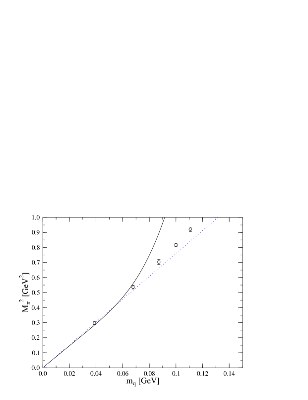
Figure 1: The square of the pion mass versus the quark mass. jlqcd data for $N_{f}=2$ are compared with the Gell-Mann–Oakes–Renner relation (dotted line) and chiral perturbation theory (full line).

For the pion decay constant $F_{\pi}$ (normalised such that the physical value is $92.4\,\mbox{MeV}$) chiral perturbation theory yields (see, e.g., Colangelo et al. 2001)

$$F_{\pi}=F\left\{1+x\hat{\ell}_{4}-\mbox{\small$\frac{5}{4}$}x^{2}\hat{\ell}_{F}^{2}+x^{2}k_{F}+O(x^{3})\right\}$$ (3)

with

$$\hat{\ell}_{F}=\frac{1}{30}(14\hat{\ell}_{1}+16\hat{\ell}_{2}+6\hat{\ell}_{3}-6\hat{\ell}_{4}+23)=\ln\frac{\Lambda_{F}^{2}}{M^{2}}\,.$$ (4)

Again, the analytic contributions $O(x^{2})$ (proportional to $k_{F}$) are expected to be small. In Fig. 2 we compare this formula with preliminary data from the ukqcd and qcdsf collaborations. Motivated by our observation that the Gell-Mann–Oakes–Renner relation works so well, we replace $M$ by $M_{\pi}$. Thus we avoid the problem of renormalising the quark mass. Choosing $F=0.0862\,\mbox{GeV}$, $k_{F}=-0.5$, $\Lambda_{4}=1.12\,\mbox{GeV}$, $\Lambda_{F}=0.67\,\mbox{GeV}$ (consistent with phenomenology) we obtain the full curve in Fig. 2, which connects the physical point with the data for the lowest mass but does not describe the data at larger masses. It is however reassuring that for masses up to the first Monte Carlo points the chiral expansion seems to be well-convergent: The dotted curve, which corresponds to $F_{\pi}=F\{1+x\hat{\ell}_{4}\}$, does not deviate dramatically from the full curve in this region.

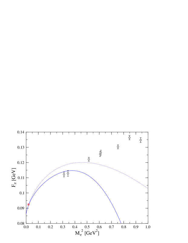
Figure 2: Preliminary data ($N_{f}=2$) for the pion decay constant compared with chiral perturbation theory at different orders. The asterisk indicates the physical point.

5 Including baryons

The nucleon mass $m_{N}$ does not vanish even in the chiral limit. Indeed $m_{N}\gg M_{\pi}$, and a non-relativistic treatment of the nucleon field seems reasonable. This leads to the so-called heavy-baryon chiral perturbation theory (hbchpt). A relativistic formulation of chiral perturbation theory in the baryon sector has been given by Becher and Leutwyler (1999). In both cases the physical picture is that of a (heavy) nucleon core surrounded by a cloud of light pions. This is rather different from the situation for the pion, and hence the behaviour of the chiral expansion in the nucleon sector need not be similar to that in the pion sector.

In Becher’s and Leutwyler’s formulation one obtains for the nucleon mass (Becher and Leutwyler 1999, Procura et al. 2004)

$$\begin{array}[]{l}\displaystyle m_{N}=m_{0}-4c_{1}M_{\pi}^{2}-\frac{3(g_{A}^{0})^{2}}{32\pi F^{2}}M_{\pi}^{3}+\left[e_{1}^{r}(\lambda)-\frac{3}{64\pi^{2}F^{2}}\left(\frac{(g_{A}^{0})^{2}}{m_{0}}-\frac{c_{2}}{2}\right)\right.\\[22.76228pt] \displaystyle\hskip 2.84544pt\left.{}-\frac{3}{32\pi^{2}F^{2}}\left(\frac{(g_{A}^{0})^{2}}{m_{0}}-8c_{1}+c_{2}+4c_{3}\right)\ln{\frac{M_{\pi}}{\lambda}}\right]M_{\pi}^{4}+\frac{3(g_{A}^{0})^{2}}{256\pi F^{2}m_{0}^{2}}M_{\pi}^{5}+O(M_{\pi}^{6})\,.\end{array}$$ (5)

Here we have again identified $M_{\pi}^{2}=M^{2}=2Bm_{q}$, $\lambda$ is the renormalisation scale, $m_{0}$ and $g_{A}^{0}$ are the mass and the axial charge of the nucleon in the chiral limit, $c_{1}$, $c_{2}$, $c_{3}$ denote coupling constants from the effective Lagrangian, and $e_{1}^{r}(\lambda)$ is a counterterm.

Hadron masses for $N_{f}=2$ have been published by the cp-pacs collaboration (Ali Khan et al. 2002), the jlqcd collaboration (Aoki et al. 2003) as well as the ukqcd and qcdsf collaborations (Allton et al. 2002, Ali Khan et al. 2004a). We have selected results obtained on (relatively) large and fine lattices to compare with chiral perturbation theory. More precisely, we have considered masses from simulations with $a<0.15\,\mbox{fm}$, $M_{\pi}<800\,\mbox{MeV}$ and $M_{\pi}L>5$. These ten data points were fitted with Eq. (5) where $g_{A}^{0}$, $F$, $c_{2}$ and $c_{3}$ were fixed to phenomenologically reasonable values while $m_{0}$, $c_{1}$ and $e_{1}^{r}(\lambda=1\,\mbox{GeV})$ were the fit parameters. For more details see (Ali Khan et al. 2004a). The fit curve and the data points are shown in Fig. 3. It is first of all remarkable that the masses obtained by different collaborations with different lattice actions and algorithms fall (to rather good accuracy) onto a single curve. Furthermore, the fit parameters are very well compatible with phenomenology, in particular, $c_{1}$ is about $-1\,\mbox{GeV}^{-1}$ and the fit curve comes quite close to the physical point. On the other hand, Eq. (5) seems to work up to surprisingly large masses.

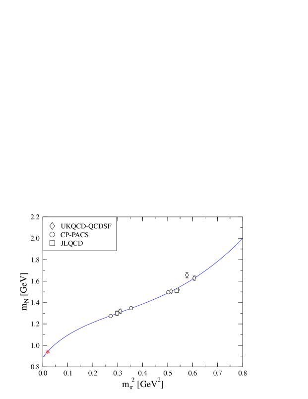
Figure 3: Nucleon mass data for $N_{f}=2$ on (relatively) large and fine lattices. The asterisk indicates the physical point. The curve corresponds to the fit mentioned in the text.

6 Axial charge of the nucleon

The quark-mass dependence of the axial charge (or axial-vector coupling constant) $g_{A}$ of the nucleon has been studied by Hemmert et al. (2003) within the framework of the so-called small-scale expansion. This is an extension of hbchpt which includes explicit $\Delta(1232)$ degrees of freedom.

In the small-scale expansion the expansion parameter is usually called $\epsilon$, and one finds in $O(\epsilon^{3})$:

$$\begin{array}[]{l}\displaystyle g_{A}(M_{\pi}^{2})=g^{0}_{A}-\frac{(g^{0}_{A})^{3}M_{\pi}^{2}}{16\pi^{2}F^{2}}\\ \displaystyle\quad{}+4\left\{C^{SSE}(\lambda)+\frac{c_{A}^{2}}{4\pi^{2}F^{2}}\left[\frac{155}{972}\,g_{1}-\frac{17}{36}\,g^{0}_{A}\right]+\gamma^{SSE}\ln{\frac{M_{\pi}}{\lambda}}\right\}M_{\pi}^{2}\\ \displaystyle\quad{}+\frac{4c_{A}^{2}g^{0}_{A}}{27\pi F^{2}\Delta}M_{\pi}^{3}+\frac{8}{27\pi^{2}F^{2}}\;c_{A}^{2}g^{0}_{A}M_{\pi}^{2}\sqrt{1-\frac{M_{\pi}^{2}}{\Delta^{2}}}\,\ln{R}\\ \displaystyle\quad{}+\frac{c_{A}^{2}\Delta^{2}}{81\pi^{2}F^{2}}\left(25g_{1}-57g_{A}^{0}\right)\left\{\ln\left[\frac{2\Delta}{M_{\pi}}\right]-\sqrt{1-\frac{M_{\pi}^{2}}{\Delta^{2}}}\ln R\right\}+O(\epsilon^{4})\end{array}$$ (6)

with

$$\gamma^{SSE}=\frac{1}{16\pi^{2}F^{2}}\left[\frac{50}{81}\,c_{A}^{2}g_{1}-\frac{1}{2}\,g_{A}^{0}-\frac{2}{9}\,c_{A}^{2}g_{A}^{0}-(g_{A}^{0})^{3}\right]\,,\,R=\frac{\Delta}{M_{\pi}}+\sqrt{\frac{\Delta^{2}}{M_{\pi}^{2}}-1}\,.$$ (7)

The new parameters appearing here are $g_{A}^{0}$ (the value of $g_{A}$ in the chiral limit), $\Delta$ (the nucleon $\Delta$ mass splitting in the chiral limit), $c_{A}$, $g_{1}$ (the $N\Delta$ and $\Delta\Delta$ axial coupling constants), and $C^{SSE}(\lambda)$ (a counterterm at the renormalisation scale $\lambda$). Hemmert et al. (2003) find that for reasonable values of the parameters the formula (6) is able to describe the rather weak mass dependence of the Monte Carlo data as well as the physical point.

7 Chiral effective field theory in a finite volume

Presently, lattice qcd simulations are not only restricted to unphysical quark masses, but also to relatively small (spatial) volumes, usually with periodic boundary conditions. While simulations at the physical quark masses might be possible some day, it will take a bit longer before the ideal case of an infinite volume simulation can be realised. In the meantime we can take advantage of the fact that the chiral effective Lagrangian is volume independent for periodic boundary conditions (Gasser and Leutwyler 1988). So the same Lagrangian governs the quark-mass as well as the volume dependence, and additional information on the coupling constants can be extracted from finite size effects. This description of the finite size effects should work as long as they result from the deformation of the pion cloud in the finite volume, i.e. as long as $L$ is not too small. After all, it is the pion propagation that is predominantly affected by the finite volume, because the pion is the lightest particle in the theory. Treating $L^{-1}$ as a quantity of order $p$ like $M_{\pi}$ we arrive at the so-called $p$ expansion (Gasser and Leutwyler 1987). This is to be distinguished from the $\epsilon$ expansion, where $L^{-1}=O(\epsilon)$, $M_{\pi}=O(\epsilon^{2})$ with a small parameter $\epsilon$.

In more technical terms, the finite volume (with periodic boundary conditions) discretises the allowed momenta such that the momentum components are restricted to integer multiples of $2\pi/L$. So the loop integrals of chpt become sums. On the other hand, we can interpret the resulting expressions in the following way. In a finite volume a pion emitted from a nucleon can not only be reabsorbed by the same nucleon, but also by one of the periodic images of the original nucleon at a distance which is an integer multiple of $L$ in each of the finite directions. From this point of view the finite size effects arise from pions travelling around the volume once, twice, … in a given direction, and each crossing of the boundary leads (roughly) to a factor $\exp(-M_{\pi}L)$ in the final contribution.

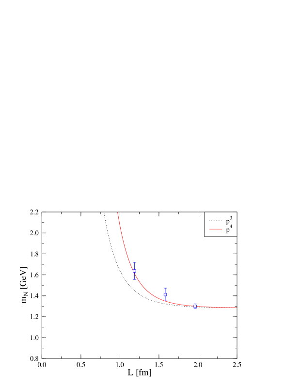
Figure 4: Volume dependence of the nucleon mass for $M_{\pi}=545\,\mbox{MeV}$. The dotted curve shows the contribution of the $p^{3}$ term, while the solid curve includes also the $p^{4}$ correction.

As an example, let us consider the nucleon mass in relativistic baryon chpt. Then the nucleon mass in a spatial box of length $L$, but for an infinite extent in time direction, can be written as

$$m_{N}(L)=m_{N}(\infty)+\Delta_{a}(L)+\Delta_{b}(L)+O(p^{5}),$$ (8)

where

$$\Delta_{a}(L)=\frac{3(g_{A}^{0})^{2}m_{0}M_{\pi}^{2}}{16\pi^{2}F^{2}}\int_{0}^{\infty}\!\mathrm{d}x\,\sum_{\vec{n}\neq\vec{0}}\,K_{0}\left(L|\vec{n}|\sqrt{m_{0}^{2}x^{2}+M_{\pi}^{2}(1-x)}\right)$$ (9)

is the $O(p^{3})$ contribution to the finite size effect and

$$\Delta_{b}(L)=\frac{3M_{\pi}^{4}}{4\pi^{2}F^{2}}\sum_{\vec{n}\neq\vec{0}}\left[(2c_{1}-c_{3})\frac{K_{1}(L|\vec{n}|M_{\pi})}{L|\vec{n}|M_{\pi}}+c_{2}\frac{K_{2}(L|\vec{n}|M_{\pi})}{(L|\vec{n}|M_{\pi})^{2}}\right]$$ (10)

is the additional contribution arising at $O(p^{4})$. Here $n_{i}$ can be interpreted as the number of times the pion crosses the ‘boundary’ of the box in the $i$ direction. Note that the finite volume does not introduce any new coupling constant. For a comparison with Monte Carlo data we evaluate the finite size corrections using the parameters from the fit discussed in Section 5, choose $m_{N}(\infty)$ such that $m_{N}(L)$ on the largest lattice agrees with the Monte Carlo value and take for $M_{\pi}$ the value from the largest lattice. This leads to a surprisingly good agreement with the Monte Carlo masses, as is shown for $M_{\pi}=545\,\mbox{MeV}$ in Fig. 4 using jlqcd data. Even for larger pion masses the formula reproduces the finite size effects quite well (Ali Khan et al. 2004a). This lends further support to the fit shown in Fig. 3.

In the case of the pion mass the leading finite volume correction has already been known for some time (Gasser and Leutwyler 1987):

$$M_{\pi}(L)=M_{\pi}\left\{1+\frac{M_{\pi}^{2}}{(4\pi F_{\pi})^{2}}\sum_{\vec{n}\neq\vec{0}}\,\frac{K_{1}(L|\vec{n}|M_{\pi})}{L|\vec{n}|M_{\pi}}+O(M_{\pi}^{4})\right\}\,.$$ (11)

Moreover, neglecting pions which travel around the box more than once ($|\vec{n}|>1$) Lüscher (1986) has expressed the finite volume correction in terms of the $\pi\pi$ forward scattering amplitude $F(\nu)$, $\nu=(s-u)/(4M_{\pi})$:

$$M_{\pi}(L)-M_{\pi}=-\frac{3}{16\pi^{2}M_{\pi}L}\int_{-\infty}^{\infty}\!\mathrm{d}y\,F(\mathrm{i}y)\mathrm{e}^{-\sqrt{M_{\pi}^{2}+y^{2}}L}\,.$$ (12)

The chiral expansion of $F(\nu)$ is known to $O(M_{\pi}^{6})$ and the corresponding coupling constants are reasonably well determined. Using this information one can work out the volume dependence of $M_{\pi}$ predicted by Eq. (12) (Colangelo and Dürr 2004). The non-leading terms of the chiral expansion give non-negligible contributions, still the finite size effects are considerably underestimated by this approach, at least for $M_{\pi}>500\,\mbox{MeV}$. Probably terms with $|\vec{n}|>1$ are important for smaller volumes, which is certainly the case in Eq. (11). However, Eq. (11) alone predicts even smaller finite size effects than Eq. (12). So it seems that one would need higher orders in the chiral expansion as well as pions propagating around the volume more than once, and the present understanding of the finite size effects for $M_{\pi}$ is unsatisfactory. For another investigation of hadron masses in a finite volume see (Orth et al. 2004).

The volume dependence of $g_{A}$ has recently attracted much interest. First calculations in chiral perturbation theory have been performed by Beane and Savage (2004). However, at the masses used in current simulations these leading-order formulae do not even reproduce the sign of the finite size effects observed in the Monte Carlo data, see, e.g., (Ali Khan et al. 2004b), (Sasaki et al. 2003). It remains to be seen whether more advanced calculations in cheft can solve this discrepancy or whether lower quark masses are required.

8 Conclusions

What has been described here, are only the first steps of an ongoing effort to combine calculations in cheft and lattice simulations. The overall impression is that the range of quark masses that can be used in actual Monte Carlo computations is beginning to overlap with the region of applicability of chpt. In favourable cases this overlap seems to be so large that meaningful fits are possible. Although fits without phenomenological input are still beyond reach, interesting information on (effective) coupling constants can already be extracted. In most cases the leading chiral logarithm appears to be dominating only for rather small quark masses. Thus cheft should be pushed to higher orders while on the lattice side results for lower quark masses are eagerly awaited.

Acknowledgements

The studies reported in this paper have been performed within the qcdsf-ukqcd collaboration. I wish to thank all my colleagues who have contributed to this effort, in particular A. Ali Khan, Ph. Hägler, T.R. Hemmert, R. Horsley, A.C. Irving, H. Perlt, D. Pleiter, P.E.L. Rakow, A. Schäfer, G. Schierholz, A. Schiller, H. Stüben and J.M. Zanotti.

The numerical calculations have been performed on the Hitachi sr8000 at lrz (Munich), on the Cray t3e at epcc (Edinburgh) and on the apemille at nic/desy (Zeuthen). This work has been supported in part by the dfg (Forschergruppe Gitter-Hadronen-Phänomenologie) and by the eu Integrated Infrastructure Initiative ‘Hadron Physics’ as well as ‘Study of Strongly Interactive Matter’.

References

Ali Khan A et al. , 2002, Phys Rev D 65 054505;  67 059901 (E).

Ali Khan A et al. , 2004a, Nucl Phys B  689 175.

Ali Khan A et al. , 2004b, arXiv:hep-lat/0409161.

Allton C R et al. , 2002, Phys Rev D 65 054502.

Aoki S et al. , 2003, Phys Rev D 68 054502.

Bär O, 2004, arXiv:hep-ph/0409123.

Beane S R and Savage M J, 2004, arXiv:hep-ph/0404131.

Becher T and Leutwyler H, 1999, Eur Phys J C  9 643.

Colangelo G, 2004, arXiv:hep-ph/0409111.

Colangelo G and Dürr S, 2004, Eur Phys J C  33 543.

Colangelo G, Gasser J, and Leutwyler H, 2001, Nucl Phys B  603 125.

Dürr S, 2003, Eur Phys J C  29 383.

Gasser J and Leutwyler H, 1987, Phys Lett B  184 83.

Gasser J and Leutwyler H, 1988, Nucl Phys B  307 763.

Göckeler M et al. , 2004, arXiv:hep-ph/0409312.

Hemmert T R, Procura M, and Weise W, 2003, Phys Rev D 68 075009.

Leinweber D B, Thomas A W, and Young R D, 2004, Phys Rev Lett 92 242002.

Leutwyler H, 2000, arXiv:hep-ph/0008124.

Lüscher M, 1986, Commun Math Phys  104 177.

Meiner U, 2000, arXiv:hep-ph/0007092.

Orth B, Lippert T, and Schilling K, 2004, Nucl Phys Proc Suppl  129 173.

Procura M, Hemmert T R, and Weise W, 2004, Phys Rev D 69 034505.

Sasaki S, Orginos K, Ohta S, and Blum T, 2003, Phys Rev D 68 054509.

Young R D, Leinweber D B, and Thomas A W, 2004, Nucl Phys Proc Suppl  128 227.