SWAT/04/419

December 2004

Lattice Study of Anisotropic QED₃

Simon Hands and Iorwerth Owain Thomas

Department of Physics, University of Wales Swansea,

Singleton Park, Swansea SA2 8PP, U.K.

Abstract

We present results from a Monte Carlo simulation of non-compact lattice QED in 3 dimensions on a $16^{3}$ lattice in which an explicit anisotropy between $x$ and $y$ hopping terms has been introduced into the action. This formulation is inspired by recent formulations of anisotropic QED₃ as an effective theory of the non-superconducting portion of the cuprate phase diagram, with relativistic fermion degrees of freedom defined near the nodes of the gap function on the Fermi surface, the anisotropy encapsulating the different Fermi and Gap velocities at the node, and the massless photon degrees of freedom reproducing the dynamics of the phase disorder of the superconducting order parameter. Using a parameter set corresponding in the isotropic limit to broken chiral symmetry (in field theory language) or a spin density wave (in condensed matter physics language), our results show that the renormalised anisotropy, defined in terms of the ratio of correlation lengths of gauge invariant bound states in the $x$ and $y$ directions, exceeds the explicit anisotropy $\kappa$ introduced in the lattice action, implying in contrast to recent analytic results that anisotropy is a relevant deformation of QED₃. There also appears to be a chiral symmetry restoring phase transition at $\kappa_{c}\simeq 4.5$, implying that the pseudogap phase persists down to $T=0$ in the cuprate phase diagram.

PACS: 11.10.Kk, 11.15.Ha, 71.27.+a, 74.25.Dw

Keywords: lattice gauge theory, cuprate, phase diagram, pseudogap

1 Introduction

The phase diagram of the superconducting cuprate compounds in the $(x,T)$ plane, where $x$ denotes the doping, or fraction of holes per CuO₂ unit, continues to be the object of much study, both experimental and theoretical. A schematic version is shown in Figure 1 [1].

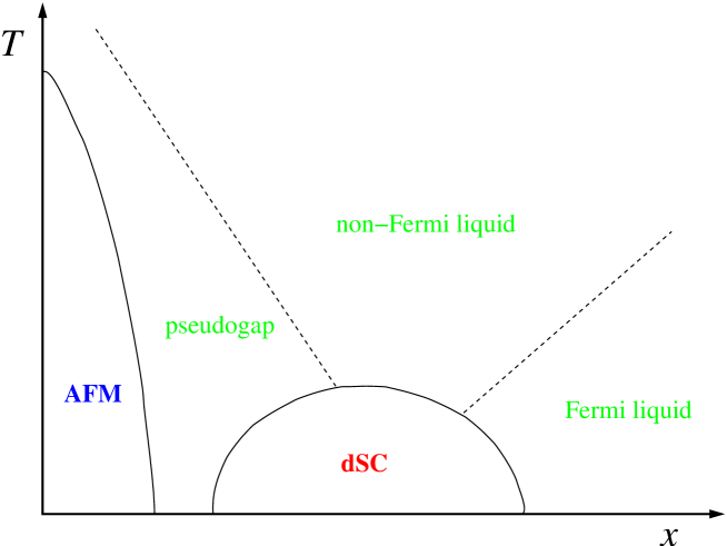
Figure 1: (Color online) Schematic phase diagram for cuprate superconductors

Around $x\sim 0.2$, so-called optimal doping, there is a superconducting dSC phase extending to temperatures as high as $T\sim 50$K. The superconductivity is believed to be an essentially two-dimensional phenomenon, being confined to the CuO₂ planes, and the gap function $\Delta(\vec{k})$ is characterised by $d$-wave symmetry, thus having two pairs of nodes on the one-dimensional Fermi surface. For $x\approx 0$ the compound is an insulating anti-ferromagnet, and as $x$ increases in this AFM phase the order smoothly evolves into a spin-density wave characterised by a wavevector $\vec{K}$ whose magnitude decreases with $x$.

In some sense the “normal” phase is more strange. While in the over-doped regime the behaviour is that of a normal metal, namely a conventional Fermi liquid, as $x$ is decreased unusual non-Fermi liquid behaviour manifests itself via non-standard $T$-scaling of transport coefficients such as resistivity and themal conductivity. More mysterious still is the “pseudogap” behaviour observed in the under-doped region; as one moves out of the dSC phase in the direction of increasing $T$ or decreasing $x$, studies of the spectral density distribution function at fixed momentum show the quasiparticle pole of the superconductor (correponding to a well-defined excitation of energy $\Delta$ above the Fermi energy) diminish in strength, but the magnitude of the energy gap $|\Delta|$ remain non-zero even in the non-superconducting region. This spectral depletion can persist up to $T\sim 150$K [2].

It should be stressed that while AFM and dSC both have well-defined order parameters, and hence are separated from the rest of the phase diagram by solid lines in Figure 1, the status of the dashed lines separating the “normal” phase into three regions is currently much less clear. Nonetheless, there have been several attempts to formulate a theoretical description of the pseudogap region. A particularly interesting programme, starting from established properties of the dSC phase, derives an effective theory which resembles QED in 2+1 dimensions, but having spatial anisotropy in the covariant derivatives [3, 4]. The starting point is the Bogoliubov – de Gennes model for $d$-wave quasiparticles in the dSC phase, which in Euclidean metric (corresponding to the imaginary time formalism in many body theory) has action

$$S = T\sum_{\vec{k},\sigma,\omega_{n}}\biggl{[}(i\omega_{n}-\xi_{\vec{k}})c^{\dagger}_{\sigma}(\vec{k},\omega_{n})c_{\sigma}(\vec{k},\omega_{n})$$ (1)

$$- {\sigma\over 2}\left(\Delta(\vec{k})c^{\dagger}_{\sigma}(\vec{k},\omega_{n})c^{\dagger}_{-\sigma}(-\vec{k},-\omega_{n})-\Delta^{\dagger}(\vec{k})c_{\sigma}(\vec{k},\omega_{n})c_{-\sigma}(-\vec{k},-\omega_{n})\right)\biggr{]},$$

where $c^{\dagger},c$ are creation and annihilation operators for electrons with spin $\sigma=\pm 1$, and $\omega_{n}=(2n-1)\pi T$ are the allowed Matsubara frequencies. The function $\xi_{\vec{k}}$ is the energy of a free quasiparticle, which thus vanishes for $\vec{k}$ on the Fermi surface, and $\Delta(\vec{k})$ is the gap function, which can be thought of as a self-consistent pairing field. The requirement of $d$-wave symmetry implies that $\Delta(\vec{k})=0$ at four special node momenta $\vec{k}=\pm\vec{K}_{1},\pm\vec{K}_{2}$ with $\vec{K}_{1}.\vec{K}_{2}=0$. If we choose axes such that $\vec{K}_{1}\parallel\hat{x}$, $\vec{K}_{2}\parallel\hat{y}$, and write $\vec{k}=\vec{K}_{i}+\vec{q}$, then in the vicinity of the “1” nodes it is possible to linearise as

$$\xi_{\vec{k}}=v_{F}q_{x}+O(q^{2})\;\;\;\;;\;\;\;\;\Delta(\vec{k})=v_{\Delta}q_{y}+O(q^{2})$$ (2)

and near the “2” nodes as

$$\xi_{\vec{k}}=v_{F}q_{y}+O(q^{2})\;\;\;\;;\;\;\;\;\Delta(\vec{k})=v_{\Delta}q_{x}+O(q^{2}),$$ (3)

where the parameters $v_{F}$ and $v_{\Delta}$ are the Fermi and Gap velocities respectively.

The next stage is to define a 4-spinor $\Psi_{i}$ at the node $i$:

$$\Psi_{i}^{\mbox{tr}}(\vec{q},\omega)=\left(c_{+}(\vec{k},\omega),c^{\dagger}_{-}(-\vec{k},-\omega),c_{+}(\vec{k}-2\vec{K}_{i},\omega),c^{\dagger}_{-}(-\vec{k}+2\vec{K}_{i},-\omega)\right).$$ (4)

The association of different spinor components with different points in $k$-space is well-known to workers in lattice QCD familiar with the staggered fermion formulation [5]. It is now possible to recast the low energy limit of the kinetic term of (1) in relativistic garb:

$$S=\int d^{2}r\int_{0}^{\beta}dt\bar{\Psi}_{1}[\gamma_{0}\partial_{t} + v_{F}\gamma_{1}\partial_{x}+v_{\Delta}\gamma_{2}\partial_{y}]\Psi_{1}+$$

$$\bar{\Psi}_{2}[\gamma_{0}\partial_{t} + v_{F}\gamma_{1}\partial_{y}+v_{\Delta}\gamma_{2}\partial_{x}]\Psi_{2}+O(\partial^{2},\Psi^{4})$$ (5)

where $\beta\equiv T^{-1}$, $\bar{\Psi}=\Psi^{\dagger}\gamma_{0}$, and the $4\times 4$ traceless hermitian Dirac $\gamma$-matrices obey $\{\gamma_{\mu},\gamma_{\nu}\}=2\delta_{\mu\nu}$. It is important to stress that there is no reason a priori for the anisotropy encapsulated in the ratio $v_{F}/v_{\Delta}\equiv\kappa$ to be negligble in real cuprates; a value as high as $\sim 10$ is reported in [6]. In addition, $\kappa$ increases with doping fraction $x$ [7].

To give the nodal fermions interactions, it is necessary to discuss the reason for the loss of superconducting order. The hypothesis is that the gap function can be written as $\Delta=\Delta_{0}(\vec{k})e^{i\theta(\vec{r})}$, where $\Delta_{0}$ is real, and that superconductivity is destroyed because the phase field $\theta$ becomes disordered. In two spatial dimensions non-trivial phase disorder arises through the accumulation of vortices, that is, point dislocations around which $\oint\nabla\theta.d\vec{\ell}=2n\pi$ [8]. The dSC $\to$ pseudogap transition is thus supposedly driven by vortex condensation, which preserves $|\Delta|\sim\Delta_{0}$ but ensures $\langle e^{i\theta}\rangle=0$. Now, it is possible to exploit the gauge symmetry of (1) to absorb phase fluctuations of $\Delta$ into the phases of $c,c^{\dagger}$ and hence $\Psi$. We would thus seek a theory of phase fluctuations for the $\Psi$ fields. However, since $\Delta$ represents a doubly-charged Cooper pair field, it is impossible to do thus while maintaining single valuedness, since the phase of $\Psi$ would change by only $\pi$ on circling a vortex. The solution proposed by Franz and Tešanović [9], is to partition the vortices of any particular configuration $\{\theta\}$ into two groups A & B, and then to associate the phase $\theta_{A}(\vec{r})$ associated with A vortices exclusively with the spin-up electrons, and that of the B to spin-down. It can then be shown [3, 4] that the relativistic $\Psi$ fields of (5) couple minimally to the vector-valued difference field $a_{\mu}={1\over 2}\partial_{\mu}(\theta_{A}-\theta_{B})$, which thus acts as an effective “photon” in the gauge-invariant action which results from replacing $\partial_{\mu}$ in (5) by the covariant derivative $D_{\mu}=\partial_{\mu}+ia_{\mu}$.

It immediately follows from gauge invariance, which implies that the vacuum polarisation tensor correcting $\langle a_{\mu}(p)a_{\nu}(-p)\rangle$ has the transverse form $(p^{2}\delta_{\mu\nu}-p_{\mu}p_{\nu})\Pi(p)$, that the $a_{\mu}$ excitations do not receive a mass due to quantum corrections from the $\Psi$ fields. Further arguments have been advanced [3, 4] to suggest that fluctuations in the $a_{\mu}$ field are themselves governed by the action of 2+1$d$ electrodynamics

$$S_{phot}={1\over 2g^{2}}\int d^{2}r\int_{0}^{\beta}dt(\partial_{\mu}a_{\nu}-\partial_{\nu}a_{\mu})^{2},$$ (6)

with the coupling $g$ related to the diamagnetic susceptibility $\chi$ via $g\sim\chi^{-{1\over 2}}$, or in field theoretic terms to the dual order parameter $\tilde{\Phi}$ for vortex condensation via $g\sim\langle\tilde{\Phi}\rangle$.

One way of understanding this is that in the absence of magnetic monopoles (which in 2+1$d$ are instantons) which can act as a source or sink of flux, vorticity is a topologically-conserved charge. When the ground state is such that $\langle\tilde{\Phi}\rangle\not=0$, the U(1) global symmetry for which vorticity is a Noether charge, i.e. the timelike component of a conserved current $\tilde{V}_{\mu}$, is spontaneously broken, resulting in a massless boson in the spectrum via Goldstone’s theorem. However, in 2+1$d$ this Goldstone boson is kinematically equivalent to the photon, as can be seen via, eg, the PCAC-like relation [10]

$$\langle 0|\tilde{V}_{\mu}|\mbox{1 photon},\vec{p}\rangle\propto p_{\mu}.$$ (7)

As a result of these considerations, it is natural to unite (5) and (6) and postulate a relativistic field theory, QED₃ with $N_{f}=2$ flavours of nodal fermion $\Psi$, as the appropriate effective action for low energy long wavelength excitations in the pseudogap phase – the photons $a_{\mu}$ interacting with the $\Psi$ with effective electric charge $g$.

QED₃ is an asymptotically-free theory, which means that it becomes more strongly interacting as energy scales decrease, ie. as length scales grow. The infra-red behaviour of QED₃ has long been a challenge to theory (see [11] for a brief review); in brief, the issue is whether the chiral symmetry $\Psi\mapsto e^{i\alpha\gamma_{5}}\Psi$, $\bar{\Psi}\mapsto\bar{\Psi}e^{i\alpha\gamma_{5}}$ of (5) (with $\gamma_{5}\equiv\gamma_{0}\gamma_{1}\gamma_{2}\gamma_{3}$) is spontaneously broken by a parity-invariant fermion – anti-fermion condensate $\langle\bar{\Psi}\Psi\rangle\not=0$. This is believed to happen if the number of flavours $N_{f}$ is smaller than some critical value $N_{fc}$, which has been variously estimated as taking values in the range $\raisebox{-2.15277pt}{$\ \stackrel{{\scriptstyle\textstyle<}}{{\textstyle\sim}}\ $}{3\over 2}$ to $\sim 5$. The consequence is a dynamically generated fermion mass $\Sigma$; the determination of the exact value of $N_{fc}$, and the dynamically generated ratios $\Sigma/g^{2}$ and $\langle\bar{\Psi}\Psi\rangle/g^{4}$ remain outstanding problems in non-perturbative field theory.

To understand this issue in the context of cuprates it is necessary to return to the original electron variables $c,c^{\dagger}$. If $N_{fc}>2$ then chiral symmetry is broken at $T=0$ in the long-wavelength or continuum limit. This translates into a non-vanishing value for $\langle\sum_{\sigma,i}\sigma\cos(2\vec{K}_{i}.\vec{r})c^{\dagger}_{\sigma}(\vec{r})c_{\sigma}(\vec{r})\rangle$, which is nothing but the order parameter for spin density waves characterised by wavevectors $2\vec{K}_{i}$ [4]. This implies that for sufficiently small $T$ there is a direct passage from AFM to dSC without going through an intermediate strip of the pseudogap phase, and a corresponding triple point at the intersection of AFM, dSC and normal phases for some $T>0$. If, on the other hand, $N_{fc}<2$, then we expect the pseudogap phase to persist all the way down to $T=0$, as sketched in Fig. 1. In either case, it may be possible to explain the non-Fermi liquid properties in terms of a non-perturbatively large anomalous scaling dimension for $\Psi$ in the chirally-symmetric phase of QED₃ [3].

The above discussion ignores the effects of the anisotropy $v_{F}/v_{\Delta}\equiv\kappa>1$. This has been justified by analytic treatments performed for small departures from isotropy in the limit of large-$N_{f}$ [12, 13], where it is shown anisotropy is irrelevant in the renormalisation group (RG) sense. Specifically, Ref. [12] uses a Schwinger-Dyson approach in the large-$N_{f}$ limit to study the behaviour of $\kappa$ under RG flow, finding

$${d{\kappa_{ren}}\over ds}=-{32\over{5\pi^{2}N_{f}}}(\kappa_{ren}-1)$$ (8)

where $s$ is the logarithm of the ratio of UV cutoff to physical momentum scales. This implies that for weak anisotropy ($\kappa\raisebox{-2.15277pt}{$\ \stackrel{{\scriptstyle\textstyle>}}{{\textstyle\sim}}\ $}1$) $\kappa_{ren}$ is driven to 1 under RG flow and hence $\kappa_{ren}-1$ is an irrelevant parameter, ie. $\frac{\kappa_{ren}-1}{\kappa-1}<1$. Hence, it is argued, predictions from isotropic QED₃ can be applied directly to cuprates.

The purpose of the current paper is to examine this claim for arbitrary $\kappa$ and the “physical” case $N_{f}=2$. The theoretical tool we use is lattice simulation of so-called non-compact QED, modelling the fermi degrees of freedom as staggered lattice fermions. The lattice method is fully non-perturbative, with systematically improvable errors due to a finite UV cutoff (the inverse lattice spacing $a^{-1}$), and a non-zero IR cutoff (the inverse lattice size $L^{-1}$) of a completely different nature to other approaches. The non-compact nature of the model, to be defined more fully in Sec. 2 below, has the effect of suppressing monopoles (which appear as point singularities in the phase field $a_{\mu}$), thus maintaining the masslessness of the photon [14, 15]. Lattice simulations of isotropic QED₃ have in the past been applied to the issue of $N_{fc}$: such attempts have been hampered by large finite volume effects in the continuum limit due to the massless photon, and to date the results are only able to suggest $N_{fc}>1$ [11, 16]. In this study we work away from the continuum limit at a coupling $g$ sufficiently strong that we are confident chiral symmetry is broken at $\kappa=1$, and then systematically increase $\kappa$. Further details of the lattice model and our simulation are given in Sec. 2. In Sec. 3 we present numerical results, and in particular present evidence firstly for a restoration of chiral symmetry at some critical $\kappa_{c}$, and secondly for the renormalised anisotropy $\kappa_{ren}(\kappa)>\kappa$, where $\kappa_{ren}$ is defined in terms of certain correlation lengths in differing directions, implying in contrast to the analytic results that anisotropy is a relevant deformation of QED₃. Implications for cuprate superconductivity are discussed in Sec. 4.

2 The Model and Simulation

The lattice formulation of QED with non-compact gauge fields and staggered lattice fermions is described in detail in ref. [16]. The following is an $N$ flavour staggered fermion action for QED₃ with explicit $x-y$ anisotropy:

$$S=\sum_{i=1}^{N}\sum_{x,x^{\prime}}a^{3}\bar{\chi_{i}}(x)M_{x,x^{\prime}}\chi_{i}(x^{\prime})+\frac{\beta}{2}\!\!\sum_{x,\mu<\nu}\!\!a^{3}\Theta_{\mu\nu}^{2}(x)$$ (9)

The fermion matrix $M_{x,x^{\prime}}$ is defined as follows:

$$M_{x,x^{\prime}}={1\over 2a}\sum_{\mu=1}^{3}\xi_{\mu}(x)[\delta_{x^{\prime},x+\hat{\mu}}U_{x\mu}-\delta_{x^{\prime},x-\hat{\mu}}U_{x^{\prime}\mu}^{\dagger}]+m\delta_{\mu\nu}$$ (10)

with $\xi_{\mu}$ given by

$$\xi_{\mu}(x)=\lambda_{\mu}\eta_{\mu}(x)$$ (11)

and $\eta_{\mu}(x)=(-1)^{x_{1}+...+x_{\mu-1}}$, where $x_{1}=x$, $x_{2}=y$ and $x_{3}=t$, is the Kawomoto-Smit phase of the staggered fermion field. The $\lambda_{\mu}$ are anisotropy factors, to which we assign the following values: $\lambda_{x}=\kappa^{-\frac{1}{2}}$, $\lambda_{y}=\kappa^{\frac{1}{2}}$, $\lambda_{t}=1$. The purpose of the phase factors is to ensure that in the isotropic limit $\lambda=1$ the action describes relativistic covariant fermions [5].

If the photon-like degree of freedom $\theta_{\mu}(x)$ is defined on the link connecting site $x$ to site $x+\hat{\mu}$, then $U_{x\mu}\equiv\exp(ia\theta_{x\mu})$ in (10) is the parallel transporter defining the gauge interaction with the fermions, and we have a non-compact gauge action given by

$$\Theta_{\mu\nu}(x)={1\over a}[\Delta_{\mu}^{+}\theta_{\nu}(x)-\Delta_{\nu}^{+}\theta_{\mu}(x)].$$ (12)

The dimensionless parameter $\beta$ is given in terms of the QED coupling constant (ie. the “electron charge”) via $\beta\equiv 1/g^{2}a$, where $a$ is the lattice spacing. It is convenient to work wherever possible in units such that $a=1$. As discussed above, we use a non-compact formulation of the gauge fields because flux symmetry is not preserved in compact U(1) formulations due to instanton formation, which causes the photon in such formulations to be massive [14, 15].

If we restrict our attention to that portion of the action involving the fermion fields, then we see that the introduction of the $\lambda_{\mu}$ factors has the effect, at least at tree level, of rescaling the lattice spacing in the various directions as $a_{x}=\surd\kappa a$, $a_{y}=a/\surd\kappa$, $a_{t}=a$. In orthodox lattice QCD similar anisotropies are often introduced for technical convenience; eg. spectroscopy of highly excited states such as glueballs is considerably more efficient if $a_{t}\ll a_{x},a_{y},a_{z}$ [17]. In this case to ensure Lorentz covariance of the continuum limit it is important to check that all terms in the lattice action are formulated with the same anisotropy, which results in a fine-tuning problem once quantum corrections are introduced. For instance, implementing this programme for the action (9) would require the introduction of separate gauge coupling constants $\beta_{xt}$, $\beta_{yt}$, and $\beta_{xy}$, with a non-trivial constraint resulting from the physical requirement that eg. the speed of light for photons is the same as that for fermions. In the case at hand, though, the plaquette coupling $\beta$ is defined the same in all three planes. It is important to stress that in this case the $x-y$ anisotropy is physical, and that eg. the resulting ratio $a_{x}/a_{y}$ is an observable to be determined empirically. At tree level $a_{x}/a_{y}=\kappa$; in what follows (see Sec. 3.3.2) we define this ratio as the renormalised anisotropy $\kappa_{ren}$ and estimate it from the spatial decay of a mesonic correlation function. Rather than keep track of the various lattice spacings, we prefer to think of $\kappa$ as a parameter of the model which can be renormalised through quantum corrections. This approach was pioneered in Ref. [12], where it was shown using large-$N_{f}$ arguments that $\kappa_{ren}<\kappa$ (note that in [12] the equivalent parameter is called $\lambda$, and that our model sets their parameter $\delta$ to 1).

We set $N=1$, which yields $N_{f}=2$ fermion species in the continuum limit. An algebraic transformation exists relating the single component staggered fields $\chi,\bar{\chi}$ to four-component continuum spinors $\Psi$ [18], and in particular the chiral condensates are related via $\langle\bar{\chi}\chi\rangle=\sum_{i}\langle\bar{\Psi}_{i}\Psi_{i}\rangle$. However, we note that in the simulations presented in this paper we are working at a strong coupling ($\beta=0.2$), far from the continuum limit; this was done so that we could be reasonably confident that chiral symmetry is broken [16], allowing us to examine the effects of anisotropy on the model’s phase stucture starting from the putative AFM phase. A certain amount of caution is mandated in applying our results to the condensed matter-inspired QED₃ model (5,6), which is derived and justified in continuum terms. Further caution is warranted as the flavour structure of (10) does not entirely capture the theory of [3, 4]; in the condensed matter-inspired theory (5) the second flavour has a $v_{F}\gamma_{1}$ term in the $y$ direction and a $v_{\Delta}\gamma_{2}$ term in the $x$ direction so the two flavours have opposite anisotropies, reflecting the fact that there is no physical anisotropy in the original crystal: in our model by contrast, following the transformation to $\Psi,\bar{\Psi}$ variables the the velocity-$\gamma$ matrix structure of the first flavour would be repeated in the second, so that there is an overall anisotropy. We expect however that enough similarities between (9) and the cuprate-inspired model persist for us to make reasonable conjectures as to the behaviour of the latter system. The point will be discussed further below.

In order to aquire our results, we utilised a Hybrid Monte Carlo simulation of the action (9) with even-odd partitioning on a $16^{3}$ lattice at $\beta=0.2$, simulating for anisotropies $1\leq\kappa\leq 10$ at bare masses of $0.01\leq m\leq 0.05$. Further details can be found in [16]; here it suffices to note that the algorithm generates representative configurations of $\{\theta\}$ weighted according to the action (9) in an exact, that is to say unbiased manner. It is in principle possible to perform simulations with a lattice action corresponding more closely to the anisotropy structure of (5), but in this case simulations would have to be performed with a Hybrid Molecular Dynamics algorithm, and results would thus contain a systematic dependence on the timestep size used [16]. This algorithm would then approximate the “correct” model via a functional measure $[\mbox{det}M(\kappa)M(\kappa^{-1})]^{1\over 2}$; however, away from the continuum limit it remains an unresolved issue whether the resulting dynamics is that of a local Lagrangian field theory.

Around 1000 trajectories of mean length 1.0 were generated for each data point, and acceptance rates were generally in the region of 70-80% for $0.02\leq m\leq 0.05$ and 60-70% for $m=0.01$ (where simulations were less efficient) apart from $\kappa=10.00$, whose acceptance was over 80%.

3 Numerical Results

We performed measurements of the following parameters in our simulation: the mean gauge action $\langle{\beta\over 2}\Theta_{\mu\nu}^{2}\rangle$ separately in each $\mu\nu$ plane, the chiral condensate $\langle\bar{\chi}\chi\rangle$, the longitudinal susceptibility $\chi_{l}\equiv\partial\langle\bar{\chi}\chi\rangle/\partial m$, and the pion correlator $C_{\pi}$ in each direction, from which we extracted the pion mass ($t$ direction) and the effective masses (also known as inverse screening lengths) in both space directions $x$ and $y$.

3.1 Plaquettes

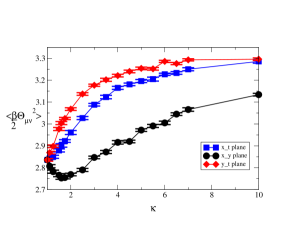
(a)

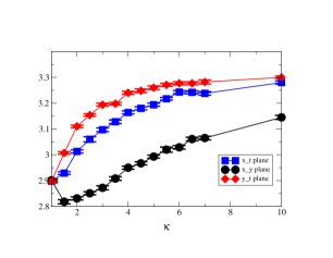
(b)

Figure 2: (Color online) Plaquette action for (a) $m=0.01$, and (b) $m=0.05$ as functions of anisotropy $\kappa$

Fig. 2 shows average gauge action values for $\kappa$ between 1 and 10 for bare fermion mass $m=0.01$ (a) and 0.05 (b). This is an important observable in exposing dynamical fermion effects: since the plaquette term $\propto\Theta^{2}$ in (9) is $\kappa$-independent, any anisotropy effect must be due to the effects of quantum corrections due to the fermion sector.

The general upward trend of the $x-t$ and $y-t$ plaquette values with $\kappa$ could plausibly be explained as a result of reduced screening of bare charge due to quantum corrections. In perturbation theory the dominant screening process is known as vacuum polarisation — virtual light $\Psi\bar{\Psi}$ pairs decrease the effective value of $g$ and hence increase the effective $\beta$; this implies that fluctuations $\langle\Theta^{2}\rangle$ are more strongly suppressed by the dynamics of (9). This can be seen by comparing the $m=0.05$ and $m=0.01$ data at $\kappa=1$. The increase of $\langle\Theta^{2}\rangle$ with $\kappa$ would therefore suggest that light $\Psi\bar{\Psi}$ pairs become less important as anisotropy increases. It will prove difficult, at first sight, to reconcile this observation with results of Sec. 3.2.

That the value of the average $x-t$ plaquette is consistently less than that in the $y-t$ plane can be explained as being due to the overall $x-y$ anisotropy of (9); in the condensed matter model (5) anisotropic effects should cancel between the two flavours. Accordingly, we can interpret the $\raisebox{-2.15277pt}{$\ \stackrel{{\scriptstyle\textstyle<}}{{\textstyle\sim}}\ $}4$% mismatch between $\langle\Theta_{xt}^{2}\rangle$ and $\langle\Theta_{yt}^{2}\rangle$ in Fig. 2 as some measure of the systematic error in our treatment.

However, the $x-y$ plane plaquettes are markedly different. First, the behaviour is non-monotonic – we observe two regimes, one for $1<\kappa\raisebox{-2.15277pt}{$\ \stackrel{{\scriptstyle\textstyle<}}{{\textstyle\sim}}\ $}1.5$, and another for $\kappa\raisebox{-2.15277pt}{$\ \stackrel{{\scriptstyle\textstyle>}}{{\textstyle\sim}}\ $}1.5$. Within the latter, we have behaviour consistent with the other two planes, but for small $\kappa$ the mean plaquette value decreases as $\kappa$ is increased. Secondly, the relative splitting between $x-y$ and $x-t$, $y-t$ is much larger, $O(10\%)$. In this case there is no symmetry argument to suggest that this splitting should vanish for dynamics based on the condensed matter model (5,6) and indeed, the approximately quadratic behaviour for small $\kappa$ suggests that some residual anisotropy effect should survive even in an $x-y$ symmetrised model, in which effects linear in $\kappa$ might be expected to cancel between the two flavours [19].

3.2 Restoration of Chiral Symmetry

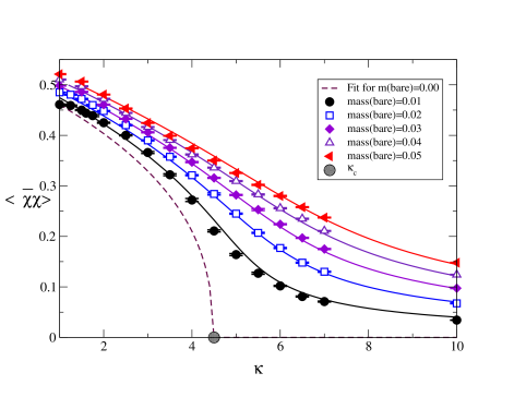
Figure 3: (Color online) Chiral condensate $\langle\bar{\chi}\chi\rangle$ versus $\kappa$. Lines denote fits to the equation of state (15)

The chiral condensate is defined in terms of the inverse fermion matrix:

$$\langle\bar{\chi}\chi\rangle=-{1\over V}{{\partial\ln Z}\over\partial m}={1\over V}\langle\mbox{tr}M^{-1}\rangle,$$ (13)

and the longitudinal susceptibility as:

$$\chi_{l}=\frac{\partial\langle\bar{\chi}\chi\rangle}{\partial m}={1\over V}[\langle\mbox{tr}M^{-1}\mbox{tr}M^{-1}\rangle-\langle\mbox{tr}M^{-1}\rangle^{2}-\langle\mbox{tr}M^{-1}M^{-1}\rangle].$$ (14)

Anisotropy effects observed within the fermion sector should also be present in the symmetrised model (5), although of course with the roles of $x$ and $y$ reversed for the second flavour.

Figures 3 and 4 depict $\langle\bar{\chi}\chi\rangle$ and $\chi_{l}$ for bare masses between 0.01 and 0.05 for various $\kappa$. Note first of all that for $\kappa\raisebox{-2.15277pt}{$\ \stackrel{{\scriptstyle\textstyle>}}{{\textstyle\sim}}\ $}1$ $\langle\bar{\chi}\chi\rangle$ varies very little as $m$ decreases, and certainly extrapolates to a non-zero value as $m\to 0$, implying the spontaneous breaking of chiral symmetry in this limit. This is consistent with the behaviour observed at strong coupling in [16, 11]. Figs. 3 and 4 both suggest a chiral symmetry restoring phase transition as $\kappa$ is increased: a drop in the value of the chiral condensate in Figure 3 (most pronounced for $m=0.01$) and, in Figure 4, a peak in the susceptibility which grows more prominent as the mass is decreased.

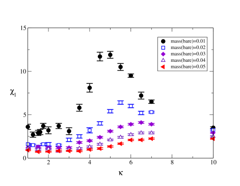
Figure 4: (Color online) $\chi_{l}$ versus $\kappa$.

We performed a fit of the $\langle\bar{\chi}\chi\rangle$ data to a hypothetical equation of state of the form

$$m=A(\kappa-\kappa_{c})\langle\bar{\chi}\chi\rangle^{\rho}+B\langle\bar{\chi}\chi\rangle^{\delta},$$ (15)

which assumes a second order phase transition at $m=0$, $\kappa=\kappa_{c}$ with conventionally-defined critical exponents $\delta$ and $\beta_{mag}=(\delta-\rho)^{-1}$ [16]. We chose to fit values of $\kappa$ from 1 to 7, as there are too few points above $\kappa=7.00$ to give a good definition of the curve. Fixing the values of the exponents $\rho$ and $\delta$ to 1 and 3 respectively gives us a mean field approximation; we find $A=0.0710(2)$, $B=1.382(6)$ and $\kappa_{c}=5.018(7)$ with a $\chi^{2}/d.o.f.$ of 72. If $\rho$ and $\delta$ are allowed to vary, we obtain $A=0.103(1)$, $B=2.75(6)$, $\kappa_{c}=4.35(2)$, $\rho=1.297(9)$ and $\delta=3.99(3)$ with a $\chi^{2}/d.o.f.$ value of 51. The latter fit is plotted as solid lines in Fig. 3, with the dashed lines denoting the equation of state in the chiral limit. Despite the large values of $\chi^{2}$, these curves seem to describe the data reasonably well; we conjecture that if a phase transition occurs, it will do so at $\kappa_{c}\approx 4.5$. A finite volume scaling study is needed before the order of the phase transition, and hence the validity of (15) can be established unambiguously.

While Figs. 3 and 4 show clear evidence of a phase transition across which $\langle\chi\chi\rangle$ decreases dramatically, it is too early to draw conclusions regarding its precise nature. For a second order transition, $\chi_{l}$ should diverge at the critical anisotropy in the chiral limit $m\to 0$. However, without a comparison of data from different volumes a first order transition cannot be excluded. In the current context the implications are profound: a second order transition would lead us to expect $\langle\bar{\chi}\chi\rangle=0$ for $m=0$, $\kappa>\kappa_{c}$, implying $N_{fc}<2$ in this regime, whereas if the transition is first order it remains conceivable that $\langle\bar{\chi}\chi\rangle\neq 0$ is small but non-zero, and hence $N_{fc}>2$. Caution is required because simulations of isotropic QED₃ with $N_{f}=2$ cannot exclude a very small dimensionless condensate $\beta^{2}\langle\bar{\chi}\chi\rangle<10^{-4}$ in the continuum limit [11], invisible on the scale of Fig. 3, but nonetheless perfectly consistent with recent analytical estimates [20].

3.3 Pion Correlation Functions and Spectroscopy

In this subsection we focus on the correlation functions

$$C_{\pi\mu}(x_{\mu})=\sum_{\nu\not=\mu}\sum_{x_{\nu}}\langle\bar{\chi}\varepsilon\chi(0)\bar{\chi}\varepsilon\chi(x)\rangle,$$ (16)

where the phase $\varepsilon(x)\equiv(-1)^{\sum_{\mu}x_{\mu}}$. In the isotropic limit $\kappa=1$ on a symmetric $L^{3}$ lattice all the $C_{\pi\mu}$ coincide. When chiral symmetry is spontaneously broken it can be shown that the correlator is dominated by one of $N^{2}$ pseudoscalar approximate Goldstone boson poles whose mass $m_{\pi}^{2}\propto m$. By analogy with particle physics we refer to such states as pions; in continuum notation they are interpolated by the operator $\bar{\Psi}\gamma_{5}\Psi$ [21]. Now, in Euclidean quantum field theory for sufficently large separation $|x_{\mu}|$ the correlator can generally be fitted by the form

$$C_{\pi\mu}(x_{\mu})=A(e^{-m_{\pi\mu}x_{\mu}}+e^{-m_{\pi\mu}(L_{\mu}-x_{\mu})}),$$ (17)

where $L_{\mu}$ is the extent of the lattice in the $\mu$ direction. For $\mu=t$ the decay parameter $m_{\pi t}$ is the pion mass, ie. the excitation energy to create a pion at rest, whereas for $\mu=x,y$ the corresponding quantities are identified as inverse screening lengths. Of course, on an isotropic symmetric lattice corresponding to $T\approx 0$ all three coincide, but in our system with explicit $x-y$ anisotropy, $m_{\pi x}$, $m_{\pi y}$ and $m_{\pi t}$ are all distinct.

3.3.1 Pion correlators in the time direction

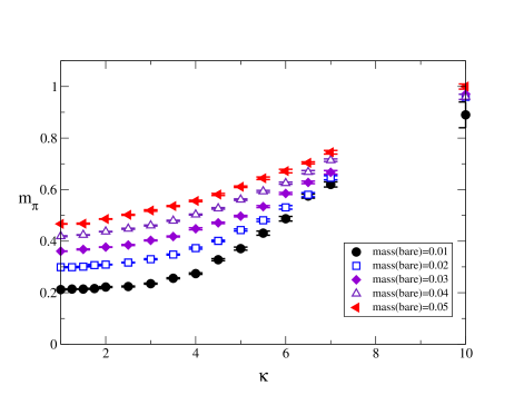
Figure 5: (Color online) $m_{\pi t}$ as $\kappa$ increases.

Figure 5 shows the variation of $m_{\pi t}$ as $\kappa$ is increased. These values were extracted from the timeslice pion propagator (16) via least squares fitting to (17). Some caveats must be offered regarding this data: it is apparent that for the very lightest pions the masses were too small for the lattice size (ie. $L\gg m_{\pi}^{-1}$ is not satisfied), meaning that we could not use an effective mass plot in order to estimate the ideal fitting window for each mass. Instead, we chose the fit window that provided the best $\chi^{2}$ value and that produced a curve that passed through the error bars of as many of the propagator data points as possible. Because of this, a table listing all the data points, their $\frac{\chi^{2}}{d.o.f}$ values and their fit windows is given below (table 1). Despite the uncertainty this procedure yields in the absolute values of $m_{\pi t}$, the trends found in the data are not artefacts of the fit window chosen, coinciding for masses where the fit window is more or less stable ($m=0.01$) as well as those where it is less so (eg. $m=0.05$).

It is clear from Figure 5 that $m_{\pi t}$ for all $m$ increases with $\kappa$ is increased, most dramatically for $\kappa\raisebox{-2.15277pt}{$\ \stackrel{{\scriptstyle\textstyle>}}{{\textstyle\sim}}\ $}4$, where the $m=0.01$ data show a perceptible kink. It appears therefore that in the chiral limit $m\to 0$ we have two regimes, one where $m_{\pi t}$ is relatively insensitive to anisotropy, and one where $m_{\pi t}$ increases approximately linearly with $\kappa$. It is tempting to identify the boundary between these two regimes with $\kappa_{c}$ of the last section – indeed, non-analytic behaviour across a phase transition should be expected since the pion is a Goldstone mode of the broken phase $\kappa<\kappa_{c}$. The linear behaviour of $m_{\pi t}(\kappa)$ for all masses in the region $5\raisebox{-2.15277pt}{$\ \stackrel{{\scriptstyle\textstyle<}}{{\textstyle\sim}}\ $}\kappa\raisebox{-2.15277pt}{$\ \stackrel{{\scriptstyle\textstyle<}}{{\textstyle\sim}}\ $}7$ is not as yet understood.

The behaviour of pions at low energies can be described by the non-linear sigma model:

$$S_{NLSM}=\frac{f_{\pi}^{2}}{2}\int d^{3}x(\partial_{\mu}U)^{\dagger}(\partial^{\mu}U),$$ (18)

where $U(x)\equiv\exp(i\pi(x)/f_{\pi})$ is a unitary matrix of the chiral group $G$ and the coupling $f_{\pi}$, known as the the pion decay constant, parametrises the strength of pion self-interactions, which become weak in the limit $k\to 0$.

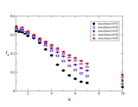
Figure 6: (Color online) $f_{\pi}$ as $\kappa$ increases.

We may calculate $f_{\pi}$ for various $\kappa$ by relating $m_{\pi}$ and $\langle\bar{\chi}\chi\rangle$ using the Gell-Mann-Oakes-Renner relation [22],

$$m_{\pi}^{2}f_{\pi}^{2}=m\langle\bar{\chi}\chi\rangle$$ (19)

The results are plotted in Figure 6. They track the $\langle\bar{\chi}\chi\rangle$ results of Figure 3 very closely; this is perhaps unsuprising, as the chiral condensate was used in our calculation, and $m_{\pi t}$ varies little for $\kappa<\kappa_{c}$.

3.3.2 Pion correlators in the x and y directions

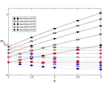
Figure 7: (Color online) Screening masses $m_{\pi x}$ (solid), $m_{\pi y}$ (dotted), and the geometric mean $\sqrt{m_{\pi x}m_{\pi y}}$ (dot-dashed), versus $\kappa$.

Figure  7 summarises the variation in the effective pion mass in the $x$ and $y$ directions, as obtained by fitting $C_{\pi x,y}$ data to the form (17). We were unable to fit for $m_{\pi y}$ beyond $\kappa=3.00$; the propagator took on a saw-tooth form consistent with the pion correlation length being infinite for all practical purposes, ie $m_{\pi y}\ll L_{y}^{-1}$. Tables 2 and 3 give fit windows and $\frac{\chi^{2}}{d.o.f}$ for each point.

The data shows $m_{\pi x}$ increasing with $\kappa$, and $m_{\pi y}$ decreasing. This is not unexpected; naively restoring explicit factors of lattice spacing we expect $m_{\pi\mu}=M_{\pi}a_{\mu}=\lambda_{\mu}^{-1}M_{\pi}a$ where $M_{\pi}$ is the expected dimensionful pion mass assuming no physical effect as a result of aniostropy. This implies that the mass pole of the propagator is shifted by a factor of $\kappa^{\frac{1}{2}}$ in the $x$ direction and by $\kappa^{-\frac{1}{2}}$ in the $y$ direction. Indeed, the geometric mean $\sqrt{m_{\pi x}m_{\pi y}}$ is approximately independent of $\kappa$, suggesting that the results can be explained entirely in terms of equal and opposite anisotropies, ie. $a_{x}a_{y}=a^{2}$.

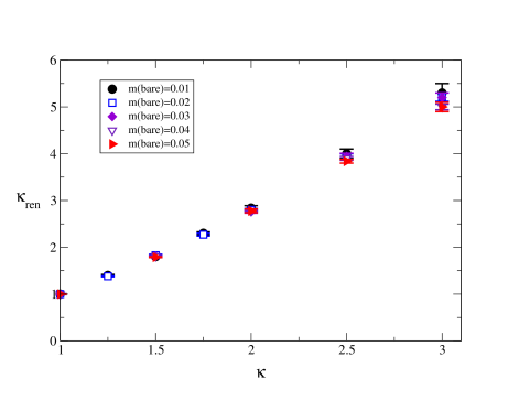
Figure 8: (Color online) $\kappa_{ren}$ versus $\kappa$ in the accessible regime $\kappa\leq 3$.

However, we should consider the possiblity that as a result of dynamical effects the physical anisotropy is not simply related to the “bare” anisotropy introduced in (9). We can then regard the ratio $m_{\pi x}/m_{\pi y}$ as a measure of the physical or renormalised anisotropy $\kappa_{ren}$ [23]. Figure 8 plots the resulting $\kappa_{ren}(\kappa)$; in fact $\kappa_{ren}$ is approximately described by

$${{\kappa_{ren}-1}\over{\kappa-1}}\approx 2,$$ (20)

a relation which appears remarkably insensitive to the fermion mass $m$.

Eqn. (20) implies that the physical anisotropy is greater than that in the bare theory, in direct contradiction to the analytic prediction of Lee and Herbut [12]. Our results suggest $\kappa_{ren}-1$ is relevant. Possible explanations for the discrepancy are firstly that we are not necessarily simulating at a small enough anisotropy, or sufficiently close to the continuum limit, where the results of [12] apply, and secondly, as we have stressed in Section 2, the model (9) does not quite reproduce the theory examined there.

$m$	$\kappa$	$\frac{\chi^{2}}{d.o.f}$	fit window	$m$	$\kappa$	$\frac{\chi^{2}}{d.o.f}$	fit window
0.01	1.00	1.395	1-15	0.02	1.00	1.156	1-15
	1.25	0.633	1-15		1.25	1.095	3-13
	1.50	1.118	1-15		1.50	0.900	1-15
	1.75	0.753	1-15		1.75	0.652	5-11
	2.00	1.041	3-13		2.00	1.021	2-14
	2.50	1.011	1-15		2.50	1.341	1-15
	3.00	1.332	1-15		3.00	1.167	3-13
	3.50	0.901	1-15		3.50	1.373	2-14
	4.00	1.318	1-15		4.00	1.170	4-12
	4.50	1.587	1-15		4.50	1.783	1-15
	5.00	1.197	1-15		5.00	3.112	3-13
	5.50	1.341	2-14		5.50	1.126	1-15
	6.00	1.045	2-14		6.00	0.476	2-14
	6.50	1.502	1-15		6.50	1.044	2-14
	7.00	1.592	2-14		7.00	1.090	2-14
	10.00	1.634	5-11		10.00	1.005	1-15
0.03	1.00	1.080	2-14	0.04	1.00	1.008	5-11
	1.50	1.014	4-12		1.50	0.855	2-14
	2.00	0.961	1-15		2.00	1.064	2-14
	2.50	1.298	3-13		2.50	0.811	4-12
	3.00	1.065	1-15		3.00	1.271	1-15
	3.50	1.058	3-13		3.50	0.882	1-15
	4.00	1.112	5-11		4.00	1.562	1-15
	4.50	1.684	2-14		4.50	1.045	1-15
	5.00	1.202	1-15		5.00	0.999	1-15
	5.50	1.301	1-15		5.50	0.858	3-13
	6.00	0.804	1-15		6.00	1.413	1-15
	6.50	1.166	1-15		6.50	1.076	3-13
	7.00	1.071	1-15		7.00	1.101	1-15
	10.00	1.128	4-12		10.00	0.599	1-15
0.05	1.00	0.963	3-13
	1.50	1.368	4-12
	2.00	1.521	1-15
	2.50	1.385	4-12
	3.00	0.914	5-11
	3.50	0.938	4-12
	4.00	0.716	3-13
	4.50	1.544	4-12
	5.00	1.218	2-14
	5.50	1.018	5-11
	6.00	1.003	5-11
	6.50	0.951	1-15
	7.00	0.705	2-14
	10.00	1.893	2-14

Table 1: Pion mass $m_{\pi t}$ fitting data

$m$	$\kappa$	$m_{\pi x}$	$\frac{\chi^{2}}{d.o.f}$	fit window
0.01	1.00	0.211(1)	1.073	2-14
	1.25	0.251(1)	0.927	1-15
	1.50	0.289(1)	0.636	1-15
	1.75	0.319(1)	0.742	1-15
	2.00	0.356(2)	1.214	1-15
	2.50	0.423(2)	0.975	1-15
	3.00	0.492(3)	1.735	3-13
0.02	1.00	0.298(1)	1.256	1-15
	1.25	0.352(1)	0.812	1-15
	1.50	0.400(1)	1.016	1-15
	1.75	0.448(1)	1.397	2-14
	2.00	0.498(2)	1.000	2-14
	2.50	0.585(2)	1.313	2-14
	3.00	0.673(2)	0.709	1-15
0.03	1.00	0.364(1)	1.124	1-15
	1.50	0.486(1)	0.671	2-14
	2.00	0.600(2)	0.914	4-12
	2.50	0.710(2)	1.115	1-15
	3.00	0.810(3)	1.074	5-11
0.04	1.00	0.467(1)	1.049	1-15
	1.50	0.621(1)	0.960	4-12
	2.00	0.765(3)	0.940	6-10
	2.50	0.897(2)	1.044	1-15
	3.00	1.024(4)	0.805	6-10
0.05	1.00	0.419(1)	1.583	3-13
	1.50	0.558(1)	0.955	3-13
	2.00	0.692(2)	0.892	3-13
	2.50	0.812(2)	0.848	3-13
	3.00	0.922(2)	0.967	1-15

Table 2: Effective pion mass $m_{\pi x}$ in the $x$ direction

$m$	$\kappa$	$m_{\pi y}$	$\frac{\chi^{2}}{d.o.f}$	fit window
0.01	1.00	0.212(1)	1.258	1-15
	1.25	0.179(2)	1.027	3-13
	1.50	0.160(2)	0.554	3-13
	1.75	0.139(1)	0.980	1-15
	2.00	0.125(1)	1.027	2-14
	2.50	0.105(5)	1.150	5-11
	3.00	0.094(2)	0.487	2-14
0.02	1.00	0.298(1)	0.598	1-15
	1.25	0.255(1)	1.419	3-13
	1.50	0.219(1)	0.909	2-14
	1.75	0.197(2)	0.677	4-12
	2.00	0.178(1)	1.850	2-14
	2.50	0.149(2)	0.957	3-13
	3.00	0.129(2)	1.073	2-14
0.03	1.00	0.365(1)	1.648	1-15
	1.50	0.268(1)	0.982	1-15
	2.00	0.217(2)	0.895	4-12
	2.50	0.180(6)	1.832	6-10
	3.00	0.159(1)	1.146	4-12
0.04	1.00	0.421(2)	1.297	3-13
	1.50	0.308(1)	1.038	3-13
	2.00	0.249(1)	1.092	5-11
	2.50	0.208(1)	2.117	4-12
	3.00	0.184(1)	0.996	4-12
0.05	1.00	0.467(1)	1.034	3-13
	1.50	0.347(1)	0.921	3-13
	2.00	0.275(2)	0.779	5-11
	2.50	0.233(2)	1.069	4-12
	3.00	0.206(2)	1.089	4-12

Table 3: Effective pion mass $m_{\pi y}$ in the $y$ direction

4 Discussion

In this paper we have for the first time presented simulation results for a condensed matter-inpsired version of lattice non-compact QED₃, with a physical number of fermion flavours $N_{f}=2$, in which anisotropic fermion hopping in the spatial direction has been explicitly introduced. Our main result is that the renormalised anisotropy, which we define as the ratio of the pion correlation length in the $y$ direction to that in the $x$, is greater than the bare anisotropy parameter $\kappa$, and hence that $\kappa$ is a relevant parameter in the renormalisation group sense as momentum scales flow towards the infra-red. Since the ratio $v_{F}/v_{\Delta}$ is known to depart from 1 for real compounds, this result implies that apparently universal results for, eg. $N_{fc}$ obtained from QED₃ in the isotropic limit $\kappa=1$ must be treated with caution when applied to superconducting cuprates.

Two caveats should be issued: first, as repeatedly stressed, our model (9) has an overall physical $x-y$ anisotropy, whereas anisotropies in the nodal fermion action (5) cancel between flavours 1 and 2. We have gone some way towards quantifying this effect with our results in Fig. 2, which show that the extra anisotropy effects introduced by our formulation, as manifested by the difference between $\langle\Theta_{xt}^{2}\rangle$ and $\langle\Theta_{yt}^{2}\rangle$, are significantly smaller than the splitting between these observables and $\langle\Theta_{xy}^{2}\rangle$, which must persist in both models. As discussed in Sec. 2, it is possible to formulate a lattice model with symmetrised aniostropies to check this issue further, but at the cost of using an inexact simulation algorithm. Secondly, since as a Goldstone boson the pion is a distinguished particle, it is possible that definitions of $\kappa_{ren}$ in terms correlation lengths of other states may yield a different answer. This will be explored in future work.

An interesting and to some extent unexpected result of our study, encapsulated in Figs. 3 and 4, is that there appears to be a chiral symmetry restoring phase transition at $\kappa_{c}\simeq 4.5$. Strictly speaking, a finite volume scaling study on a range of lattice volumes will be needed to elucidate the nature of the phase transition, but if it proves to be second order then it is difficult to avoid the conclusion that $\langle\bar{\Psi}\Psi\rangle=0$ for large anisotropies even for $N_{f}=2$, implying that $N_{fc}$ is a decreasing function of $\kappa$, and that therefore the pseudogap phase persists down to $T=0$ in cuprates. Physically, the phase fluctuations hypothetically responsible for the destruction of superconducting order must then arise as a result of quantum, as opposed to thermal, effects.

We can estimate the range of values of $\kappa$ for which our results might in fact be physically relevant. The empirical equation for the boundary of the dSC region [24]

$$\frac{T_{c}}{T^{\mbox{\scriptsize{\em max}}}_{c}}=1-82.6(p-0.16)^{2},$$ (21)

used for the cuprate YBCO, where $p$ is the hole concentration, gives us a value of $p\approx 0.05$ for $T_{c}=0$ in the underdoped region. Sutherland et al. have measured $\kappa$ for four values of the doping of this cuprate; from Figure 4 of [7] one can extrapolate by eye that $6\raisebox{-2.15277pt}{$\ \stackrel{{\scriptstyle\textstyle<}}{{\textstyle\sim}}\ $}\kappa\raisebox{-2.15277pt}{$\ \stackrel{{\scriptstyle\textstyle<}}{{\textstyle\sim}}\ $}8$ at the onset of the superconducting phase. This does seem to suggest that the QED model predicts the occurence of a phase transition at a value of $\kappa$ within the region of its validity; were $\kappa_{c}>6$ the phase transition would occur after the onset of superconductivity, which would be unphysical.

Finally, it is interesting to speculate on the nature of the chirally symmetric high-$\kappa$ phase. Franz et al [3] have argued that in the chirally symmetric phase the fermion propagator $\langle\Psi(0)\bar{\Psi}(x)\rangle$ receives a large anomalous scaling dimension from quantum corrections, which are calculable as a power series in $N_{f}^{-1}$. We find it difficult to reconcile these ideas with the plaquette data of Fig. 2 which show plaquette fluctuations increasing with $\kappa$, whereas massless fermions would be expected to suppress such fluctuations through screening. A plausible alternative is that chiral symmetry restoration in the model is itself driven by fluctuations of the phase of $\bar{\Psi}\Psi$ as the system dynamics becomes more and more two dimensional with increasing $\kappa$, but that fermion mass generation, which depends on $\langle|\bar{\Psi}\Psi|\rangle$, remains insensitive to $\kappa$. Similar effects have been observed in model simulations in which phase fluctuations are thermally driven [25]. In future work we intend to explore this issue further with measurements of the gauge-fixed fermion propagator.

References

- [1] B. Batlogg and C.M. Varma, Physics World 13, 33 (2000).
- [2] T. Timusk and B. Statt, Rep. Prog. Phys. 62 (1999) 61.
- [3] M. Franz, Z. Tešanović and O. Vafek, Phys. Rev. B 66 (2002) 054535.
-
[4]
I.F. Herbut,
Phys. Rev. B 66 (2002) 094504;
Z. Tešanović, O. Vafek and M. Franz, Phys. Rev. B 65 (2002) 180511(R) - [5] M.F.L. Golterman and J. Smit, Nucl. Phys. B 245, 61 (1984)
- [6] M. Chiao, R.W. Hill, C. Lupien, L. Taillefer, P. Lambert, R. Gagnon and P. Fournier, Phys. Rev. B62, 3554 (2000).
- [7] M. Sutherland, D.G. Hawthorne, R.W. Hill, F.W. Ronning, S. Wakimoto, H. Zhang, C. Proust, E. Boaknin, C. Lupien, L. Taillefer, R. Liang, D.A. Bonn, W.A. Hardy, R. Gagnon, N.E. Hussey, T. Kimura, M. Nohara and H. Takagi, arXiv:cond-mat/0301105.
-
[8]
V.L. Berezinskii, Sov. Phys. JETP 34, 610 (1972);
J.M. Kosterlitz and D.J. Thouless, J. Phys. C6, 1181 (1973). - [9] M. Franz and Z. Tešanović, Phys. Rev. Lett. 84, 554 (2000).
-
[10]
A. Kovner, B. Rosenstein and D. Eliezer,
Mod. Phys. Lett. A 5, 2733 (1990);
Nucl. Phys. B 350, 325 (1991). - [11] S.J. Hands, J.B. Kogut and C.G. Strouthos, Nucl. Phys. B 645, 321 (2002).
- [12] D.J. Lee and I.F. Herbut, Phys. Rev. B 66 (2002) 094512.
- [13] O. Vafek, Z. Tešanović and M. Franz, Phys. Rev. Lett. 89 (2002) 157003.
- [14] A.M. Polyakov, Nucl. Phys. B 120, 429 (1977).
- [15] O.I. Motrunich and A. Vishwanath, arXiv:cond-mat/0311222.
- [16] S.J. Hands, J.B. Kogut, L. Scorzato and C.G. Strouthos, Phys. Rev. B 70 (2004) 104501.
- [17] C.J. Morningstar and M. Peardon, Phys. Rev. D 56, 4043 (1997).
- [18] C. Burden and A.N. Burkitt, Europhys. Lett. 3, 545 (1987).
- [19] We thank Igor Herbut for pointing this out.
- [20] T. Appelquist and L.C.R. Wijewardhana, arXiv:hep-ph/0403250.
- [21] Strictly speaking, in the continuum limit chiral symmetry is enlarged to U() which spontaneously breaks to U(U() implying a total of Goldstones, some of which are scalar [16]; since we are far from the continuum limit we ignore this complication.
- [22] M. Gell-Mann, R.J. Oakes and B. Renner, Phys. Rev. 175, 2195 (1968).
- [23] Strictly speaking, this only refers to the effect of the anisotropy on the pion, a Goldstone boson of the system. It remains to be seen if this is true of other more generic states.
- [24] M.R. Presland, J. L. Tallon, R.G. Buckley, R.S. Liu and N.E. Flower, Physica C 176, 95 (1991)
- [25] S.J. Hands, J.B. Kogut and C.G. Strouthos, Phys. Lett. B 515, 407 (2001).