Lattice Computations of the Pion Form Factor

Abstract

We report on a program to compute the electromagnetic form factors of mesons. We discuss the techniques used to compute the pion form factor and present results computed with domain wall valence fermions on MILC asqtad lattices, as well as with Wilson fermions on quenched lattices. The methods can easily be extended to $\rho\to\gamma\pi$ transition form factors.

I INTRODUCTION

The pion electromagnetic form factor is often considered a good observable for studying the onset, with increasing energy, of the perturbative QCD regime for exclusive processes. It is believed that, because the pion is the lightest and simplest hadron, a perturbative description will be valid at lower energy scales than predictions for heavier and more complicated hadrons such as the nucleon Isgur and Llewellyn Smith (1984).

A pseudoscalar particle has only a single electromagnetic form factor, $F(Q^{2})$, where $Q^{2}$ is the four-momentum transfer, and furthermore at $Q^{2}=0$, this form factor is normalized to the electric charge of the particle, $F(Q^{2}=0)=1$; the magnetic form factor vanishes. Thus in this paper, we will be measuring the form factor of the positively charged $\pi^{+}$. The experimentally observed behavior of the form factor at small momentum transfer is well described by the vector meson dominance (VMD) hypothesis Holladay (1956); Frazer and Fulco (1959, 1960)

$$F_{\pi}(Q^{2})\approx\frac{1}{1+Q^{2}\left/m_{\mathrm{VMD}}^{2}\right.}\quad\mathrm{for}\quad Q^{2}\ll m_{\mathrm{VMD}}^{2}.$$ (1)

The current experimental situation is presented in Fig. 1.

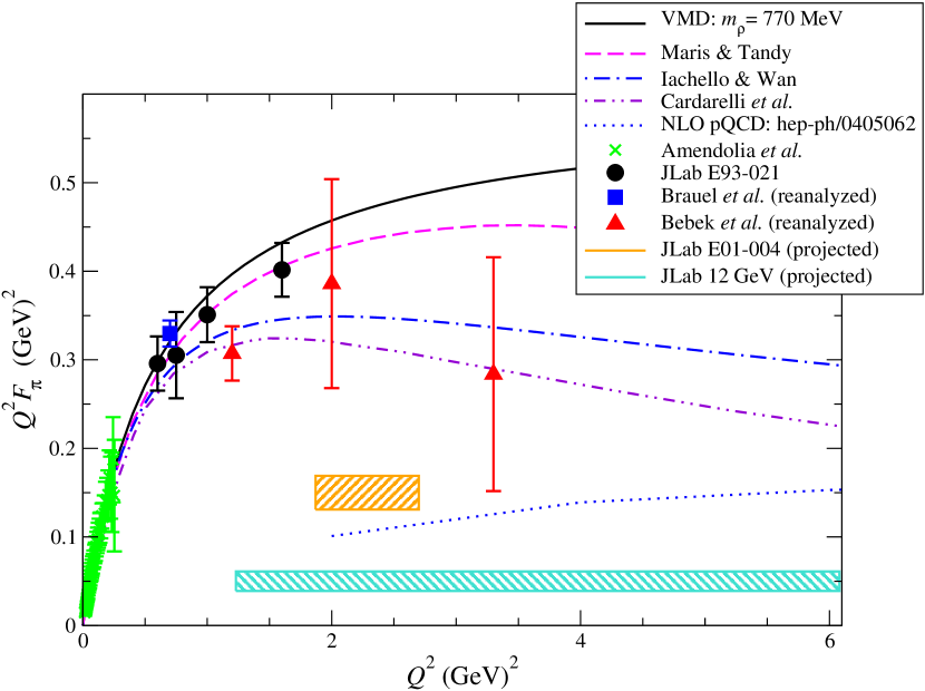
Figure 1: Summary of experimental data for the pion electromagnetic form factor; shaded regions indicate expected sensitivities and coverage of future results. The lines indicate theoretical calculations of the form factor, as described in the text.

For $Q^{2}\leq 0.28\ \mathrm{GeV}^{2}$, Amendolia et al. Amendolia et al. (1986) have determined the form factor to high precision from scattering of very high energy pions from atomic electrons in a fixed target. For higher $Q^{2}$, the form factor has been determined from quasi-elastic scattering from a virtual pion in the proton Bebek et al. (1978); Brauel et al. (1979); Volmer et al. (2001). In this case, the extracted values for the form factor must depend upon some theoretical model Gutbrod and Kramer (1972); Guidal et al. (1997); Vanderhaeghen et al. (1998) for extrapolating the observed scattering from virtual pions to the expected scattering from on-shell pions. As the models have become more sophisticated, the earlier data Bebek et al. (1978); Brauel et al. (1979) have been reanalyzed Blok et al. (2002) for consistency. Shown in Fig. 1 are the results of some model calculations which seem to cover the range of existing predictions Maris and Tandy (2000); Cardarelli et al. (1995); Iachello (2004); Iachello and Wan (2004).

Given the dominance of the rho meson resonance in the time-like region $(Q^{2}<0)$ of the pion form factor, perhaps it is not too surprising that the space-like form factor is well described at low $Q^{2}>0$ by a VMD-inspired monopole form with only a contribution from the lightest vector resonance ($m_{\mathrm{VMD}}\sim m_{\rho}\approx 0.77\ \mathrm{GeV}$). What is striking is that it accurately describes all experimental data even up to scales of $Q^{2}\gtrsim 1\ \mathrm{GeV}^{2}$. Furthermore, VMD predicts that the form factor should scale as $F_{\pi}(Q^{2})\sim 1/Q^{2}$ for $Q^{2}\gg m_{\mathrm{VMD}}^{2}$, the same scaling predicted at asymptotically high $Q^{2}$ in perturbative QCD Brodsky and Farrar (1973, 1975). One crucial fact which makes the pion form factor an ideal observable for studying the interplay between perturbative and non-perturbative QCD is that its asymptotic normalization can be determined from pion decayRadyushkin (1977); Efremov and Radyushkin (1979); Efremov and Radyushkin (1980a, b); Jackson (1977); Farrar and Jackson (1979); Lepage and Brodsky (1979)

$$F_{\pi}(Q^{2})=\frac{8\pi\alpha_{s}(Q^{2})f_{\pi}^{2}}{Q^{2}}\quad\mathrm{as}\quad Q^{2}\to\infty.$$ (2)

Higher order perturbative calculations of the hard contribution to the form factor Stefanis et al. (1999, 1998, 2000); Bakulev et al. (2004) do not vary significantly from this value, and are shown in Fig. 1. At the largest energy scale where reliable experimental measurements have so far been obtained, around $Q^{2}\simeq 2\ \mathrm{GeV}^{2}$, the data are 100% larger than this pQCD asymptotic prediction.

This situation raises many questions. At what scale does the form factor vary with $Q^{2}$ as predicted by pQCD? However, merely observing the proper $Q^{2}$ dependence is insufficient as Eq. (1) has the same asymptotic $Q^{2}$ dependence as pQCD but is numerically about twice as large. How rapidly will the data approach the pQCD prediction and at what scale will pQCD finally agree with the data? These are questions which Lattice QCD calculations are ideally suited to address, provided we can get reliable results for momentum transfer on the order of a few to several $\mathrm{GeV}^{2}$.

Early lattice calculations validated the vector meson dominance hypothesis at low $Q^{2}$ Martinelli and Sachrajda (1988); Draper et al. (1989). Recent lattice results van der Heide et al. (2003); van der Heide et al. (2004a, b); Nemoto (2004); Abdel-Rehim and Lewis (2004a, b), including some of our own preliminary results Bonnet et al. (2004a, b), have somewhat extended the range of momentum transfer, up to $2\ \mathrm{GeV}^{2}$, and the results remain consistent with VMD and the experimental data.

II LATTICE COMPUTATION OF $F_{\pi}(Q^{2})$

The electromagnetic form factor is obtained in lattice QCD simulations by placing a charged pion creation operator at Euclidean time $t_{i}$, a charged pion annihilation operator at $t_{f}$ and a vector current insertion at $t$ as shown in Fig. 2. A standard quark propagator calculation provides the two propagator lines that originate from $t_{i}$. The remaining quark propagator, originating from $t_{f}$ is obtained via the sequential source method: (1) completely specify the quantum numbers, including momentum $\mbox{\boldmath$\mathrm{p}$}_{f}$, of the annihilation operator to be placed at $t_{f}$ and (2) contract the propagator from $t_{i}$ to $t_{f}$ to the annihilation operator and use that product as the source vector of a second, sequential propagator inversion. The resulting sequential propagator appears as the thick line in Fig. 2 extending from $t_{i}$ to $t$ via $t_{f}$. Given these two propagators, the diagram can be computed for all possible values of insertion position $t$ and insertion momenta $\mathrm{q}$; the initial momentum $\mbox{\boldmath$\mathrm{p}$}_{i}$ is determined by momentum conservation $\mbox{\boldmath$\mathrm{p}$}_{i}=\mbox{\boldmath$\mathrm{p}$}_{f}-\mbox{\boldmath$\mathrm{q}$}$.

Furthermore, with the same set of propagators, any current can be inserted at $t$ and any meson creation operator can be contracted at $t_{i}$. So, the diagram relevant to determining the form factor for the transition $\rho^{+}\to\gamma^{*}\pi^{+}$ can be computed without further quark propagator calculations. By applying the sequential source method at the sink, the trade-off is that the entire set of sequential propagators must be recomputed each time new quantum numbers are needed at the sink, particularly $\mbox{\boldmath$\mathrm{p}$}_{f}$.

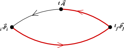
Figure 2: The quark propagators used to compute the pion form factor.

We can extract the pion energies $E_{\pi}(\mbox{\boldmath$\mathrm{p}$})$ using standard lattice techniques of fitting pion correlation functions from which we can compute the momentum transfer

$$-Q^{2}=\left[E_{\pi}(\mbox{\boldmath$\mathrm{p}$}_{f})-E_{\pi}(\mbox{\boldmath$\mathrm{p}$}_{i})\right]^{2}-(\mbox{\boldmath$\mathrm{p}$}_{f}-\mbox{\boldmath$\mathrm{p}$}_{i})^{2}$$ (3)

which should be non-positive if the pion spectral function is well-behaved. Since the largest $Q^{2}$ for a given $\left|\mbox{\boldmath$\mathrm{p}$}\right|^{2}$ occurs in the Breit frame, $\mbox{\boldmath$\mathrm{p}$}_{f}=-\mbox{\boldmath$\mathrm{p}$}_{i}$, it is important to choose a non-zero $\mbox{\boldmath$\mathrm{p}$}_{f}$ to achieve large momentum transfer; indeed $\mbox{\boldmath$\mathrm{p}$}_{f}=\mbox{\boldmath$\mathrm{0}$}$ yields a vanishing $Q^{2}$ for all $\mathrm{q}$ in the chiral limit.

The form factor, $F(Q^{2})$, is defined by

$$\left\langle\pi(\mbox{\boldmath$\mathrm{p}$}_{f})\left|V_{\mu}(0)\right|\pi(\mbox{\boldmath$\mathrm{p}$}_{i})\right\rangle_{\mathrm{continuum}}=Z_{V}\left\langle\pi(\mbox{\boldmath$\mathrm{p}$}_{f})\left|V^{\mathrm{lat}}_{\mu}(0)\right|\pi(\mbox{\boldmath$\mathrm{p}$}_{i})\right\rangle=F(Q^{2})(p_{i}+p_{f})_{\mu}$$ (4)

where $V^{\mathrm{lat}}_{\mu}(x)$ is a particular lattice discretization of the continuum vector current. In this work, local and point-split vector currents were used:

$$V_{\mu}^{\mathrm{loc}}(x) = \overline{\psi}(x)\gamma_{\mu}\psi(x)$$ (5)

$$V_{\mu}^{\mathrm{p.s.}}(x) = \frac{1}{2}\left\{\overline{\psi}(x+\widehat{\mu})U_{\mu}^{\dagger}(x)\left[1+\gamma_{\mu}\right]\psi(x)-\overline{\psi}(x)U_{\mu}(x)\left[1-\gamma_{\mu}\right]\psi(x+\widehat{\mu})\right\}.$$ (6)

$Z_{V}$ is the corresponding matching factor between the lattice current and continuum; for Wilson fermions, the point-split current is conserved on the lattice: $Z_{V}^{\mathrm{p.s.}}=1$ (Wilson). The three-point correlation function depicted in Fig. 2 is given by

$$\Gamma_{\pi\mu\pi}^{AB}(t_{i},t,t_{f},\mbox{\boldmath$\mathrm{p}$}_{i},\mbox{\boldmath$\mathrm{p}$}_{f})=\sum_{\mbox{\boldmath$\mathrm{x}$}_{i},\mbox{\boldmath$\mathrm{x}$}_{f}}e^{-i(\mbox{\boldmath$\mathrm{x}$}_{f}-\mbox{\boldmath$\mathrm{x}$})\cdot\mbox{\boldmath$\mathrm{p}$}_{f}}\ e^{-i(\mbox{\boldmath$\mathrm{x}$}-\mbox{\boldmath$\mathrm{x}$}_{i})\cdot\mbox{\boldmath$\mathrm{p}$}_{i}}\left\langle 0\left|\phi_{B}(x_{f})V_{\mu}(x)\phi_{A}^{\dagger}(x_{i})\right|0\right\rangle$$ (7)

where $\phi_{A}^{\dagger}(x)$ and $\phi_{B}(x)$ are creation and annihilation operators with pion quantum numbers. The $A$ and $B$ indicate that different operators may be used at the source and sink, i.e. smeared source and point sink or pseudoscalar source and axial vector sink.

Inserting complete sets of hadron states, and requiring $t_{i}\ll t\ll t_{f}$, gives

$$\Gamma_{\pi\mu\pi}^{AB}(t_{i},t,t_{f},\mbox{\boldmath$\mathrm{p}$}_{i},\mbox{\boldmath$\mathrm{p}$}_{f})\to\left\langle 0\left|\phi_{B}(0)\right|\pi(\mbox{\boldmath$\mathrm{p}$}_{f})\right\rangle\frac{e^{-(t_{f}-t)E_{\pi}(\mbox{\boldmath$\mathrm{p}$}_{f})}}{2E_{\pi}(\mbox{\boldmath$\mathrm{p}$}_{f})}\left\langle\pi(\mbox{\boldmath$\mathrm{p}$}_{f})\left|V_{\mu}(0)\right|\pi(\mbox{\boldmath$\mathrm{p}$}_{i})\right\rangle\frac{e^{-(t-t_{i})E_{\pi}(\mbox{\boldmath$\mathrm{p}$}_{i})}}{2E_{\pi}(\mbox{\boldmath$\mathrm{p}$}_{i})}\left\langle\pi(\mbox{\boldmath$\mathrm{p}$}_{i})\left|\phi_{A}^{\dagger}(0)\right|0\right\rangle.$$ (8)

Similarly for the two-point correlator, with $t_{i}\ll t_{f}$,

$$\Gamma_{\pi\pi}^{AB}(t_{i},t_{f},\mbox{\boldmath$\mathrm{p}$})\to\left\langle 0\left|\phi_{B}(0)\right|\pi(\mbox{\boldmath$\mathrm{p}$})\right\rangle\frac{e^{-(t_{f}-t_{i})E_{\pi}(\mbox{\boldmath$\mathrm{p}$})}}{2E_{\pi}(\mbox{\boldmath$\mathrm{p}$})}\left\langle\pi(\mbox{\boldmath$\mathrm{p}$})\left|\phi_{A}^{\dagger}(0)\right|0\right\rangle.$$ (9)

We use both the pseudoscalar density, $\phi^{(1)}(x)=\overline{\psi}(x)\gamma_{5}\psi(x)$, and the temporal component of the axial vector current, $\phi^{(2)}(x)=\overline{\psi}(x)\gamma_{5}\gamma_{4}\psi(x)$, as pion interpolating operators, constructed from both local and smeared quark fields, denoted by L and S respectively. We adopt gauge-invariant Gaussian smearing

$$b(x)\to\left(1+\frac{\omega}{N}\mbox{\boldmath$\mathrm{\nabla}$}U\right)^{N}b(x),$$ (10)

where $\omega$ and $N$ are the tunable parameters used to specify the smearing radius; the flavor structure is suppressed. The respective merits of these interpolating operators will be discussed later. For these operators, we define the following amplitudes

$$\left\langle 0\left|\phi_{L}^{(1)}(0)\right|\pi(\mbox{\boldmath$\mathrm{p}$})\right\rangle = Z_{L}^{(1)}$$ (11)

$$\left\langle 0\left|\phi_{S}^{(1)}(0)\right|\pi(\mbox{\boldmath$\mathrm{p}$})\right\rangle = Z_{S}^{(1)}(\left|\mbox{\boldmath$\mathrm{p}$}\right|)$$ (12)

$$\left\langle 0\left|\phi_{L}^{(2)}(0)\right|\pi(\mbox{\boldmath$\mathrm{p}$})\right\rangle = Z_{L}^{(2)}(\left|\mbox{\boldmath$\mathrm{p}$}\right|)$$ (13)

$$\left\langle 0\left|\phi_{S}^{(2)}(0)\right|\pi(\mbox{\boldmath$\mathrm{p}$})\right\rangle = Z_{S}^{(2)}(\left|\mbox{\boldmath$\mathrm{p}$}\right|).$$ (14)

The overlap of the operator $\phi_{L}^{(2)}$ has trivial $\mathrm{p}$ dependence arising from the Lorentz structure of the operator

$$Z_{L}^{(2)}=E(\mid\mbox{\boldmath$\mathrm{p}$}\mid)f_{\pi}.$$ (15)

However, the introduction of an additional three-dimensional scale introduces non-trivial $\mathrm{p}$ dependence for the smeared overlaps $Z_{S}^{(1)}$ and $Z_{S}^{(2)}$.

We employ two methods to determine the form factor $F_{\pi}(Q^{2})$. The first method, which we call the fitting method, involves a fit of the relevant two- and three-point functions to simultaneously extract the form factor, the energies $E_{\pi}(\mbox{\boldmath$\mathrm{p}$})$ and the amplitudes $Z(\mbox{\boldmath$\mathrm{p}$})$ in a single covariant, jackknifed fit.

The second method, which we call the ratio method, starts by determining the energies $E_{\pi}(\mbox{\boldmath$\mathrm{p}$})$, either by fits to the correlators at non-zero momentum or from a dispersion relation, and then constructing the following ratio which is independent of $Z_{L}^{(1)}$, $Z_{S}(|\mbox{\boldmath$\mathrm{p}$}|)$ and all Euclidean time exponentials for sufficiently large temporal separations:

$$F(Q^{2},t)=\frac{\Gamma_{\pi 4\pi}^{AB}(t_{i},t,t_{f},\mbox{\boldmath$\mathrm{p}$}_{i},\mbox{\boldmath$\mathrm{p}$}_{f})\Gamma_{\pi\pi}^{CL}(t_{i},t,\mbox{\boldmath$\mathrm{p}$}_{f})}{\Gamma_{\pi\pi}^{AL}(t_{i},t,\mbox{\boldmath$\mathrm{p}$}_{i})\Gamma_{\pi\pi}^{CB}(t_{i},t_{f},\mbox{\boldmath$\mathrm{p}$}_{f})}\left(\frac{2Z_{V}E_{\pi}(\mbox{\boldmath$\mathrm{p}$}_{f})}{E_{\pi}(\mbox{\boldmath$\mathrm{p}$}_{i})+E_{\pi}(\mbox{\boldmath$\mathrm{p}$}_{f})}\right)$$ (16)

where the indices $A$, $B$ and $C$ can be either $L$ (local) or $S$ (smeared). As part of our program, we expect to determine the relative merits of each extraction method.

III SIMULATION DETAILS

Our first calculations were performed on quenched configurations generated with the Wilson gauge action at $\beta=6.0$, corresponding to $a^{-1}\approx 2\ \mathrm{GeV}$. The propagators were computed using the unimproved Wilson fermion action with Dirichlet boundary conditions in the temporal direction, and periodic boundary conditions in the spatial directions. For Wilson fermions at these lattice spacings, the exceptional configuration problem is rather mild particularly when compared to that for the non-perturbatively improved clover action. This enabled us to reach pion masses of $300\ \mathrm{MeV}$ without observing any exceptional configurations, whereas computations using the clover action are limited to pion masses in excess of roughly $400\ \mathrm{MeV}$ van der Heide et al. (2003) due to the systematic errors caused by the frequent occurrence of exceptional configurations. A detailed listing of the simulation parameters is provided in Tab. 1.

Table 1: Simulation details for quenched Wilson fermion calculations at $a^{-1}\approx 2\ \mathrm{GeV}$

. $\kappa$ volume $am_{\rho}$ $am_{\pi}$ $m_{\pi}/m_{\rho}$ $m_{\pi}L$ $Z_{V}^{\mathrm{loc}}$ 0.1480 $16^{3}\times 32$ 0.7187(39) 0.6752(45) 0.943(10) 10.80(7) 0.82725(51) 0.1500 $16^{3}\times 32$ 0.6387(57) 0.5854(45) 0.900(13) 9.36(7) 0.78486(46) 0.1520 $16^{3}\times 32$ 0.5540(83) 0.4851(67) 0.876(14) 7.76(11) 0.74197(54) 0.1540 $16^{3}\times 32$ 0.4682(124) 0.3752(73) 0.801(23) 6.00(11) 0.70459(39) 0.1555 $24^{3}\times 32$ 0.4209(88) 0.2613(29) 0.621(14) 6.27(7) 0.1563 $24^{3}\times 32$ 0.4014(68) 0.1921(29) 0.479(10) 4.61(7) 0.65676(43) 0.1566 $32^{3}\times 48$ 0.3724(145) 0.1629(36) 0.437(19) 5.21(12) 0.65553(14)

The pion masses attainable in quenched domain-wall fermion (DWF) calculations are limited only by finite volume effects and available computing power. So far, however, quenched DWF computations of the pion form factor have only explored pion masses down to $390\ \mathrm{MeV}$, at $a^{-1}\approx 1.3\ \mathrm{GeV}$ Nemoto (2004). An important advantage of DWF fermions is that they are automatically $\mathcal{O}(a)$-improved. An alternative approach using twisted-mass QCD (tmQCD), in which Wilson fermion results are also $\mathcal{O}(a)$ improved with just double the effortFrezzotti and Rossi (2004), has been explored separatelyAbdel-Rehim and Lewis (2004a).

Table 2: Simulation details for domain wall fermion calculations on 20${}^{3}\times$64 dynamical MILC asqtad lattices at $a^{-1}\approx 1.6\ \mathrm{GeV}$.

$am_{ud}$	$am_{s}$	$am_{\mathrm{val}}$	$m_{\rho}\ \mathrm{(MeV)}$	$m_{\pi}\ \mathrm{(MeV)}$	$m_{\pi}/m_{\rho}$	$m_{\pi}L$	$Z_{V}^{\mathrm{loc}}$	$Z_{V}^{\mathrm{p.s.}}$
0.01	0.05	0.01	956(22)	318(3)	0.333(8)	3.97(4)	1.0714(55)	1.1098(23)
0.05	0.05	0.05	955(19)	602(5)	0.630(12)	7.68(6)	1.0890(55)	1.0835(37)
0.05	0.05	0.081	1060(14)	758(5)	0.715(10)	9.66(6)	1.1199(14)	1.0833(13)

The Lattice Hadron Physics Collaboration (LHPC) has been performing unquenched hadron structure calculations using MILC $N_{f}=2+1$ and $N_{f}=3$ configurations generated with staggered asqtad sea quarks Negele et al. (2004b); Schroers et al. (2004); Negele et al. (2004a); Renner et al. (2004); Hägler et al. (2004). Valence propagators were computed using domain wall quarks with domain wall height $m=1.7$ and extent $L_{s}=16$ of the extra dimension and Dirichlet boundary conditions imposed 32 timeslices apart. The MILC configurations were HYP blocked Hasenfratz and Knechtli (2001) before the valence propagators were computed to avoid unacceptably large residual chiral symmetry breaking. For our pion form factor calculation we chose configurations separated by at least 12 HMD trajectories. In some of the other LHPC calculations, if measurements were computed on configurations separated by 6 HMD trajectories, opposite halves of the lattice were used to minimize autocorrelations. The simulation parameters for the DWF computation are provided in Tab. 2. A detailed study of the physical properties of light hadrons composed of staggered quarks computed on these lattices has recently been completed Aubin et al. (2004).

IV RESULTS

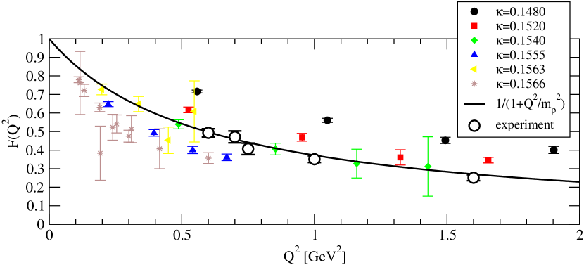
Figure 3: Results for the pion form factor as a function of $Q^{2}$ for each of the available $\kappa$ values, together with experimental determinationsVolmer et al. (2001). The curve shows the vector-meson-dominance prediction, using the experimental determination of the $\rho$ mass.

Results for the quenched Wilson form factor computed by the fitting method at each value of the quark mass are shown in Fig. 3. Also indicated are experimental data points and the vector meson dominance (VMD) prediction using the experimental value for the $\rho$ meson mass. While the data tend in the correct direction with decreasing pion mass, the reader may notice that the form factor for $300\ \mathrm{MeV}$ pions already lies below the physical curve. This suggests that the pole mass that would be obtained from a VMD fit to the lattice data would be considerably lower than the physical $\rho$ meson mass. This is perhaps expected since it is known that $\mathcal{O}(a)$ scaling violations in the vector meson mass computed with Wilson fermions yield an underestimate of the mass of roughly 20% Edwards et al. (1998), the same amount needed to move the form factor points so as to lie above the continuum curve.

Because we would like to compute the pion form factor at large momentum transfer, we have spent a substantial amount of effort on our domain wall data set in extracting the pion energies and amplitudes at relatively large momenta; the largest attainable momenta is constrained by the fineness of the lattice spacing. In the continuum limit, the pion dispersion relation should approach the continuum one

$$E_{\pi}(\mbox{\boldmath$\mathrm{p}$})^{2}=\mbox{\boldmath$\mathrm{p}$}^{2}+E_{\pi}(0)^{2}.$$ (17)

At a non-zero lattice spacing, a study of free lattice bosons suggests the lattice dispersion relation

$$\widehat{E}(\mbox{\boldmath$\mathrm{\widehat{p}}$})^{2}=\mbox{\boldmath$\mathrm{\widehat{p}}$}^{2}+\widehat{E}_{\pi}(0)^{2}$$ (18)

where $\widehat{E}$ and $\widehat{p}$ are the “lattice” energy and momentum respectively:

$$\widehat{E}=2\sinh\left(\frac{E}{2}\right)\qquad\widehat{p}_{x}=2\sin\left(\frac{p_{x}}{2}\right).$$ (19)

Eqs. (17) and (18) agree in the small-momentum limit.

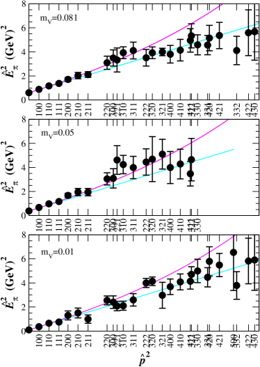
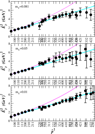
Figure 4: Pion (left) and rho meson (right) dispersion relation vs. continuum (upper) and lattice (lower) expectations curves.

In Fig. 4, we show the measured “lattice” energies against the lattice momenta at each of our quark masses, together with curves representing the continuum and lattice dispersion relations. We see that both dispersion relations provide a reasonable representation of the data, although there may be a slight flattening of the data against the continuum curve at higher momenta. These results suggest that directly fitting all the data to either dispersion relation, thereby reducing the number of fit parameters needed to extract the form factor, may improve the relative signal to noise of the remaining parameters. This may help dramatically in the ratio method, where the only fit parameters are the form factor and the energies.

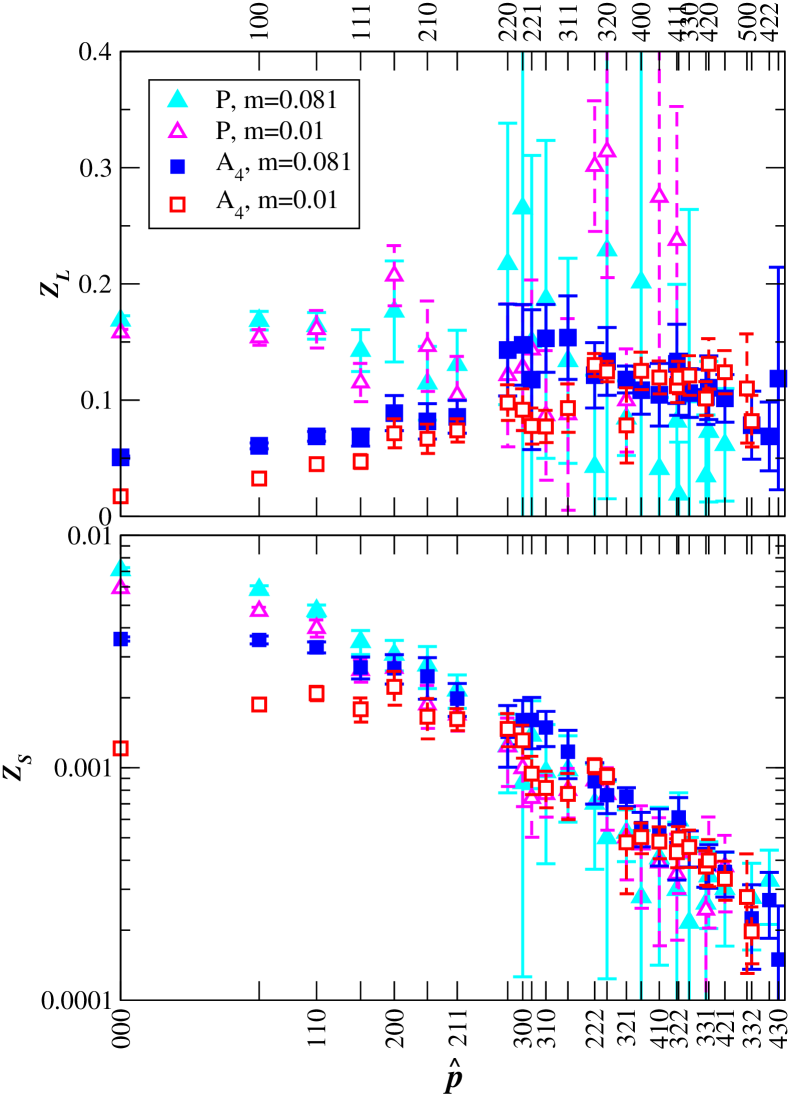
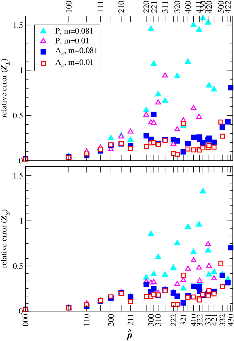
Figure 5: Results for the local (L) and smeared (S) pseudoscalar ( $\blacktriangle$, $\vartriangle$) and axial vector ( $\blacksquare$, $\square$) pion source amplitudes $Z_{A}^{(i)}(\mbox{\boldmath$\mathrm{p}$})$ used in this study.

In the fitting method, one must reliably extract not only the energies, but the amplitudes, at high momenta. In Fig. 5 we present the four amplitudes of Eqs. (11) through (14) that we estimate from the four two-point correlators we measure: smeared-smeared and smeared-local for both pseudoscalar-pseudoscalar and axial-axial operators. In the fitting procedure, all four correlators are constrained to have the same energy. From the figure, we can see that our expectations of $Z_{L}^{(1)}\propto\mathit{const}$ and $Z_{L}^{(2)}(\mbox{\boldmath$\mathrm{p}$})\propto E_{\pi}(\mbox{\boldmath$\mathrm{p}$})$ are consistent with the data. We can also see from $Z_{S}^{(1)}(\mbox{\boldmath$\mathrm{p}$}=0)$ that the smeared pseudoscalar operator has a strong overlap with the zero momentum pion relative to the axial-vector operator.

We plot in Fig. 5 just the relative error estimates for the amplitudes. This clearly demonstrates that the statistical noise inherent in a particular source or sink operator need not be correlated with the magnitude of the amplitude. In particular, we see that beyond the few smallest momenta, the pseudoscalar and axial-vector amplitudes are of the same order, but the inherent noise of the pseudoscalar operator is unacceptably large for higher momenta.

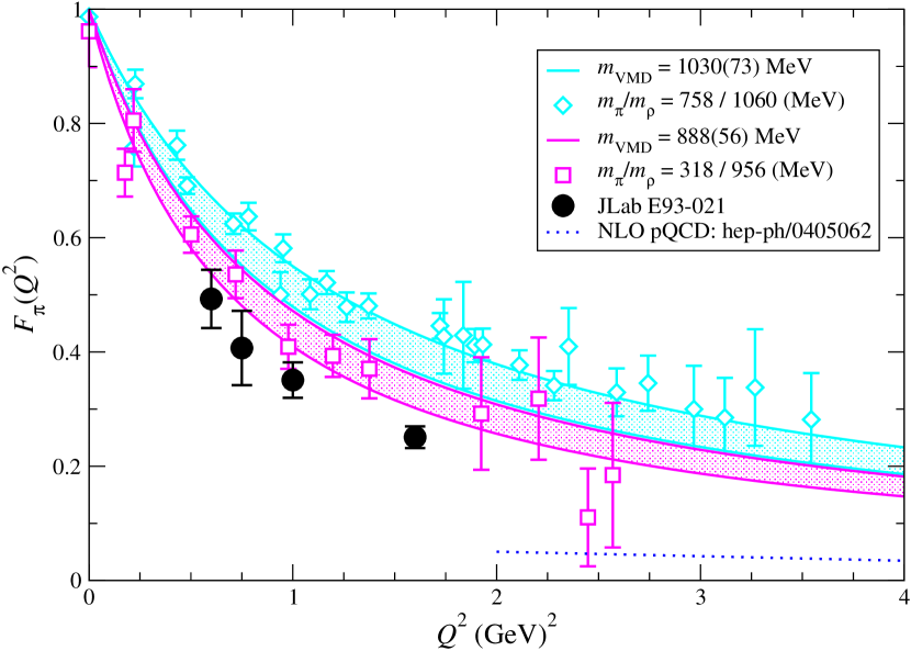
Figure 6: Pion electromagnetic form factor for fixed sink momentum $\mbox{\boldmath$\mathrm{p}$}_{f}=(1,0,0)$ computed by the ratio method Bonnet et al. (2004a, b) and imposing the lattice dispersion relation, Eq. (18). Shaded regions are jackknife error bands for VMD fit.

Table 3: Results of fit of form factor data to the VMD monopole ansatz of Eq. (1).

$am_{\mathrm{val}}$	$\mbox{\boldmath$\mathrm{p}$}_{f}$	$m_{\mathrm{VMD}}$ (GeV)	$\chi^{2}/\mathrm{d.o.f.}$	$\mathrm{d.o.f.}$	$N_{\mathrm{confs}}$
0.01	(0,0,0)	—	—	—	51
	(1,0,0)	0.888(56)	1.37(72)	13	251
	(1,1,0)	0.30(20)	1.7(1.2)	11	106
0.05	(0,0,0)	1.278(87)	2.8(1.3)	20	104
0.081	(0,0,0)	1.192(93)	3(17)	15	49
	(1,0,0)	1.030(73)	2.1(1.7)	22	70
	(1,1,0)	1.022(87)	3.6(2.2)	23	73

Using the lattice dispersion relation and the ratio method described above and in our previous work, we have computed in Fig. 6 the pion form factor for two of the dynamical pion masses. Fits of the data to the monopole form of Eq. (1) are also shown, where shaded regions correspond to jackknife error bands and the central values for the pole masses are given in the legend. The data in Fig. 6 were computed with pseudoscalar pion sink operator fixed at momentum $\mbox{\boldmath$\mathrm{p}$}_{f}=(1,0,0)$. Tab. 3 summarizes the fits for all available combinations of $m_{\mathrm{val}}$ and $\mbox{\boldmath$\mathrm{p}$}_{f}$. Unconstrained linear extrapolation of the two most reliable data points, $m_{\mathrm{val}}=0.01$ and 0.081 with $\mbox{\boldmath$\mathrm{p}$}_{f}=(1,1,0)$, gives an estimate of $m_{\mathrm{VMD}}=0.868(65)\ \mathrm{GeV}$ in the zero quark mass limit. From this we estimate the mean square charge radius of the pion to be $\left\langle r^{2}\right\rangle_{\mathrm{VMD}}=0.310(46)\ \mathrm{fm}^{2}$, which is significantly below the experimental value of $\left\langle r^{2}\right\rangle_{\mathrm{expt}}=0.439(8)\ \mathrm{fm}^{2}$. More dynamical quark masses, particularly lighter ones, will be needed to perform a proper chiral extrapolation.

We were unable to compute statistically significant form factors with the same pseudoscalar sink operator for $m_{\mathrm{val}}=0.01$ and $\mbox{\boldmath$\mathrm{p}$}_{f}=(1,1,0)$ by the ratio method, apparently due to the poor signal-to-noise inherent in the overlap of the chosen sink operator with the higher momentum state. For $m_{\mathrm{val}}=0.01$ and $\mbox{\boldmath$\mathrm{p}$}_{f}=(0,0,0)$ the signal was rather better but 51 sequential propagators were too few to allow for a stable fit to the VMD ansatz. We expect that an axial vector sink operator would be a better choice for future calculations at non-zero sink momentum. Some of us are also extending our group-theoretical construction of extended baryon operators Edwards et al. (2004); Basak et al. (2004a, b, c, d) to include mesonic quantum numbers.

V CONCLUSIONS

From our quenched Wilson form factor results, we find that both the ratio method and the fitting method are useful tools for computing the pion form factor. Each method has different systematic errors, so the extent to which both agree should give confidence that the systematic errors are small and well understood. A comparison of the Wilson form factor results with the experimental pion form factor data suggests that the former have large, and expected, discretization errors.

Domain-wall fermions are free of ${\cal O}(a)$ discretization uncertainties to the extent that any residual mass is eliminated. Thus our dynamical fermion results are obtained using domain-wall fermions for the valence quarks computed on asqtad lattices. From a careful analysis of the pion spectrum, we recognize the importance of using a large basis of pion operators so that we can identify at least one operator at each pion momentum whose overlap with the pion has a reasonable signal-to-noise ratio. The local axial vector operator appears to be a better choice than the pseudoscalar operator for fitting higher momentum states since its overlap with a given state increases in proportion with the pion energy and without any degradation of the signal-to-noise ratio. Our analysis enables us to obtain the pion form factor for a pion mass approaching $300~{}{\rm MeV}$ at a range of $Q^{2}$ commensurate with the current experimental program.

Given our existing analysis framework and the propagators and sequential propagators that we have already computed, we can also compute the $\rho^{+}\to\gamma\pi^{+}$ transition form factor. We hope to complete this analysis in the near future.

References

- Isgur and Llewellyn Smith (1984) N. Isgur and C. H. Llewellyn Smith, Phys. Rev. Lett. 52, 1080 (1984).
- Holladay (1956) W. G. Holladay, Phys. Rev. 101, 1198 (1956).
- Frazer and Fulco (1959) W. R. Frazer and J. R. Fulco, Phys. Rev. Lett. 2, 365 (1959).
- Frazer and Fulco (1960) W. R. Frazer and J. R. Fulco, Phys. Rev. 117, 1609 (1960).
- Amendolia et al. (1986) S. R. Amendolia et al. (NA7), Nucl. Phys. B277, 168 (1986).
- Bebek et al. (1978) C. J. Bebek et al., Phys. Rev. D17, 1693 (1978).
- Brauel et al. (1979) P. Brauel et al., Zeit. Phys. C3, 101 (1979).
- Volmer et al. (2001) J. Volmer et al. (The Jefferson Lab F(pi)), Phys. Rev. Lett. 86, 1713 (2001), eprint nucl-ex/0010009.
- Gutbrod and Kramer (1972) F. Gutbrod and G. Kramer, Nucl. Phys. B49, 461 (1972).
- Guidal et al. (1997) M. Guidal, J. M. Laget, and M. Vanderhaeghen, Nucl. Phys. A627, 645 (1997).
- Vanderhaeghen et al. (1998) M. Vanderhaeghen, M. Guidal, and J. M. Laget, Phys. Rev. C57, 1454 (1998).
- Blok et al. (2002) H. P. Blok, G. M. Huber, and D. J. Mack (2002), eprint nucl-ex/0208011.
- Maris and Tandy (2000) P. Maris and P. C. Tandy, Phys. Rev. C62, 055204 (2000), eprint nucl-th/0005015.
- Cardarelli et al. (1995) F. Cardarelli, E. Pace, G. Salme, and S. Simula, Phys. Lett. B357, 267 (1995), eprint nucl-th/9507037.
- Iachello (2004) F. Iachello, Eur. Phys. J. A19, Suppl129 (2004).
- Iachello and Wan (2004) F. Iachello and Q. Wan (2004), in preparation.
- Brodsky and Farrar (1973) S. J. Brodsky and G. R. Farrar, Phys. Rev. Lett. 31, 1153 (1973).
- Brodsky and Farrar (1975) S. J. Brodsky and G. R. Farrar, Phys. Rev. D11, 1309 (1975).
- Farrar and Jackson (1979) G. R. Farrar and D. R. Jackson, Phys. Rev. Lett. 43, 246 (1979).
- Radyushkin (1977) A. V. Radyushkin (1977), eprint hep-ph/0410276.
- Efremov and Radyushkin (1979) A. V. Efremov and A. V. Radyushkin, in Proceedings of the XIX International Conference on High Energy Physics, Tokyo, Japan, August 23-30, 1978, edited by S. Homma (Physical Society of Japan, Tokyo, 1979), jINR-E2-11535.
- Efremov and Radyushkin (1980a) A. V. Efremov and A. V. Radyushkin, Theor. Math. Phys. 42, 97 (1980a).
- Efremov and Radyushkin (1980b) A. V. Efremov and A. V. Radyushkin, Phys. Lett. B94, 245 (1980b).
- Jackson (1977) D. R. Jackson, Ph.D. thesis, California Institute of Technology (1977).
- Lepage and Brodsky (1979) G. P. Lepage and S. J. Brodsky, Phys. Lett. B87, 359 (1979).
- Stefanis et al. (1999) N. G. Stefanis, W. Schroers, and H.-C. Kim, Phys. Lett. B449, 299 (1999), eprint hep-ph/9807298.
- Stefanis et al. (1998) N. G. Stefanis, W. Schroers, and H.-C. Kim (1998), eprint hep-ph/9812280.
- Stefanis et al. (2000) N. G. Stefanis, W. Schroers, and H.-C. Kim, Eur. Phys. J. C18, 137 (2000), eprint hep-ph/0005218.
- Bakulev et al. (2004) A. P. Bakulev, K. Passek-Kumericki, W. Schroers, and N. G. Stefanis (2004), eprint hep-ph/0405062.
- Martinelli and Sachrajda (1988) G. Martinelli and C. T. Sachrajda, Nucl. Phys. B306, 865 (1988).
- Draper et al. (1989) T. Draper, R. M. Woloshyn, W. Wilcox, and K.-F. Liu, Nucl. Phys. B318, 319 (1989).
- van der Heide et al. (2003) J. van der Heide, M. Lutterot, J. H. Koch, and E. Laermann, Phys. Lett. B566, 131 (2003), eprint hep-lat/0303006.
- Nemoto (2004) Y. Nemoto (RBC), Nucl. Phys. Proc. Suppl. 129, 299 (2004), eprint hep-lat/0309173.
- Abdel-Rehim and Lewis (2004a) A. M. Abdel-Rehim and R. Lewis (2004a), eprint hep-lat/0408033.
- Abdel-Rehim and Lewis (2004b) A. M. Abdel-Rehim and R. Lewis (2004b), eprint hep-lat/0410047.
- van der Heide et al. (2004a) J. van der Heide, J. H. Koch, and E. Laermann, Phys. Rev. D69, 094511 (2004a), eprint hep-lat/0312023.
- van der Heide et al. (2004b) J. van der Heide, J. H. Koch, and E. Laermann (2004b), eprint hep-lat/0410006.
- Bonnet et al. (2004a) F. D. R. Bonnet, R. G. Edwards, G. T. Fleming, R. Lewis, and D. G. Richards, Nucl. Phys. Proc. Suppl. 129, 206 (2004a), eprint hep-lat/0310053.
- Bonnet et al. (2004b) F. D. R. Bonnet, R. G. Edwards, G. T. Fleming, R. Lewis, and D. G. Richards (LHP), Nucl. Phys. Proc. Suppl. 128, 59 (2004b), eprint hep-lat/0312008.
- Frezzotti and Rossi (2004) R. Frezzotti and G. C. Rossi, Nucl. Phys. Proc. Suppl. 128, 193 (2004), eprint hep-lat/0311008.
- Negele et al. (2004a) J. W. Negele et al. (LHP), Nucl. Phys. Proc. Suppl. 128, 170 (2004a), eprint hep-lat/0404005.
- Renner et al. (2004) D. B. Renner et al. (LHP) (2004), eprint hep-lat/0409130.
- Negele et al. (2004b) J. W. Negele et al. (LHP), Nucl. Phys. Proc. Suppl. 129, 910 (2004b), eprint hep-lat/0309060.
- Schroers et al. (2004) W. Schroers et al. (LHP), Nucl. Phys. Proc. Suppl. 129, 907 (2004), eprint hep-lat/0309065.
- Hägler et al. (2004) P. Hägler et al. (LHP) (2004), eprint hep-ph/0410017.
- Hasenfratz and Knechtli (2001) A. Hasenfratz and F. Knechtli, Phys. Rev. D64, 034504 (2001), eprint hep-lat/0103029.
- Aubin et al. (2004) C. Aubin et al. (MILC) (2004), eprint hep-lat/0402030.
- Edwards et al. (1998) R. G. Edwards, U. M. Heller, and T. R. Klassen, Phys. Rev. Lett. 80, 3448 (1998), eprint hep-lat/9711052.
- Edwards et al. (2004) R. Edwards et al. (LHP), Nucl. Phys. Proc. Suppl. 129, 236 (2004), eprint hep-lat/0309079.
- Basak et al. (2004a) S. Basak et al. (LHP), Nucl. Phys. Proc. Suppl. 129, 209 (2004a), eprint hep-lat/0309091.
- Basak et al. (2004b) S. Basak et al. (LHP), Nucl. Phys. Proc. Suppl. 128, 186 (2004b), eprint hep-lat/0312003.
- Basak et al. (2004c) S. Basak et al. (LHP) (2004c), eprint hep-lat/0409080.
- Basak et al. (2004d) S. Basak et al. (LHP) (2004d), eprint hep-lat/0409093.